Populating Input Spaces: Conceptual Blending and the Historical Thesaurus of English

Presented at the 13th International Cognitive Linguistics Conference

Authors:
Marc Alexander, University of Glasgow
Fraser Dallachy, University of Glasgow

Transcript

1. Populating input spaces M A R C A L E X A N D E R A N D F R A S E R D A L L A C H Y, U N I V E R S I T Y O F G L A S G O W Conceptual Blending and the Historical Thesaurus of English
2. E A S I E R T O U R D E F O R C E S ? ‘When we see the final integration network with all of its connections in place, it may look like a tour de force showing the mastery of its creator in selecting just the right projections […] There is always extensive unconscious work in meaning construction, and blending is no different. We may make many parallel attempts to find suitable projections, with only the accepted ones appearing in the final network. […] Input formation, projection, completion and elaboration all go on at the same time, and a lot of conceptual scaffolding goes up that we never see in the final result. Brains always do a lot of work that gets thrown away.’ Fauconnier and Turner 2002: 71-72
3. H T A N D C L Although the project was started before the current cognitive semantics paradigm became dominant, that paradigm has retrospectively proved sympathetic to the problems involved in categorizing large quantities of lexical data. The development of prototype theory, which allows for fuzzy sets containing both good and less good examples of the central concept, challenges the either/or basis of Aristotelian category assignment and liberates semanticists from a narrow notion of synonymy as an organizing principle. HT’s synonym groupings are prototypical in nature, with a clear core of obvious members shading off into the less obvious, and ultimately into cognate categories. Kay et al 2009: xix
4. Semantic Annotation System VARD CLAWS HT sense tagger USAS NLP lexicon resources USAS [HT-related resources] Historical Thesaurus; Higher-level HT categories; Linked HT categories; Highly polysemous words; Z-category words; Polyseme density list; Input raw text Annotated text HT sense disambiguator Spelling training model
6. O U T L I N E
7. O U T L I N E 1. Identify input spaces.
8. O U T L I N E 1. Identify input spaces. 2. Describe the constitution of the input spaces identified. Use SAMUELS tagging to label input spaces with HT categories.
9. O U T L I N E 1. Identify input spaces. 2. Describe the constitution of the input spaces identified. Use SAMUELS tagging to label input spaces with HT categories. 3. Outline the internal makeup of the input spaces
10. O U T L I N E 1. Identify input spaces. 2. Describe the constitution of the input spaces identified. Use SAMUELS tagging to label input spaces with HT categories. 3. Outline the internal makeup of the input spaces 4. List relationships between the input spaces in the text.
11. O U T L I N E 1. Identify input spaces. 2. Describe the constitution of the input spaces identified. Use SAMUELS tagging to label input spaces with HT categories. 3. Outline the internal makeup of the input spaces 4. List relationships between the input spaces in the text. 5. Detail the vital relations which each relationship identified in stage 4 above instantiates, both first- and second-order.
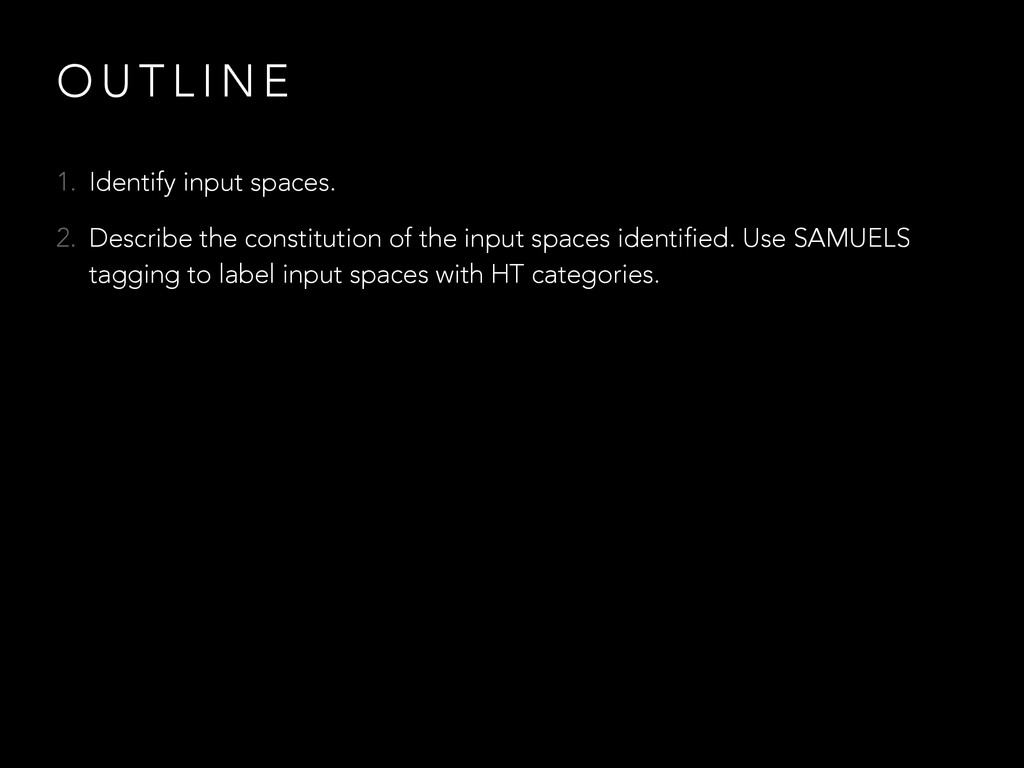
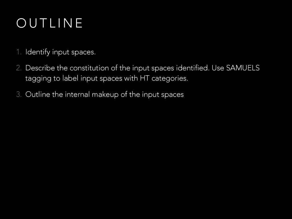
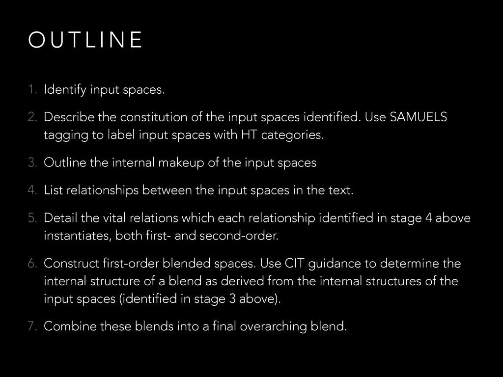
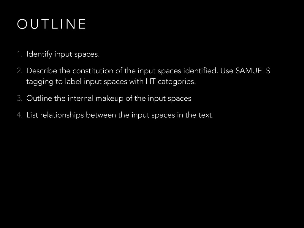
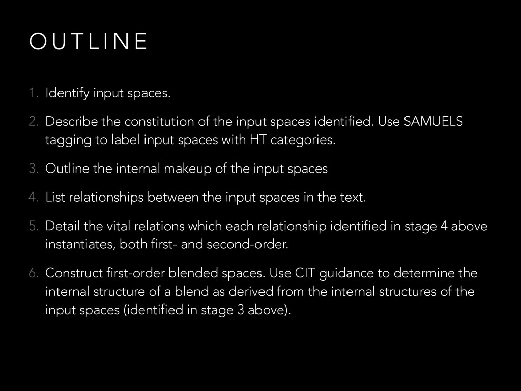
12. O U T L I N E 1. Identify input spaces. 2. Describe the constitution of the input spaces identified. Use SAMUELS tagging to label input spaces with HT categories. 3. Outline the internal makeup of the input spaces 4. List relationships between the input spaces in the text. 5. Detail the vital relations which each relationship identified in stage 4 above instantiates, both first- and second-order. 6. Construct first-order blended spaces. Use CIT guidance to determine the internal structure of a blend as derived from the internal structures of the input spaces (identified in stage 3 above).
13. O U T L I N E 1. Identify input spaces. 2. Describe the constitution of the input spaces identified. Use SAMUELS tagging to label input spaces with HT categories. 3. Outline the internal makeup of the input spaces 4. List relationships between the input spaces in the text. 5. Detail the vital relations which each relationship identified in stage 4 above instantiates, both first- and second-order. 6. Construct first-order blended spaces. Use CIT guidance to determine the internal structure of a blend as derived from the internal structures of the input spaces (identified in stage 3 above). 7. Combine these blends into a final overarching blend.
14. I N P R A C T I C E …
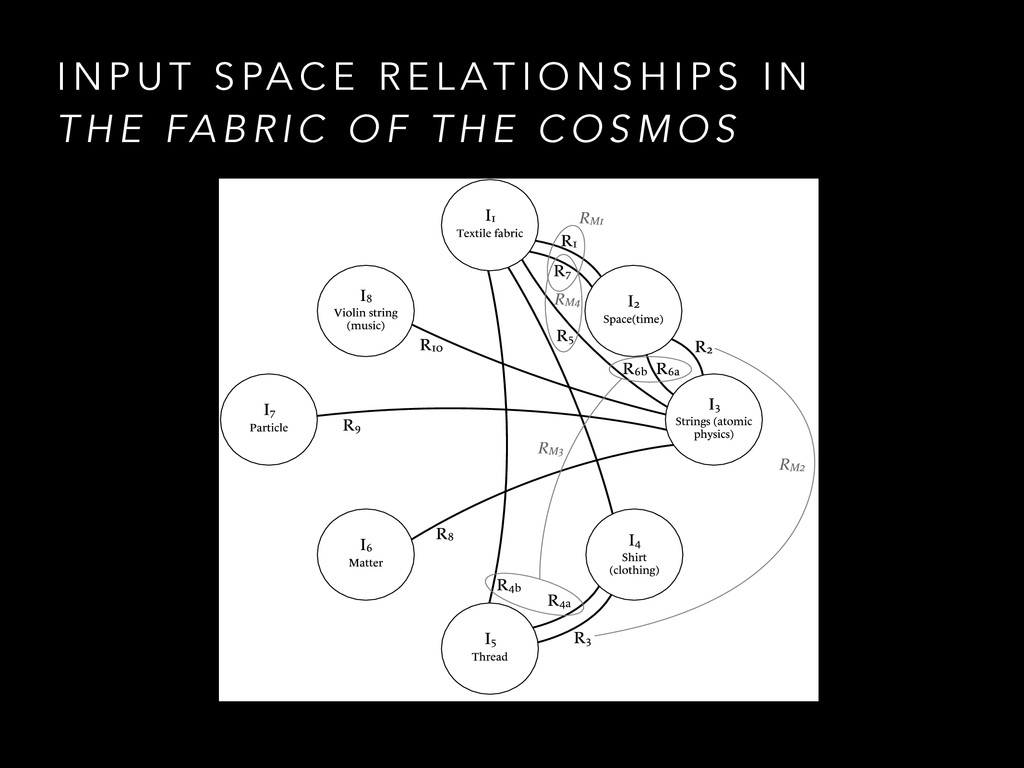
15. FA B R I C O F T H E C O S M O S Since we speak of the ‘fabric’ of spacetime, the suggestion goes, maybe spacetime is stitched out of strings much as a shirt is stitched out of thread. That is, much as joining numerous threads together in an appropriate pattern produces a shirt’s fabric, maybe joining numerous strings together in an appropriate pattern produces what we commonly call spacetime’s fabric. Matter, like you and me, would then amount to additional agglomerations of vibrating strings. Every particle is composed of a tiny filament of energy, some hundred billion billion times smaller than a single atomic nucleus which is shaped like a little string. And just as a violin string can vibrate in different patterns, each of which produces a different musical tone, the filaments of superstring theory can also vibrate in different patterns. Greene, Brian. 2004. The Fabric of the Cosmos. Harmondsworth: Penguin. pp.486-7
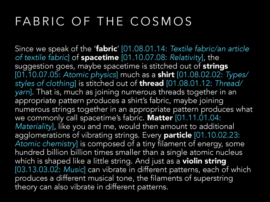
16. Since we speak of the ‘fabric’ [01.08.01.14: Textile fabric/an article of textile fabric] of spacetime [01.10.07.08: Relativity], the suggestion goes, maybe spacetime is stitched out of strings [01.10.07.05: Atomic physics] much as a shirt [01.08.02.02: Types/ styles of clothing] is stitched out of thread [01.08.01.12: Thread/ yarn]. That is, much as joining numerous threads together in an appropriate pattern produces a shirt’s fabric, maybe joining numerous strings together in an appropriate pattern produces what we commonly call spacetime’s fabric. Matter [01.11.01.04: Materiality], like you and me, would then amount to additional agglomerations of vibrating strings. Every particle [01.10.02.23: Atomic chemistry] is composed of a tiny filament of energy, some hundred billion billion times smaller than a single atomic nucleus which is shaped like a little string. And just as a violin string [03.13.03.02: Music] can vibrate in different patterns, each of which produces a different musical tone, the filaments of superstring theory can also vibrate in different patterns. FA B R I C O F T H E C O S M O S
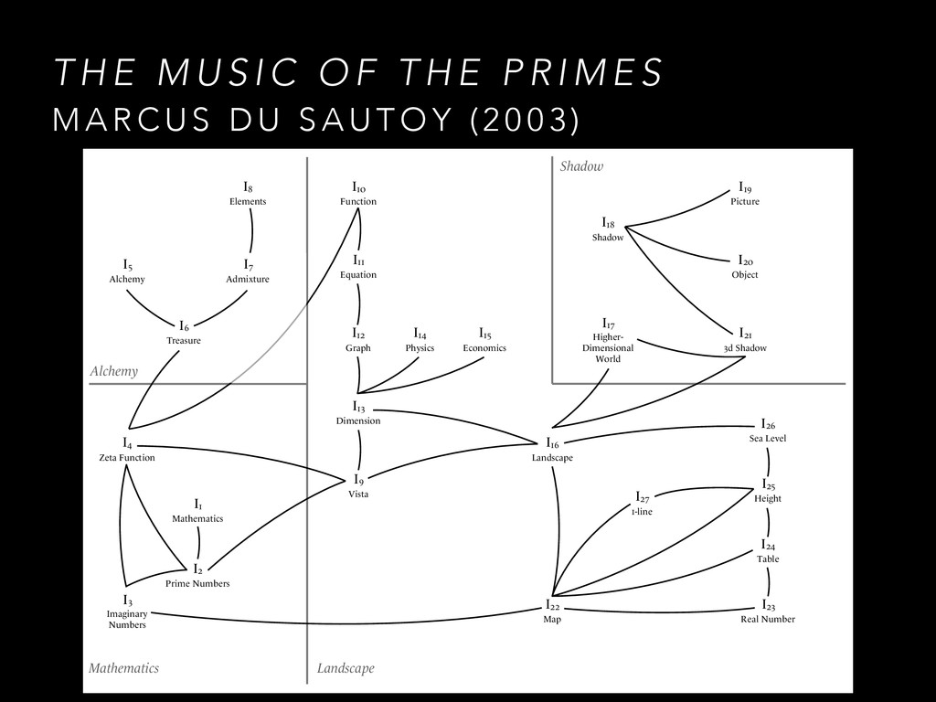
17. M U S I C O F T H E P R I M E S Gauss’s two-dimensional map of imaginary numbers charts the numbers that we shall feed into the zeta function. The north-south axis keeps track of how many steps we take in the imaginary direction, whilst the east west axis charts the real numbers. We can lay this map out flat on a table. What we want to do is to create a physical landscape situated in the space above this map. The shadow of the zeta function will then turn into a physical object whose peaks and valleys we can explore. du Sautoy, Marcus. 2003. The Music of the Primes. London: Harper. p.85
18. Gauss’s two-dimensional map [01.01.09.01: Geography – Map-making] of imaginary numbers [01.16.04 – Number] charts the numbers that we shall feed into the zeta function. The north-south axis [01.16.04.12 – Geometry] keeps track of how many steps [01.14.03.02 – Walking] we take in the imaginary direction [01.12.06 – Direction], whilst the east west axis charts the real numbers. We can lay this map [01.01.09.01: Geography – Map-making] out flat on a table. What we want to do is to create a physical landscape [01.01.04 – Land] situated in the space above this map. The shadow of the zeta function will then turn into a physical object whose peaks [01.01.04.04.01.03 – Hill/mountain] and valleys [01.01.04.04.02.03 – Valley] we can explore. M U S I C O F T H E P R I M E S
19. I N P U T S PA C E R E L A T I O N S H I P S I N 
 T H E FA B R I C O F T H E C O S M O S
20. C O M P R E S S I O N O F I N P U T S PA C E S
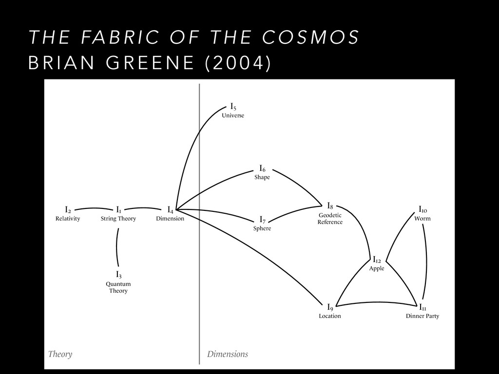
21. T H E FA B R I C O F T H E C O S M O S 
 B R I A N G R E E N E ( 2 0 0 4 ) I2 Relativity I1 String Theory I4 Dimension I3 Quantum Theory I5 Universe I6 Shape I7 Sphere I8 Geodetic Reference I9 Location I12 Apple I11 Dinner Party I10 Worm Theory Dimensions
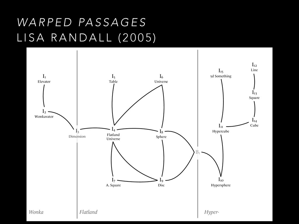
22. WA R P E D PA S S A G E S 
 L I S A R A N D A L L ( 2 0 0 5 ) I2 Wonkavator I1 Elevator I4 Flatland Universe I5 Table I6 Universe I7 A. Square I8 Sphere I9 Disc I15 5d Something I11 Hypercube I10 Hypersphere Wonka Flatland Hyper- I3 Dimension B1 I12 Line I13 Square I14 Cube
23. T H E M U S I C O F T H E P R I M E S 
 M A R C U S D U S A U T O Y ( 2 0 0 3 ) I4 Zeta Function Mathematics I5 Alchemy I6 Treasure I7 Admixture I8 Elements I3 Imaginary Numbers I2 Prime Numbers I1 Mathematics I9 Vista Alchemy Landscape I13 Dimension I12 Graph I11 Equation I10 Function I14 Physics I15 Economics Shadow I17 Higher- Dimensional World I21 3d Shadow I20 Object I19 Picture I18 Shadow I16 Landscape I22 Map I23 Real Number I24 Table I25 Height I26 Sea Level I27 1-line
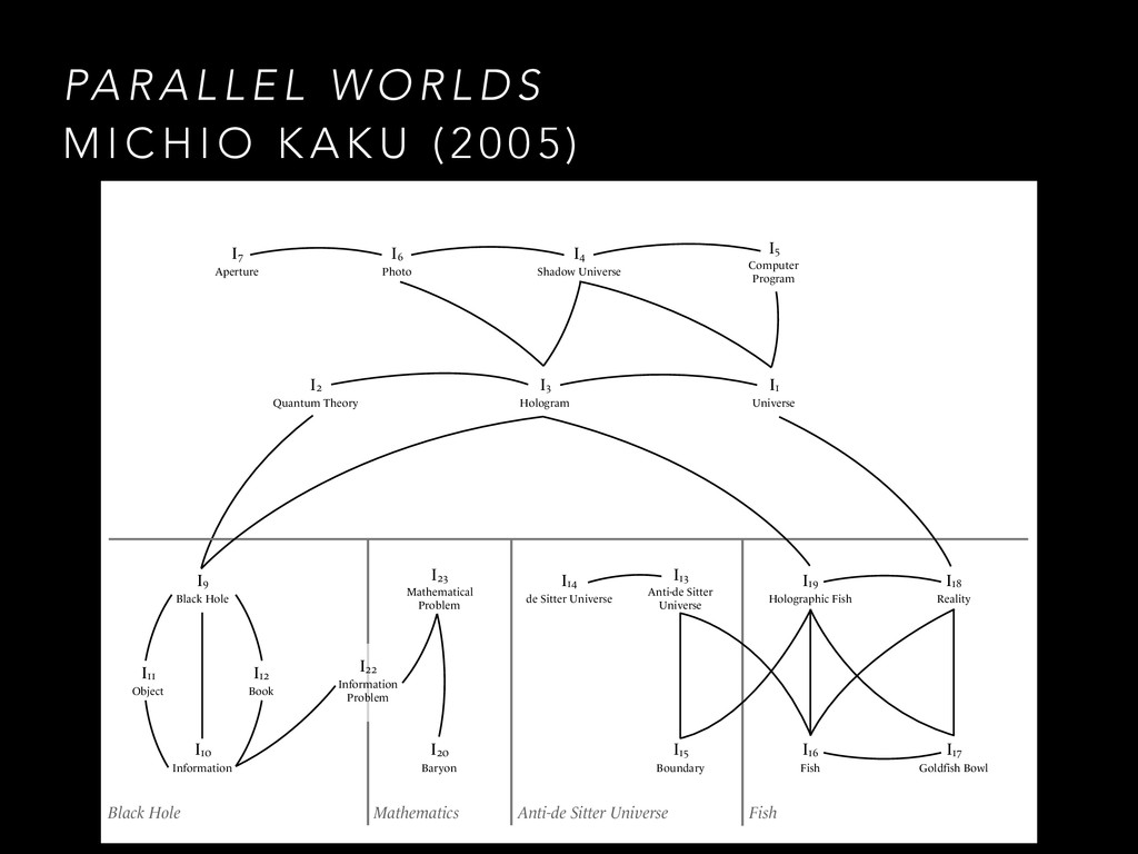
24. PA R A L L E L W O R L D S 
 M I C H I O K A K U ( 2 0 0 5 ) Black Hole I10 Information I14 de Sitter Universe Mathematics Anti-de Sitter Universe Fish I11 Object I12 Book I9 Black Hole I22 Information Problem I20 Baryon I23 Mathematical Problem I15 Boundary I13 Anti-de Sitter Universe I16 Fish I19 Holographic Fish I17 Goldfish Bowl I18 Reality I2 Quantum Theory I3 Hologram I1 Universe I7 Aperture I4 Shadow Universe I5 Computer Program I6 Photo
25. www.glasgow.ac.uk/thesaurus www.glasgow.ac.uk/samuels SAMUELS Web Tagger: http://is.gd/semtag Cover image: Samantha Keeley Smith, Talisman (2012)