Upgrade to Pro — share decks privately, control downloads, hide ads and more …

High dimensional Quasi Monte Carlo in Finance

Marco Bianchetti
May 12, 2016
79

High dimensional Quasi Monte Carlo in Finance

Monte Carlo simulation in finance has been traditionally focused on pricing derivatives. Actually nowadays market and counterparty risk measures, based on multi-dimensional multi-step Monte Carlo simulation, are very important tools for managing risk, both on the front office side (sensitivities, CVA) and on the risk management side (estimating risk and capital allocation). Furthermore, they are typically required for internal models and validated by regulators.
The daily production of prices and risk measures for large portfolios with multiple counterparties is a computationally intensive task, which requires a complex framework and an industrial approach. It is a typical high budget, high effort project in banks.
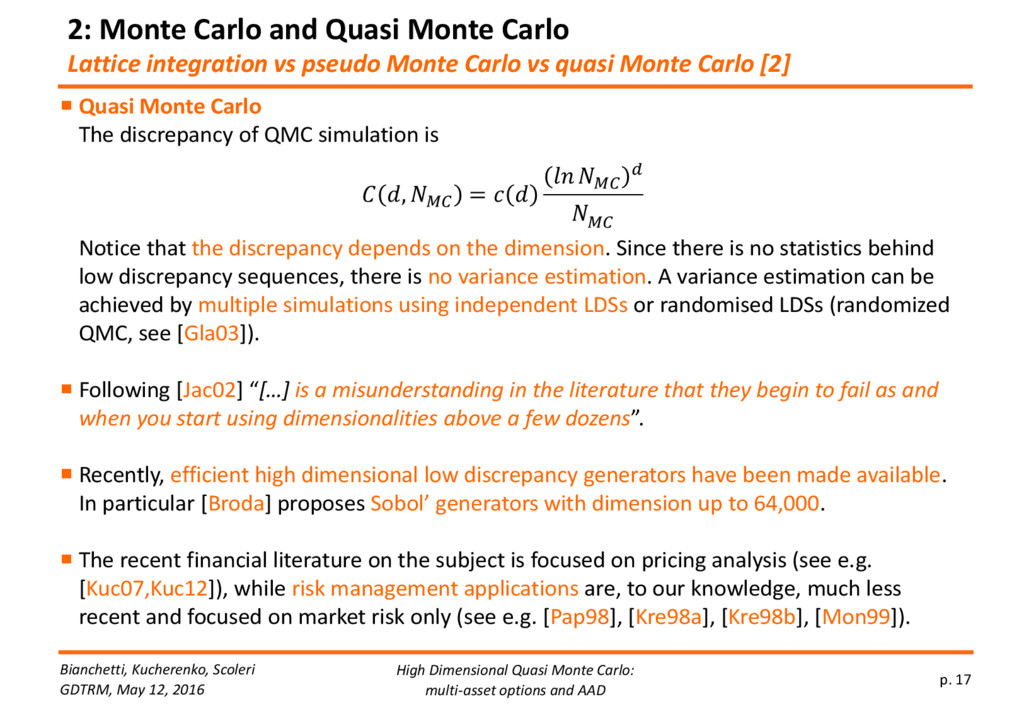
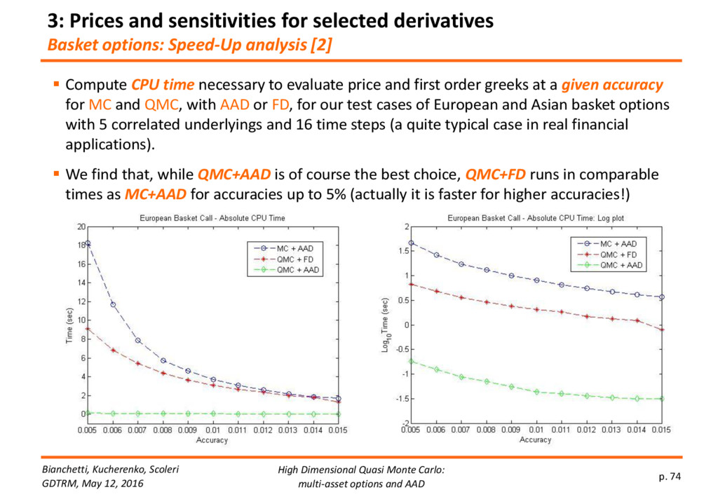
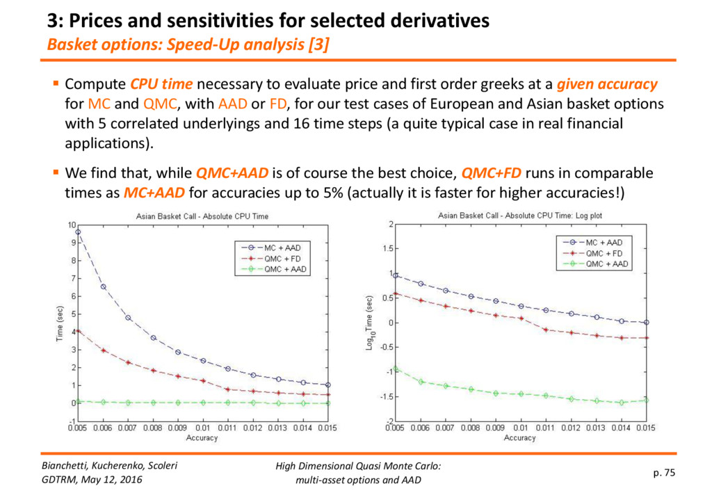
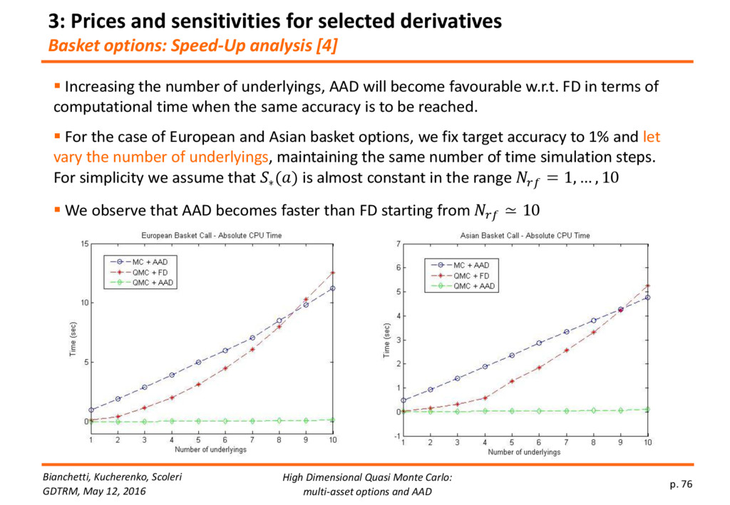
In this presentation we focus on the Monte Carlo simulation, showing that, despite some common wisdom, Quasi Monte Carlo techniques can be applied, under appropriate conditions, to successfully improve price and risk figures and to reduce the computational effort.
This work includes and extends our paper M. Bianchetti, S. Kucherenko and S. Scoleri, “Pricing and Risk Management with High-Dimensional Quasi Monte Carlo and Global Sensitivity Analysis”, Wilmott Journal, July 2015 (also available at http://ssrn.com/abstract=2592753).

Marco Bianchetti

May 12, 2016
Tweet

Transcript

  1. High Dimensional Quasi Monte Carlo Methods: Multi-Asset Options and FD

    vs AAD Greeks Marco Bianchetti, Intesa Sanpaolo, Financial and Market Risk Management Sergei Kucherenko, Imperial College London Stefano Scoleri, Iason Ltd. Global Derivatives Trading and Risk Management, Budapest, May 12, 2016
  2. High Dimensional Quasi Monte Carlo: multi-asset options and AAD p.

    1 Bianchetti, Kucherenko, Scoleri GDTRM, May 12, 2016 Agenda 1. Introduction 2. Monte Carlo and Quasi Monte Carlo o History o Multi-dimensional multi-step MC simulation o Numbers: true random, pseudo random, and low discrepancy o Lattice integration vs Pseudo vs quasi Monte Carlo o Global sensitivity analysis, effective dimensions, error analysis o Adjoint Algorithmic Differentiation 3. Prices and sensitivities for selected derivatives o Numerical results for single-asset derivatives o Numerical results for multi-asset derivatives 4. Exposures for derivatives’ portfolios o Counterparty risk measures o Single option portfolio 5. Market and Counterparty risk of real derivatives’ portfolios o MC simulation for risk measures computation o Numerical results for real cases 6. Conclusions 7. References
  3. High Dimensional Quasi Monte Carlo: multi-asset options and AAD p.

    2 Bianchetti, Kucherenko, Scoleri GDTRM, May 12, 2016 1: Introduction  Monte Carlo simulation in finance has been traditionally focused on pricing derivatives. Actually nowadays market and counterparty risk measures, based on multi-dimensional multi-step Monte Carlo simulation, are very important tools for managing risk, both on the front office side (sensitivities, CVA) and on the risk management side (estimating risk and capital allocation). Furthermore, they are typically required for internal models and validated by regulators.  The daily production of prices and risk measures for large portfolios with multiple counterparties is a computationally intensive task, which requires a complex framework and an industrial approach. It is a typical high budget, high effort project in banks.  We will focus on the Monte Carlo simulation, showing that, despite some common wisdom, Quasi Monte Carlo techniques can be applied, under appropriate conditions, to successfully improve price and risk figures and to reduce the computational effort.  The present work includes and extends our paper M.Bianchetti, S. Kucherenko and S.Scoleri, “Pricing and Risk Management with High-Dimensional Quasi Monte Carlo and Global Sensitivity Analysis”, Wilmott Journal, July 2015 (also available at http://ssrn.com/abstract=2592753).
  4. High Dimensional Quasi Monte Carlo: multi-asset options and AAD p.

    3 Bianchetti, Kucherenko, Scoleri GDTRM, May 12, 2016 2: Monte Carlo and Quasi Monte Carlo History The Monte Carlo method was coined in the 1940s by John von Neumann, Stanislaw Ulam and Nicholas Metropolis, working on nuclear weapons (Manhattan Project) at Los Alamos National Laboratory [JVN51]. Metropolis suggested the name Monte Carlo, referring to the Monte Carlo Casino, where Ulam's uncle often gambled away his money [Met87, Wiki]. Enrico Fermi is suspected to have used some “manual back of the envelope simulation” in the 1930s, working in Rome on nuclear reactions induced by slow neutrons (without publication) [Los66, Met87]. Enrico Fermi Roma, 1901 – Chicago, 1954 John Von Neumann Budapest, 1903 – Washington, 1957 Stanislaw Ulam Leopolis, 1909 – Santa Fe, 1984 Nicholas Metropolis Chicago, 1915 – Los Alamos, 1999
  5. High Dimensional Quasi Monte Carlo: multi-asset options and AAD p.

    4 Bianchetti, Kucherenko, Scoleri GDTRM, May 12, 2016 2: Monte Carlo and Quasi Monte Carlo Other «quasi»  Quasi crystal a structure that is ordered but not periodic. A quasi crystalline pattern can continuously fill all available space, but it lacks translational symmetry (http://en.wikipedia.org/wiki/Quasicrystal).  Quasi particle phenomena that occur when a microscopically system such as a solid behaves as if it contained different weakly interacting particles in free space. For example, the aggregate motion of electrons in the valence band of a semiconductor is the same as if the semiconductor contained instead positively charged quasi particles called “holes”.  Quasi satellite A quasi satellite's orbit around the Sun takes exactly the same time as the planet's, but has a different eccentricity (usually greater).
  6. High Dimensional Quasi Monte Carlo: multi-asset options and AAD p.

    5 Bianchetti, Kucherenko, Scoleri GDTRM, May 12, 2016  The risk factors dynamics are described by stochastic differential equations (SDE) where  is the drift,  is the Nrf x Nrf volatility matrix, and dW is a Nrf – dimensional brownian motion. Model parameters can be calibrated to market quotes (risk neutral world measure) or to historical series (real world measure).  We discretize the future time axis by choosing a time simulation grid t = [t1 ,…,t Nstep ]  The Monte Carlo scenario sjk := sk (tj ) at (discrete) time simulation step tj is a NMC – dimensional (random) draw of standard brownian motions across the time step [tj-1 ,tj ]  The risk factor scenario rijk := rik (tj ,sjk ) is the value of the risk factor ri at time step tj on Monte Carlo scenario sjk 2: Monte Carlo and Quasi Monte Carlo Multi-dimensional multi-step MC simulation [1]
  7. High Dimensional Quasi Monte Carlo: multi-asset options and AAD p.

    6 Bianchetti, Kucherenko, Scoleri GDTRM, May 12, 2016 The MC computation of financial quantities is based, in general, on a multi-dimensional multi- step simulation, proceeding as follows.  for each Monte Carlo scenario sjk • for each time simulation step tj  for each risk factor ri  simulate the risk factor values rijk o for each trade l in the portfolio  compute the mark to future value vjkl o loop over portfolio trades l=1,…,Nptf  loop over risk factors i=1,…,Nrf • loop over time simulation steps j=1,…,Nstep  loop over Monte Carlo scenarios k=1,…,NMC Notice that the mark to future value vjkl may require another MC simulation in itself, depending on the payoff for trade l and on the pricing model assigned to it. In this case we have a nested Monte Carlo simulation. Also a model calibration could be necessary. 2: Monte Carlo and Quasi Monte Carlo Multi-dimensional multi-step MC simulation [2] Risk factor value Mark to future value
  8. High Dimensional Quasi Monte Carlo: multi-asset options and AAD p.

    7 Bianchetti, Kucherenko, Scoleri GDTRM, May 12, 2016  The mark to future is the future value vjkl of the individual trades survived at time step tj .  The portfolio mark to future Vjk is the sum of the future values of all trades in the portfolio (we assume linear combination of trades). The aggregation of trades can follow different rules, for example to accommodate different counterparties with different netting sets. The netting set mark to future Vjkh is the sum of all the trades in the netting set nh subject to the same netting agreement with a given counterparty  Notice that if the l-th trade maturity Tl is smaller than the time simulation step tj , the l-th trade is dead and there is nothing to compute, 2: Monte Carlo and Quasi Monte Carlo Multi-dimensional multi-step MC simulation [3]
  9. High Dimensional Quasi Monte Carlo: multi-asset options and AAD p.

    8 Bianchetti, Kucherenko, Scoleri GDTRM, May 12, 2016  The nominal dimension of the Monte Carlo simulation is (see e.g. [Jac03]) DMC = (n° of risk factors) x (n° of time simulation steps) = Nrf x Nstep  The performance of the Monte Carlo simulation depends on o the number of risk factors Nrf , o the number of time simulation steps Nstep , o the number of MC scenarios NMC , o the properties of (random) numbers  generator, o the speed of convergence of the MC simulation, o the stability of the MC simulation, o the number of trades N and of netting sets Nh in the portfolio, o the computational cost to price each trade with analytical formulas, PDE, or MC simulations, o the dependence of trades on risk factors, o … 2: Monte Carlo and Quasi Monte Carlo Multi-dimensional multi-step MC simulation [4]
  10. High Dimensional Quasi Monte Carlo: multi-asset options and AAD p.

    9 Bianchetti, Kucherenko, Scoleri GDTRM, May 12, 2016  In particular, notice that the (netting set or portfolio) mark to future Vjk at time step tj depends, in principle, on all the risk factors  In practice, each trade and netting set will show an effective dimension ≤ , due to the trade expiration and to hierarchical dependency on risk factors as follows: o higher sensitivity to primary risk factors o smaller sensitivity to secondary risk factors o negligible or null sensitivity to negligible risk factors Primary risk factors Secondary risk factors Negligible risk factors How to take advantage of these features of the problem ? Global Sensitivity Analysis ! 2: Monte Carlo and Quasi Monte Carlo Multi-dimensional multi-step MC simulation [5]
  11. High Dimensional Quasi Monte Carlo: multi-asset options and AAD p.

    10 Bianchetti, Kucherenko, Scoleri GDTRM, May 12, 2016  Random vs deterministic events o Random events are intrinsically unpredictable. o Deterministic events are, in principle, predictable. In practice, it depends on our knowledge. Determinism is the hypothesis that actually there is no randomness in the universe, only unpredictability (that is, our ignorance). o According to the Bayesian interpretation of probability, probability can be used to represent a lack of complete knowledge of events. o Random events are very common in our universe. Some examples: o Radioactive decay of a single unstable nucleus or particle is intrinsically random. Its average lifetime is perfectly deterministic. Think to radiocarbon dating. o Atomic motion in a gas is random. Newton’s equations of motion are deterministic. o Genetic mutations are random. DNA reproduction is deterministic.  True random numbers generators (TRNGs) o Random numbers can be produced by appropriate hardware, called True Random Number Generators (TRNGs), based on statistically random physical processes, such as quantum mechanical effects (e.g. radioactive decay), or thermal noise. o Random numbers cannot be produced by a computer executing deterministic instructions. “Anyone who considers arithmetical methods of producing random digits is, of course, in a state of sin.” (John von Neumann, 1951 *JVN51]). 2: Monte Carlo and Quasi Monte Carlo Numbers: true random
  12. High Dimensional Quasi Monte Carlo: multi-asset options and AAD p.

    11 Bianchetti, Kucherenko, Scoleri GDTRM, May 12, 2016  Pseudo Random Numbers Generators (PRNGs) Pseudo random numbers are generated by algorithms called Pseudo Random Number Generators (PRNGs). PRNGs produce deterministic sequences of numbers that approximates the properties of a random sequences. Such sequences are completely determined by a set of initial values, called the PRNG's state. Thus, sequences produced by PRNGs are reproducible, using the same set of state variables.  Main characteristics of PRNGs: o Seed: the number used to initialize the PRNG. It must be a random number. o Periodicity: the maximum length, over all possible state variables, of the sequence without repetition. o Distribution: distribution of the random numbers generated, generally uniform [0,1).  Most common PRNGs: o Pioneer PRNGs: Mid Square Method by John Von Neumann in 1946 (see [Jac02]). o Classical PRNGs: see e.g. [NR02] and [Jac02]. o Mersenne Twister: the best at the moment, with the longest period of 106000 iterations. See [MT97,JAC02].  Main lessons: o all PRNGs are flawed by definition. o know your PRNG: seed, periodicity, limits, etc., never use it as a black box. 2: Monte Carlo and Quasi Monte Carlo Numbers: pseudo random
  13. High Dimensional Quasi Monte Carlo: multi-asset options and AAD p.

    12 Bianchetti, Kucherenko, Scoleri GDTRM, May 12, 2016  Low Discrepancy Numbers or Quasi Random Numbers (QRN), are such that any sequence of these numbers has low discrepancy. Formally, a sequence of d-dimensional numbers in [0,1]d, has low discrepancy if the first N points {u1 ,...,uN } in the sequence satisfy where D is the discrepancy and c(d) is some constant depending only on d. The key point is that low discrepancy is required for any subsequence with N > 1, not for some fixed N.  The discrepancy of a sequence {u1 ,...,uN } is a measure of how inhomogeneously the sequence is distributed inside the unit hypercube Id=[0,1]d. Formally 2: Monte Carlo and Quasi Monte Carlo Numbers: low discrepancy [1] Discrepancy Sub-hypercube Number of draws in Sd
  14. High Dimensional Quasi Monte Carlo: multi-asset options and AAD p.

    13 Bianchetti, Kucherenko, Scoleri GDTRM, May 12, 2016 2: Monte Carlo and Quasi Monte Carlo Numbers: low discrepancy [2] The first 1024 points of two-dimensional Sobol sequence. At each stage, the new points regularly fill the gaps in the distribution generated at the previous stage. Source: Numerical Recipes [NR02] The first 256 points from a PRNG (top) compared with the first 256 points from the 2,3 Sobol sequence (bottom). The Sobol sequence covers the space more evenly (red=1,..,10, blue=11,..,100, green=101,..,256). Source: [Wikipedia]. Notice how the discrepancy of the sequence of N QRNs is minimized for each sub-sequence n=1,…,N, with respect to the PRNs.
  15. High Dimensional Quasi Monte Carlo: multi-asset options and AAD p.

    14 Bianchetti, Kucherenko, Scoleri GDTRM, May 12, 2016 2: Monte Carlo and Quasi Monte Carlo Numbers: low discrepancy [3]  Low Discrepancy Numbers Generators (LDNGs): as for PRNGs, there are many algorithms to produce low discrepancy numbers, the most important being (see e.g. [Jac02], [Gla03]): o Van der Corput numbers o Halton numbers o Faure numbers o Sobol` numbers  Sobol` Numbers o use a base of 2 to form successively finer uniform partitions of the unit interval, and then reorder the coordinates in each dimension. o The number of iterations should be taken as N=2n for n integer. o Once well-initialised, they provide :  the lowest discrepancy in lower dimensions  comparable discrepancy with pseudo random numbers in higher dimensions L2 norm discrepancy (y-axis) as a function of the number of iterations (x-axis) for various PRNGs and LDNGs, in dimension d=2 (up) and d=100 (down). Source: [Jac02]. Ilya Sobol’ Moscow , 1926 –
  16. High Dimensional Quasi Monte Carlo: multi-asset options and AAD p.

    15 Bianchetti, Kucherenko, Scoleri GDTRM, May 12, 2016  Uniform NGs Standard NGs produce numbers with a continuous uniform distribution U[a,b], such that the probability density function f is constant over the interval [a,b],  Non uniform RNGs Numbers with any distribution with probability density f(x) can be produced, in principle, starting from the uniform distribution U[0,1] by inverting the following relation because the cumulative probability function F(x) is a probability measure, which is uniform on [0,1] by definition. Given a number y with uniform distribution U(0,1) we obtain See e.g. [NR02], [Jac02] and [Gla03] for (a lot of) details. 2: Monte Carlo and Quasi Monte Carlo Numbers: distribution
  17. High Dimensional Quasi Monte Carlo: multi-asset options and AAD p.

    16 Bianchetti, Kucherenko, Scoleri GDTRM, May 12, 2016 2: Monte Carlo and Quasi Monte Carlo Lattice integration vs pseudo Monte Carlo vs quasi Monte Carlo [1]  Lattice integration The numerical integration of a given d-dimensional function on a regular grid with Nlattice points in the hypercube domain of volume Ld has a relative error  Pseudo Monte Carlo The standard error associated to PMC, by the central limit theorem, is where 2 is the estimated variance of the simulation. Variance reduction techniques, e.g. antithetic variables, affect only the numerator [Gla03].
  18. High Dimensional Quasi Monte Carlo: multi-asset options and AAD p.

    17 Bianchetti, Kucherenko, Scoleri GDTRM, May 12, 2016 2: Monte Carlo and Quasi Monte Carlo Lattice integration vs pseudo Monte Carlo vs quasi Monte Carlo [2]  Quasi Monte Carlo The discrepancy of QMC simulation is Notice that the discrepancy depends on the dimension. Since there is no statistics behind low discrepancy sequences, there is no variance estimation. A variance estimation can be achieved by multiple simulations using independent LDSs or randomised LDSs (randomized QMC, see [Gla03]).  Following [Jac02+ “[…] is a misunderstanding in the literature that they begin to fail as and when you start using dimensionalities above a few dozens”.  Recently, efficient high dimensional low discrepancy generators have been made available. In particular [Broda] proposes Sobol’ generators with dimension up to 64,000.  The recent financial literature on the subject is focused on pricing analysis (see e.g. [Kuc07,Kuc12]), while risk management applications are, to our knowledge, much less recent and focused on market risk only (see e.g. [Pap98], [Kre98a], [Kre98b], [Mon99]).
  19. High Dimensional Quasi Monte Carlo: multi-asset options and AAD p.

    18 Bianchetti, Kucherenko, Scoleri GDTRM, May 12, 2016 2: Monte Carlo and Quasi Monte Carlo Global sensitivity analysis [1] Input variables Model function Output variable Without loss of generality we can take VD to be the D-dimensional hypercube, so that Advantages of GSA w.r.t. other SA approaches: o Standard SA quantifies the effect of varying a given input (or set of inputs) while all other inputs are kept constant. o GSA quantifies the effect of varying a given input (or set of inputs) while all other inputs are varied as well. Thus, it provides a measure of interaction among variables. It can be applied also to non-linear models.  Risk measures: o D = Nrf x Nstep (can be very high!) o y = portfolio P&L (VaR, ES), portfolio value (EPE/ENE, PFE)  Option pricing: o D = Nstep (single asset) o D = Nrf x Nstep (multiple assets) o y = Price, Greeks
  20. High Dimensional Quasi Monte Carlo: multi-asset options and AAD p.

    19 Bianchetti, Kucherenko, Scoleri GDTRM, May 12, 2016 2: Monte Carlo and Quasi Monte Carlo Global sensitivity analysis [2]  ANOVA decomposition Under appropriate regularity conditions, the decomposition is unique if In this case terms are orthogonal and are given by integrals involving only f(x). For square integrable functions, the total variance of f decomposes as Partial variances First order terms Second order terms D-order term
  21. Better Pricing and Risk Management with High Dimensional Quasi Monte

    Carlo p. 20 Bianchetti, Kucherenko, Scoleri WBS 10th Fixed Income Conference 2: Monte Carlo and Quasi Monte Carlo Global sensitivity analysis [3]  Sobol’ sensitivity indices o They measure the fraction of variance accounted by 1,…, 1 , … , o They sum up to 1 o For s>1 they measure interactions among 1 , … , o One can introduce Sobol’ indices for subsets of variables in order to measure the importance of a subset y of x w.r.t. the complementary subset z. Moreover, one can introduce total effect indices in order to measure the total contribution of a subset y to the total variance [Sob05b]. They can be used to: o Rank variables in order of importance o Fix unessential variables o Reduce model complexity o Analyze/predict the efficiency of various numerical schemes
  22. High Dimensional Quasi Monte Carlo: multi-asset options and AAD p.

    21 Bianchetti, Kucherenko, Scoleri GDTRM, May 12, 2016 2: Monte Carlo and Quasi Monte Carlo Global sensitivity analysis [4]  The most used Sobol’ sensitivity indices in practice are  Special cases are: o = 0: the output function doesn’t depend on o = 1: the output function depends only on o = : interactions between and other variables are absent
  23. High Dimensional Quasi Monte Carlo: multi-asset options and AAD p.

    22 Bianchetti, Kucherenko, Scoleri GDTRM, May 12, 2016 2: Monte Carlo and Quasi Monte Carlo Global sensitivity analysis [5]  Sobol’ indices are expressed as high-dimensional integrals, so they are usually evaluated via MC/QMC techniques. Efficient formulas have been developed, which allow to compute Sobol’ indices for subsets of variables directly from f(x) , thus avoiding the knowledge of ANOVA components [Sob05b]. Furthermore, the computation of and can be reduced to ( + 2) function evaluations [Kuc11], where y and z (or y’ and z’) are two complementary subsets of x (or x’).
  24. High Dimensional Quasi Monte Carlo: multi-asset options and AAD p.

    23 Bianchetti, Kucherenko, Scoleri GDTRM, May 12, 2016 2: Monte Carlo and Quasi Monte Carlo Effective dimensions [1]  Many financial problems are high-dimensional, but often not all the variables are equally important: effective dimensions were introduced to quantitatively measure the number of most important variables of a model function [Caf97] .  The superior efficiency of QMC methods for some high-dimensional problems can be ascribed to a reduced effective dimension w.r.t. nominal dimension of the model function f(x).  GSA can be used to compute effective dimensions and, thus, to predict the performance of QMC method w.r.t. standard MC, for a given f(x).  Different notions of effective dimensions can be introduced: o The effective dimension in the superposition sense is the smallest dS such that o The effective dimension in the truncation sense is the smallest dT such that o The average dimension dA is defined as = 0< <
  25. High Dimensional Quasi Monte Carlo: multi-asset options and AAD p.

    24 Bianchetti, Kucherenko, Scoleri GDTRM, May 12, 2016 2: Monte Carlo and Quasi Monte Carlo Effective dimensions [2]  The effective dimension in superposition sense dS does not depend on the order of sampling of variables, while the effective dimensionin the truncation sense dT does.  The following inequality holds: ≤ .  All high-dimensional numerical experiments found in the literature show that QMC is more efficient than MC when the effective dimension (in one or more senses) is small. In particular [Sob14] suggests that QMC could be more efficient than MC when ≾ 3  Functions f(x) can be classified according to their dependence on variables: For Type A and Type B functions, QMC is more efficient than MC, for Type C functions QMC cannot achieve higher accuracy than MC. Type A and Type B functions are very common in financial problems, possibly after effective dimension reduction.
  26. High Dimensional Quasi Monte Carlo: multi-asset options and AAD p.

    25 Bianchetti, Kucherenko, Scoleri GDTRM, May 12, 2016 2: Monte Carlo and Quasi Monte Carlo Effective dimensions [3]  Contrary to MC, QMC efficiency is sensitive to the order in which variables x are sampled from the LDS. The common explanation is that, since lower coordinates in each D- dimensional LDS draw are particularly well distributed, one should use them to simulate the most important variables and concentrate there most of the variance. Moreover, since lower dimensional projections of LDS (especially for well initialized Sobol’ sequences) are much better distributed, in the case of Type B functions, higher-order interaction terms should be relegated to later dimension, whose projections are not so well distributed.  The optimal sampling order is not a priori known for a given f(x). In path-dependent option pricing, a popular choice is to apply Brownian Bridge to the discretization of the underlying stochastic process [Caf97]. Some authors report cases where Brownian Bridge is not superior to standard discretization [Pap01]. Other discretization schemes are possible.  GSA explains why a given discretization scheme improves QMC convergence and can predict its superiority to MC, at a reasonable computational cost, without actually computing the convergence rate via direct simulations (which would be very time-consuming).
  27. High Dimensional Quasi Monte Carlo: multi-asset options and AAD p.

    26 Bianchetti, Kucherenko, Scoleri GDTRM, May 12, 2016 2: Monte Carlo and Quasi Monte Carlo Error Analysis Many problems in financial engineering can be reduced to high-dimensional integration of a given function f, hence MC/QMC simulation is usually the election method to solve them.  In order to measure the efficiency of the two techniques, the integration error  as a function of the number of simulated paths NMC is analysed.  If V is the exact value of the integral and VN is the simulated value using N paths, the root mean square error, averaged on L independent runs, is defined as In the MC case, L=1. In the QMC case, for each run, a different part of the LDS is used.  In order to compare the performances of the two techniques we conduct the three following analyses: A. Convergence analysis B. Monotonicity and stability analysis C. Speed-up analysis
  28. High Dimensional Quasi Monte Carlo: multi-asset options and AAD p.

    27 Bianchetti, Kucherenko, Scoleri GDTRM, May 12, 2016 2: Monte Carlo and Quasi Monte Carlo Error Analysis: convergence A. Convergence analysis  MC convergence rate is known to be irrespective of the dimensionality  An upper bound to QMC convergence rate is log . It is asymptotically faster than MC but it depends on dimensionality and, for feasible N, it can be too slow. However, it is not observed in practice: integrands with low effective dimension show faster convergence: with approaching 1.  The root mean square error can be computed for different numbers of simulated paths and constants c and  can be estimated from linear regression.
  29. High Dimensional Quasi Monte Carlo: multi-asset options and AAD p.

    28 Bianchetti, Kucherenko, Scoleri GDTRM, May 12, 2016 2: Monte Carlo and Quasi Monte Carlo Error Analysis: monotonicity and stability B. Monotonicity and stability analysis  Numerical tests present in the literature show that QMC convergence is often smoother than MC: such monotonicity and stability guarantee higher accuracy for a given NMC .  In order to quantify monotonicity and stability we adopt the following strategy: 1. divide the range of path simulations in n windows, 2. compute sample mean and sample variance for each window, 3. we propose: o “log-returns” as a measure of monotonicity, and o “volatility” as a measure of stability.  In this way: o Monotonic convergence will show non oscillating log-return converging to zero o Stable convergence will show low and almost flat volatility
  30. High Dimensional Quasi Monte Carlo: multi-asset options and AAD p.

    29 Bianchetti, Kucherenko, Scoleri GDTRM, May 12, 2016 2: Monte Carlo and Quasi Monte Carlo Error Analysis: speed-up C. Speed-up analysis  Such measure is sometimes considered in the literature [Kre98a]. It allows to quantify the computational gain of a method A with respect to a method B.  It is defined as where ∗ is the threshold number of paths needed to reach and maintain a given accuracy a. Speed-Up can be either computed by direct simulation (but it is extremely computationally expensive) or extrapolated from the estimated law of the convergence rate (but it wouldn’t capture unexpected fluctuations due to possible instability).  We choose to identify the threshold ∗ as the estimated N such that
  31. High Dimensional Quasi Monte Carlo: multi-asset options and AAD p.

    30 Bianchetti, Kucherenko, Scoleri GDTRM, May 12, 2016 2: Monte Carlo and Quasi Monte Carlo Adjoint Algorithmic Differentiation [1]  Sensitivities, or Greeks are very important quantities which need to be computed besides price both on the Front Office side (for hedging purposes) and on Risk Management (to monitor the risk of a portfolio w.r.t. specific risk factors).  They are defined as derivatives of the price function w.r.t. risk factors.  Standard techniques (Finite Differences, FD) require bumping each risk factor and re- pricing the instrument on each MC path. The computational cost, therefore, increases linearly with the number of parameters, and becomes particularly expensive for options on multiple underlyings!  One popular alternative to finite differences is Adjoint Algorithmic Differentiation (AAD): it is based on the “Pathwise Derivative” method: unbiased estimators of the Greeks are obtained by differentiating the discounted payoff along each MC path (see [Gla03]). This method can be applied only if the following conditions are satisfied: o the pathwise derivative exists with probability 1 o the payoff is regular enough (e.g. Lipschitz-continuous).  If we want to compute the gradient of a single output w.r.t. many variables (as in the case of Greeks of multi-asset options), the adjoint mode of algorithmic differentiation can be employed to dramatically increase the efficiency of pathwise differentiation.
  32. High Dimensional Quasi Monte Carlo: multi-asset options and AAD p.

    31 Bianchetti, Kucherenko, Scoleri GDTRM, May 12, 2016 2: Monte Carlo and Quasi Monte Carlo Adjoint Algorithmic Differentiation [2] Let Y be a scalar function : ℝ → ℝ, = , = 1 , … , , AAD computation of its partial derivatives works as follows: o Forward Sweep: the output function Y is computed forward from the inputs 1 , … , storing all information at each elementary stage in intermediate variables. o Backward Sweep: by making repeated use of the chain rule, the derivatives of all intermediate variables (i.e. the adjoints) are propagated backward from the output Y to the inputs 1 , … , until the whole gradient is altogether obtained where  AAD provides the full gradient of a function at a cost which is up to 4 times the computational cost of evaluating the function itself, independently of the number of variables.  There exist AD tools which automatically implement the adjoint counterpart of a given computer code.
  33. High Dimensional Quasi Monte Carlo: multi-asset options and AAD p.

    32 Bianchetti, Kucherenko, Scoleri GDTRM, May 12, 2016 2: Monte Carlo and Quasi Monte Carlo Adjoint Algorithmic Differentiation [3] AAD optimizes, in general, the computation of derivatives when we have many inputs and few outputs. Application to Delta and Vega computation of multi-asset options:
  34. High Dimensional Quasi Monte Carlo: multi-asset options and AAD p.

    33 Bianchetti, Kucherenko, Scoleri GDTRM, May 12, 2016 2: Monte Carlo and Quasi Monte Carlo Adjoint Algorithmic Differentiation [4] Pros of AAD: o It is extremely fast, independently of the number of derivatives to compute. Cons of AAD: o It is harder to implement than Finite Differences. o It is not always applicable: in particular it cannot handle discontinuous payoffs. One must regularize the payoff by explicitly smoothing the discontinuity (e.g. approximating a digital call with a call spread or something smoother) or using conditional expectations (e.g. smoothing payoffs with barriers). However this introduces a bias and the use of automatic tools is not straightforward, so that extra effort is needed. o Second order Greeks (Gamma, Vanna, Volga) do not have the benefits of the adjoints for multi-asset options. One usually is forced to use a mixed approach AAD+FD. Recently, also a mixed approach AAD + Likelihood Ratio Method has been proposed [Cap14].
  35. High Dimensional Quasi Monte Carlo: multi-asset options and AAD p.

    34 Bianchetti, Kucherenko, Scoleri GDTRM, May 12, 2016 Agenda 1. Introduction 2. Monte Carlo and Quasi Monte Carlo o History o Multi-dimensional multi-step MC simulation o Numbers: true random, pseudo random, and low discrepancy o Lattice integration vs Pseudo vs quasi Monte Carlo o Global sensitivity analysis, effective dimensions, error analysis o Adjoint Algorithmic Differentiation 3. Prices and sensitivities for selected derivatives o Numerical results for single-asset derivatives o Numerical results for multi-asset derivatives 4. Exposures for derivatives’ portfolios o Counterparty risk measures o Single option portfolio 5. Market and Counterparty risk of real derivatives’ portfolios o MC simulation for risk measures computation o Numerical results for real cases 6. Conclusions 7. References
  36. High Dimensional Quasi Monte Carlo: multi-asset options and AAD p.

    35 Bianchetti, Kucherenko, Scoleri GDTRM, May 12, 2016 3: Prices and sensitivities for selected derivatives Selected payoffs: single assets The aim of this analysis is to compare the efficiency of QMC w.r.t. PMC in computing prices and greeks (Delta, Gamma, Vega) for selected payoffs P with increasing degrees of complexity, using simple dynamical models. In particular we rely on Black-Scholes model, where the underlying assets follows geometric Brownian motions.  European Call:  Asian Call:  Double Knock-Out:  Cliquet: where K is the strike price, = the maturity , and Bu the values of the lower and upper barrier, respectively, C a local cap and F a global floor. The underlying process is discretized across D simulation dates (remember that in the single asset case the number of time simulations steps is equal to the dimension of the MC simulation.)
  37. High Dimensional Quasi Monte Carlo: multi-asset options and AAD p.

    36 Bianchetti, Kucherenko, Scoleri GDTRM, May 12, 2016 3: Prices and sensitivities for selected derivatives Selected payoffs: multiple assets In the multi-asset case, we consider the problem of pricing and hedging the following types of options on multiple underlyings:  European Basket Call:  Asian Basket Call:  Digital Basket Call: where K is the strike price, = the maturity, is the Heaviside function and is the value, at time , of a basket composed of underlyings with weights (recall that, in the multi-asset case, the dimension of the MC simulation is the product of the number of time simulations steps and of the number of underlying assets).
  38. High Dimensional Quasi Monte Carlo: multi-asset options and AAD p.

    37 Bianchetti, Kucherenko, Scoleri GDTRM, May 12, 2016 3: Prices and sensitivities for selected derivatives Simulation details  Prices are computed as averages of the payoff value over NMC scenarios of the underlying process S . The latter are generated according to the following methods: o MC: Mersenne Twister generator [MT98] o QMC: SobolSeq generator [Broda] o NMC scenarios as a power of two, to maximise the efficiency of Sobol’ LDS  Brownian motions are discretized on time steps according to the following schemes: o Standard Discretization: o Brownian Bridge: o Principal Component Analysis for the covariance matrix of [ 1 , … , ( )]  The covariance matrix of the underlying assets can be factorized with: o Cholesky method o Principal Component Analysis
  39. High Dimensional Quasi Monte Carlo: multi-asset options and AAD p.

    38 Bianchetti, Kucherenko, Scoleri GDTRM, May 12, 2016 3: Prices and sensitivities for selected derivatives Simulation details  Greeks are computed via two alternative approaches: o FD: central differences with common PRN/LDS for both base and bumped scenarios o AAD: hand-coded approach to adjoint computation  Quasi Monte Carlo simulation is performed both in the “naïve” way (standard discretization and no reordering of variables) and in the “optimal” way (rearranging the order of variables according to GSA results).  The latter is aimed to increase QMC efficiency by reserving the most important variables to better distributed coordinates of the Sobol’ sequence. This can be achieved with different sampling strategies: BB or PCA along time direction, Cholesky or PCA in risk factors space.  The root mean square error is computed as an average over L independent runs (using non-overlapping LDS) w.r.t. a reference value: the latter is given by analytical formulas, when available, or by a simulated value using a sufficiently large (108 − 109) number of MC scenarios.  Codes are implemented in MATLAB.
  40. High Dimensional Quasi Monte Carlo: multi-asset options and AAD p.

    39 Bianchetti, Kucherenko, Scoleri GDTRM, May 12, 2016 3: Prices and sensitivities for selected derivatives European Call: set up The first test case we consider regards an ATM European call option. Test #1 specs  Risk-free rate: r = 0.03  Spot price: 0 = 100  Volatility: = 0.3  Maturity: T = 1  Strike price: K = 100  Number of time steps: = 32  Output values: Price, Delta, Gamma, Vega  Number of MC/QMC trials for the computation of SI: = 105  Number of simulated paths: = 2, = 9, … , 18  Number of independent runs: L = 30  Increment on finite differences: o 0 = 0 , = 10−4, 10−3, 10−2 o = , = 10−4, 10−3, 10−2
  41. High Dimensional Quasi Monte Carlo: multi-asset options and AAD p.

    40 Bianchetti, Kucherenko, Scoleri GDTRM, May 12, 2016 3: Prices and sensitivities for selected derivatives European Call: global sensitivity analysis [1] GSA for Standard Discretization Price, Delta and Vega are Type- B functions: in these cases we expect that QMC will outperform MC. Gamma is a Type-C function: in this case we expect that QMC won’t outperform MC.
  42. High Dimensional Quasi Monte Carlo: multi-asset options and AAD p.

    41 Bianchetti, Kucherenko, Scoleri GDTRM, May 12, 2016 3: Prices and sensitivities for selected derivatives European Call: global sensitivity analysis [2] GSA for BB Discretization Price, Delta, Gamma and Vega are Type-A functions: we expect that QMC will always outperform MC. Effective dimensions equal 1: this is a trivial result, since the payoff explicitly depends only on one variable (spot at maturity)
  43. High Dimensional Quasi Monte Carlo: multi-asset options and AAD p.

    42 Bianchetti, Kucherenko, Scoleri GDTRM, May 12, 2016 3: Prices and sensitivities for selected derivatives European Call: Error Analysis Speed-up analysis QMC + BB yields speed-ups up to hundreds, especially if higher accuracy is needed From log-log plots of error vs number of simulated paths, one can see that QMC always outperforms MC: in particular, for BB discretization, the root mean square error has lower intercept and slope. It scales with the number of paths approximately as −1.
  44. High Dimensional Quasi Monte Carlo: multi-asset options and AAD p.

    43 Bianchetti, Kucherenko, Scoleri GDTRM, May 12, 2016 3: Prices and sensitivities for selected derivatives European Call: Convergence Analysis For Price, Delta and Vega, QMC + BB converges faster than MC and is much more stable
  45. High Dimensional Quasi Monte Carlo: multi-asset options and AAD p.

    44 Bianchetti, Kucherenko, Scoleri GDTRM, May 12, 2016 3: Prices and sensitivities for selected derivatives Asian Call: set up The second test case regards an ATM geometric average Asian call option. Test #2 specs  Risk-free rate: r = 0.03  Spot price: 0 = 100  Volatility: = 0.3  Maturity: T = 1  Strike price: K = 100  Number of time steps: = 32  Output values: Price, Delta, Gamma, Vega  Number of MC/QMC trials for the computation of SI: = 105  Number of simulated paths: = 2, = 9, … , 18  Number of independent runs: L = 30  Increment on finite differences: o 0 = 0 , = 10−4, 10−3, 10−2 o = , = 10−4, 10−3, 10−2
  46. High Dimensional Quasi Monte Carlo: multi-asset options and AAD p.

    45 Bianchetti, Kucherenko, Scoleri GDTRM, May 12, 2016 3: Prices and sensitivities for selected derivatives Asian Call: global sensitivity analysis [1] GSA for Standard Discretization Price and Vega are Type-A functions. In the case of Delta, some higher-order interactions among variables are present, since for some i. In these cases we expect that QMC will outperform MC (perhaps not too much for Delta). Gamma is a Type-C function: in this case we expect that QMC won’t outperform MC.
  47. High Dimensional Quasi Monte Carlo: multi-asset options and AAD p.

    46 Bianchetti, Kucherenko, Scoleri GDTRM, May 12, 2016 3: Prices and sensitivities for selected derivatives Asian Call: global sensitivity analysis [2] GSA for BB Discretization Price, Delta and Vega are Type- A functions. Variables are not equally important, so that a significant reduction in effective dimension in the truncation sense can be achieved. In these cases we expect that QMC will outperform MC. Gamma is still a Type-C function: in this case we expect that QMC won’t outperform MC.
  48. High Dimensional Quasi Monte Carlo: multi-asset options and AAD p.

    47 Bianchetti, Kucherenko, Scoleri GDTRM, May 12, 2016 3: Prices and sensitivities for selected derivatives Asian Call: Error Analysis Speed-up analysis QMC + BB yields speed-ups from 10 to 100 for Price and Vega, much less for Delta From log-log plots of error vs number of simulated paths, one can see that QMC outperforms MC, even though this is less evident for Delta. For BB discretization, the root mean square error scaling law approaches −1 for Price and Vega, while it is −0.6 for Delta and −0.5 for Gamma.
  49. High Dimensional Quasi Monte Carlo: multi-asset options and AAD p.

    48 Bianchetti, Kucherenko, Scoleri GDTRM, May 12, 2016 3: Prices and sensitivities for selected derivatives Asian Call: Convergence Analysis For Price, (Delta) and Vega, QMC + BB converges faster than MC and is more stable
  50. High Dimensional Quasi Monte Carlo: multi-asset options and AAD p.

    49 Bianchetti, Kucherenko, Scoleri GDTRM, May 12, 2016 3: Prices and sensitivities for selected derivatives Asian Call: Monotonicity and Stability analysis [1] D = 32, BB discretization: MC (blue) vs pure QMC (red) vs randomized QMC (green) QMC is highly monotonic for Price and Vega. Pure QMC is more stable than randomized QMC for Delta and Gamma: higher order interactions decrease monotonicity/stability? Log-returns (up) and volatility (down) for Price, Delta, Gamma and Vega.
  51. High Dimensional Quasi Monte Carlo: multi-asset options and AAD p.

    50 Bianchetti, Kucherenko, Scoleri GDTRM, May 12, 2016 3: Prices and sensitivities for selected derivatives Asian Call: Monotonicity and Stability analysis [2] D = 252, Std vs BB discretization: pure QMC (Std: blue, BB: red) vs randomized QMC (Std: green, BB: pink) When effective dimension is low, i.e. with Brownian Bridge discretization, pure QMC with BRODA generator is always more monotonic and more stable. Log-returns (up) and volatility (down) for Price, Delta, Gamma and Vega.
  52. High Dimensional Quasi Monte Carlo: multi-asset options and AAD p.

    51 Bianchetti, Kucherenko, Scoleri GDTRM, May 12, 2016 3: Prices and sensitivities for selected derivatives Double knock-out barrier option: set up The third test case regards an ATM double knock-out call option. Test #3 specs  Risk-free rate: r = 0.03  Spot price: 0 = 100  Volatility: = 0.3  Maturity: T = 1  Strike price: K = 100  Number of time steps: = 32  Lower barrier: = 0.5 0  Upper barrier: = 1.5 0  Output values: Price, Delta, Gamma, Vega  Number of MC/QMC trials for the computation of SI: = 105  Number of simulated paths: = 2, = 9, … , 18  Number of independent runs: L = 30  Increment on finite differences: o 0 = 0 , = 10−4, 10−3, 10−2 o = , = 10−4, 10−3, 10−2
  53. High Dimensional Quasi Monte Carlo: multi-asset options and AAD p.

    52 Bianchetti, Kucherenko, Scoleri GDTRM, May 12, 2016 3: Prices and sensitivities for selected derivatives Double knock-out barrier option: global sensitivity analysis [1] GSA for Standard Discretization Some higher-order interactions among variables are present in any case, even though the effective dimension in the superposition sense could be slightly reduced for Price and Delta. Interactions appear to decrease while approaching maturity, for Price, Delta and Vega. Gamma and Vega are Type-C function: in these cases QMC won’t outperform MC.
  54. High Dimensional Quasi Monte Carlo: multi-asset options and AAD p.

    53 Bianchetti, Kucherenko, Scoleri GDTRM, May 12, 2016 3: Prices and sensitivities for selected derivatives Double knock-out barrier option: global sensitivity analysis [2] GSA for BB Discretization Price, Delta and Gamma are Type-A functions: they show highly reduced effective dimensions since few variables are important. QMC is expected to outperform MC in these cases. Vega is a Type-C function, even though the average dimension is not too high: in this case QMC is not expected to outperform MC.
  55. High Dimensional Quasi Monte Carlo: multi-asset options and AAD p.

    54 Bianchetti, Kucherenko, Scoleri GDTRM, May 12, 2016 3: Prices and sensitivities for selected derivatives Double knock-out barrier option: Error Analysis Speed-up analysis QMC + BB yields speed-ups from 10 to >500 for Price, Delta and Gamma. From log-log plots of error vs number of simulated paths, one can see that QMC + BB outperforms MC for Price, Delta and Gamma: remarkably, it is not due to the scaling law of the root mean square error, which is about −0.6 in all cases, but to lower intercepts (QMC + BB “starts good”). Vega cannot achieve higher efficiency with QMC than MC
  56. High Dimensional Quasi Monte Carlo: multi-asset options and AAD p.

    55 Bianchetti, Kucherenko, Scoleri GDTRM, May 12, 2016 3: Prices and sensitivities for selected derivatives Double knock-out barrier option: Convergence Analysis For Price, Delta and Gamma, QMC + BB is much more stable and accurate than MC
  57. High Dimensional Quasi Monte Carlo: multi-asset options and AAD p.

    56 Bianchetti, Kucherenko, Scoleri GDTRM, May 12, 2016 3: Prices and sensitivities for selected derivatives Cliquet option: set up The fourth test case regards a Cliquet option, which is known to be highly path-dependent. Test #4 specs  Risk-free rate: r = 0.03  Spot price: 0 = 100  Volatility: = 0.3  Maturity: T = 1  Local cap: C = 0.08  Global floor: F = 0.16  Number of time steps: = 32  Output values: Price, Vega  Number of MC/QMC trials for the computation of SI: = 105  Number of simulated paths: = 2, = 9, … , 18  Number of independent runs: L = 30  Increment on finite differences: o 0 = 0 , = 10−4, 10−3, 10−2 o = , = 10−4, 10−3, 10−2
  58. High Dimensional Quasi Monte Carlo: multi-asset options and AAD p.

    57 Bianchetti, Kucherenko, Scoleri GDTRM, May 12, 2016 3: Prices and sensitivities for selected derivatives Cliquet option: global sensitivity analysis GSA for BB Discretization Price is a Type-A function: variables are not equally important and QMC would outperform MC. Vega shows some higher order interactions but effective dimension is slightly reduced. GSA for Standard Discretization Price and Vega are Type-B functions: variables equally important but interactions among variables are absent (effective dimension in superposition sense is 1): QMC will outperform MC.
  59. High Dimensional Quasi Monte Carlo: multi-asset options and AAD p.

    58 Bianchetti, Kucherenko, Scoleri GDTRM, May 12, 2016 3: Prices and sensitivities for selected derivatives Cliquet option: error and convergence analysis Speed-up analysis QMC Std yields speed-ups up to 100 in both cases. From log-log plots of error vs number of simulated paths, one can see that, in this case, QMC + Std discretization outperforms MC and behaves better than QMC + BB for both Price and Vega: the scaling law of the root mean square error approaches −1. Moreover, QMC Std is very stable (it already “starts good”).
  60. High Dimensional Quasi Monte Carlo: multi-asset options and AAD p.

    59 Bianchetti, Kucherenko, Scoleri GDTRM, May 12, 2016 3: Prices and sensitivities for selected derivatives European Basket option: set up We now move to multi-asset derivatives’ pricing. The first test case we consider regards a European call on a basket. Test #5 specs  Maturity: T = 1  Strike: K=100  Number of underlyings: = 5  Basket weights: = (0.2, 0.2, 0.2, 0.2, 0.2)  Spot prices: = (80, 90, 100, 110, 120)  Volatilities: = (0.5, 0.4, 0.2, 0.3, 0.6)  Correlation: = , ≠ , where = 0,0.3,0.6,0.9  Risk-free rate: r = 0.03  Number of time steps: = 16  Dimension of MC/QMC simulation: = 5 × 16 = 80.  Number of simulated paths: = 2, = 8, … , 17  Number of independent runs: L = 30  Increments for finite differences: o 0 = 0 , = 10−4 o = = 10−3  Output values: Price, Delta’s, Vega’s
  61. High Dimensional Quasi Monte Carlo: multi-asset options and AAD p.

    60 Bianchetti, Kucherenko, Scoleri GDTRM, May 12, 2016 3: Prices and sensitivities for selected derivatives European Basket option: Global Sensitivity Analysis ( = ) [1]  Standard sampling strategy: z = (1,1 , … , 1, , … , ,1 , … , , ) o All variables are almost equally important o Σ ∼ 1: Price and Greeks are Type B functions (QMC is better than MC).
  62. High Dimensional Quasi Monte Carlo: multi-asset options and AAD p.

    61 Bianchetti, Kucherenko, Scoleri GDTRM, May 12, 2016 3: Prices and sensitivities for selected derivatives European Basket option: Global Sensitivity Analysis ( = ) [2]  Optimal sampling strategy: z = (, , … , 1, , …) : Brownian bridge along time dimension, PCA along risk factor dimension. o Variables are not equally important o 1,…,5 ≫ 6,…,80 : Price and Greeks are Type A functions (QMC will outperform MC)
  63. High Dimensional Quasi Monte Carlo: multi-asset options and AAD p.

    62 Bianchetti, Kucherenko, Scoleri GDTRM, May 12, 2016 3: Prices and sensitivities for selected derivatives European Basket option: convergence analysis, = .
  64. High Dimensional Quasi Monte Carlo: multi-asset options and AAD p.

    63 Bianchetti, Kucherenko, Scoleri GDTRM, May 12, 2016 3: Prices and sensitivities for selected derivatives European Basket option: error analysis, = .
  65. High Dimensional Quasi Monte Carlo: multi-asset options and AAD p.

    64 Bianchetti, Kucherenko, Scoleri GDTRM, May 12, 2016 3: Prices and sensitivities for selected derivatives European Basket option: error analysis: slopes, varying
  66. High Dimensional Quasi Monte Carlo: multi-asset options and AAD p.

    65 Bianchetti, Kucherenko, Scoleri GDTRM, May 12, 2016 3: Prices and sensitivities for selected derivatives European Basket option: error analysis: intercepts, varying
  67. High Dimensional Quasi Monte Carlo: multi-asset options and AAD p.

    66 Bianchetti, Kucherenko, Scoleri GDTRM, May 12, 2016 3: Prices and sensitivities for selected derivatives Asian Basket option: set up The second test case we consider regards an Asian basket Call option characterized by the following parameters: Test #6 specs  Maturity: T = 1  Strike: K=100  Number of underlyings: = 5  Basket weights: = (0.2, 0.2, 0.2, 0.2, 0.2)  Spot prices: = (80, 90, 100, 110, 120)  Volatilities: = (0.5, 0.4, 0.2, 0.3, 0.6)  Correlation: = , ≠ , where = 0,0.3,0.6,0.9  Risk-free rate: r = 0.03  Number of time steps (fixing dates): = 16  Dimension of MC/QMC simulation: = 5 × 16 = 80.  Number of simulated paths: = 2, = 8, … , 17  Number of independent runs: L = 30  Increments for finite differences: o 0 = 0 , = 10−4 o = , = 10−3  Output values: Price, Delta’s, Vega’s
  68. High Dimensional Quasi Monte Carlo: multi-asset options and AAD p.

    67 Bianchetti, Kucherenko, Scoleri GDTRM, May 12, 2016 3: Prices and sensitivities for selected derivatives Asian Basket option: Global Sensitivity Analysis ( = ) [1]  Standard sampling strategy: z = (1,1 , … , 1, , … , ,1 , … , , ) o All variables are almost equally important o Σ ∼ 1: Price and Greeks are Type B functions (QMC is marginally better than MC)
  69. High Dimensional Quasi Monte Carlo: multi-asset options and AAD p.

    68 Bianchetti, Kucherenko, Scoleri GDTRM, May 12, 2016 3: Prices and sensitivities for selected derivatives Asian Basket option: Global Sensitivity Analysis ( = ) [2]  Optimal sampling strategy: z = (, , … , 1, , …): Brownian bridge along time dimension, PCA along risk factor dimension. o Variables are not equally important o 1,…,10 ≫ 11,…,80 : Price and Greeks are Type A functions (QMC will outperform MC)
  70. High Dimensional Quasi Monte Carlo: multi-asset options and AAD p.

    69 Bianchetti, Kucherenko, Scoleri GDTRM, May 12, 2016 3: Prices and sensitivities for selected derivatives Asian Basket option: convergence analysis, = .
  71. High Dimensional Quasi Monte Carlo: multi-asset options and AAD p.

    70 Bianchetti, Kucherenko, Scoleri GDTRM, May 12, 2016 3: Prices and sensitivities for selected derivatives Asian Basket option: error analysis, = .
  72. High Dimensional Quasi Monte Carlo: multi-asset options and AAD p.

    71 Bianchetti, Kucherenko, Scoleri GDTRM, May 12, 2016 3: Prices and sensitivities for selected derivatives Asian Basket option: error analysis: slopes, varying
  73. High Dimensional Quasi Monte Carlo: multi-asset options and AAD p.

    72 Bianchetti, Kucherenko, Scoleri GDTRM, May 12, 2016 3: Prices and sensitivities for selected derivatives Asian Basket option: error analysis: intercepts, varying
  74. High Dimensional Quasi Monte Carlo: multi-asset options and AAD p.

    73 Bianchetti, Kucherenko, Scoleri GDTRM, May 12, 2016 3: Prices and sensitivities for selected derivatives Basket options: Speed-Up analysis [1]  Compare MC vs QMC efficiency: even though adjoints allow for big savings, in terms of computational time, w.r.t. finite differences, the accuracy of the computation is rather given by the simulation method. o Fix a target accuracy: QMC will reach it with much less scenarios than MC. o AAD without QMC is not guaranteed to be faster than FD if accuracy is concerned.  Compute, from error plots, the number of scenarios ∗ needed to reach a given accuracy a with MC and QMC for price and all greeks.  QMC+FD method, when the discretization methods are optimized, for typical correlations yields the following Speed-Up over MC+AAD: o European basket options achieve the highest speed-ups with BB+PCA: o Asian basket options achieve the highest speed-ups with PCA+PCA:
  75. High Dimensional Quasi Monte Carlo: multi-asset options and AAD p.

    74 Bianchetti, Kucherenko, Scoleri GDTRM, May 12, 2016 3: Prices and sensitivities for selected derivatives Basket options: Speed-Up analysis [2]  Compute CPU time necessary to evaluate price and first order greeks at a given accuracy for MC and QMC, with AAD or FD, for our test cases of European and Asian basket options with 5 correlated underlyings and 16 time steps (a quite typical case in real financial applications).  We find that, while QMC+AAD is of course the best choice, QMC+FD runs in comparable times as MC+AAD for accuracies up to 5% (actually it is faster for higher accuracies!)
  76. High Dimensional Quasi Monte Carlo: multi-asset options and AAD p.

    75 Bianchetti, Kucherenko, Scoleri GDTRM, May 12, 2016 3: Prices and sensitivities for selected derivatives Basket options: Speed-Up analysis [3]  Compute CPU time necessary to evaluate price and first order greeks at a given accuracy for MC and QMC, with AAD or FD, for our test cases of European and Asian basket options with 5 correlated underlyings and 16 time steps (a quite typical case in real financial applications).  We find that, while QMC+AAD is of course the best choice, QMC+FD runs in comparable times as MC+AAD for accuracies up to 5% (actually it is faster for higher accuracies!)
  77. High Dimensional Quasi Monte Carlo: multi-asset options and AAD p.

    76 Bianchetti, Kucherenko, Scoleri GDTRM, May 12, 2016 3: Prices and sensitivities for selected derivatives Basket options: Speed-Up analysis [4]  Increasing the number of underlyings, AAD will become favourable w.r.t. FD in terms of computational time when the same accuracy is to be reached.  For the case of European and Asian basket options, we fix target accuracy to 1% and let vary the number of underlyings, maintaining the same number of time simulation steps. For simplicity we assume that ∗ () is almost constant in the range = 1, … , 10  We observe that AAD becomes faster than FD starting from ≃ 10
  78. High Dimensional Quasi Monte Carlo: multi-asset options and AAD p.

    77 Bianchetti, Kucherenko, Scoleri GDTRM, May 12, 2016 3: Prices and sensitivities for selected derivatives Conclusions and future directions part 3 [1]  We have applied QMC method with high dimensional LDS (BRODA implementation of Sobol’ sequences) to pricing problems, extending the analyses found in the literature in several ways: o pricing of various payoffs with increasing complexity o computation of greeks o different discretisation methods (Cholesky, Brownian Bridge, PCA) o global sensitivity, error, convergence, monotonicity and stability analysis  QMC achieves significant improvements in efficiency, w.r.t. standard MC, provided that the effective dimension of the problem is low. This is due to a faster convergence rate (in most cases it is ∼ −1) and higher monotonicity and stability.  QMC also provides speed-up over MC up to several hundreds, especially when higher accuracy is desired: this means that, in order to reach a given accuracy, QMC needs up to hundreds of scenarios less than MC. In the worst cases, QMC efficiency is comparable to MC.  In most cases, Brownian Bridge discretization provides better convergence, but not always: e.g. Cliquet options behave better with standard discretization. Unfortunately, the optimal choice is not known in advance, and empirical studies are necessary for each payoff class. Global sensitivity analysis helps a lot in this task, since it allows to easily compute the effective dimensions, which are powerful indicators of QMC performance.
  79. High Dimensional Quasi Monte Carlo: multi-asset options and AAD p.

    78 Bianchetti, Kucherenko, Scoleri GDTRM, May 12, 2016 3: Prices and sensitivities for selected derivatives Conclusions and future directions part 3 [2]  Similar results hold also for multi-asset derivatives such as European and Asian options on baskets composed of several underlyings, where the nominal dimension can be even higher.  When computing greeks for multi-asset options, adjoint algorithmic differentiation (AAD) is a popular method as it is much faster than finite differences. However, taking into account the accuracy of the computation, QMC with finite differences can be competitive with AAD if the latter is implemented with standard MC. AAD + QMC allows the best performances.  In general, the following rules of thumb could be suggested: o if you do not have AAD, use FD+QMC: this is competitive w.r.t. AAD+MC in most realistic cases (as long as the number of underlyings is not too large). o if you do have AAD, use AAD+QMC: this is always competitive w.r.t. AAD+MC (get the same precision of AAD+MC with less scenarios and less CPU time).  In conclusion, Quasi Monte Carlo with Sobol’ sequences remains the method of choice. This is often true also at high dimensions and when sensitivities to multiple inputs are computed through standard finite differences techniques.
  80. High Dimensional Quasi Monte Carlo: multi-asset options and AAD p.

    79 Bianchetti, Kucherenko, Scoleri GDTRM, May 12, 2016 3: Prices and sensitivities for selected derivatives Conclusions and future directions part 3 [3]  We plan to extend the present analysis on multi-asset option pricing to the following directions. 1. Use Global Sensitivity Analysis with dependent inputs to understand which is the optimal sampling strategy in the presence of correlations and to compute the effective dimension of the problem. This is not straightforward as for the single asset case, since Sobol’ indices are less informative in this case. 2. Include other payoffs such as barriers and digital options. In this case the comparison between FD and AAD is even more interesting, since AAD cannot be applied in a straightforward way because of discontinuities. 3. Extend the computation to second order Greeks (e.g. Gamma): which is the most efficient numerical scheme in this case? 4. Compute exposures, XVA and their Greeks with QMC techniques and compare FD vs AAD results.
  81. High Dimensional Quasi Monte Carlo: multi-asset options and AAD p.

    80 Bianchetti, Kucherenko, Scoleri GDTRM, May 12, 2016 Agenda 1. Introduction 2. Monte Carlo and Quasi Monte Carlo o History o Multi-dimensional multi-step MC simulation o Numbers: true random, pseudo random, and low discrepancy o Lattice integration vs Pseudo vs quasi Monte Carlo o Global sensitivity analysis, effective dimensions, error analysis o Adjoint Algorithmic Differentiation 3. Prices and sensitivities for selected derivatives o Numerical results for single-asset derivatives o Numerical results for multi-asset derivatives 4. Exposures for derivatives’ portfolios o Counterparty risk measures o Single option portfolio 5. Market and Counterparty risk of real derivatives’ portfolios o MC simulation for risk measures computation o Numerical results for real cases 6. Conclusions 7. References
  82. High Dimensional Quasi Monte Carlo: multi-asset options and AAD p.

    81 Bianchetti, Kucherenko, Scoleri GDTRM, May 12, 2016 4: Exposures for derivatives’ portfolios Counterparty risk measures [1]  “Counterparty credit exposure is the amount a company could potentially lose in the event of one of its counterparties defaulting. At a general level, computing credit exposure entails simulating in different scenarios and at different times in the future, prices of transactions, and then using one of several statistical quantities to characterise the price distributions that has been generated. Typical statistics used in practice are (i) the mean, (ii) a high-level quantile such as the 97.5% or 99%, usually called Potential Future Exposure (PFE), and (iii) the mean of the positive part of the distribution, usually referred to as Expected Positive Exposure (EPE).” [Ces09].  We will consider the following counterparty risk measures: o Mark to Future (MtF) o Expected Positive/Negative Exposure (EPE, or EE, ENE) o Average EPE (Avg. EPE) o Effective Positive/Negative Exposure (Eff. EPE) o Potential Future Exposure α° percentile (PFE α) o Effective Potential Future Exposure α° percentile (Eff. PFE α)
  83. High Dimensional Quasi Monte Carlo: multi-asset options and AAD p.

    82 Bianchetti, Kucherenko, Scoleri GDTRM, May 12, 2016 Within the multi-dimensional multi-step MC simulation, the counterparty risk measures can be computed starting from the mark to future value Vjkh  EPE/ENE for netting set h at time simulation step j where Vjkh (t0 ) may include the collateral Cjkh (t0 ), possibly available for netting set h at time tj on MC scenario sjk . See e.g [Gre12, Pyk09]. 4: Exposures for derivatives’ portfolios Counterparty risk measures [2]
  84. High Dimensional Quasi Monte Carlo: multi-asset options and AAD p.

    83 Bianchetti, Kucherenko, Scoleri GDTRM, May 12, 2016  Average EPE  PFE for quantile  In order to compare risk measures with a term structure, we use the L2-norm distance, where fx (tj ) is the risk measure (e.g. the EPE) of type x at time step tj (e.g. x = PMC 2048, y=analytical value). 4: Exposures for derivatives’ portfolios Counterparty risk measures [3]
  85. High Dimensional Quasi Monte Carlo: multi-asset options and AAD p.

    84 Bianchetti, Kucherenko, Scoleri GDTRM, May 12, 2016 4: Exposures for derivatives’ portfolios Single option portfolio [1] As a first simple test case we consider a portfolio containing a single European call option. Test #1 specs  Risk-free rate: r = 0.03  Spot price: 0 = 100  Volatility: = 0.3  Maturity: T = 5  Strike: K = 100  Position: long  Number of simulation dates: = 32  Number of risk factors: = 1  Output values: EPE, PFE 95%, Avg. EPE  Number of simulated paths: = 2, = 8, … , 17  Number of independent runs: L = 30 Reference values are computed analytically, in the case of EPE and Average EPE, and numerically with 106 MC scenarios in the case of PFE.
  86. High Dimensional Quasi Monte Carlo: multi-asset options and AAD p.

    85 Bianchetti, Kucherenko, Scoleri GDTRM, May 12, 2016 4: Exposures for derivatives’ portfolios Single option portfolio [2]  In order to choose the seed for our MC simulation we fix a given number of scenarios (e.g. 2048) and run 100 simulations with different random seeds. We then take the seed corresponding to the 95° percentile of the error distribution.  In the QMC case there isn’t a notion of seed. We just skip a given number of points in the Sobol’ Low Discrepancy Sequence: such number is chosen to be an appropriate power of two.
  87. High Dimensional Quasi Monte Carlo: multi-asset options and AAD p.

    86 Bianchetti, Kucherenko, Scoleri GDTRM, May 12, 2016 4: Exposures for derivatives’ portfolios Single option portfolio [3]  The EPE profile computed using a few thousands of MC scenarios converges very slowly to the reference value, while the same number of QMC scenarios shows much better convergence and stability properties.
  88. High Dimensional Quasi Monte Carlo: multi-asset options and AAD p.

    87 Bianchetti, Kucherenko, Scoleri GDTRM, May 12, 2016 4: Exposures for derivatives’ portfolios Single option portfolio [4]  Convergence analysis shows a convergence rate of −0.87 in the QMC 2-norm error, in contrast to the usual −0.5 convergence rate of the MC simulation
  89. High Dimensional Quasi Monte Carlo: multi-asset options and AAD p.

    88 Bianchetti, Kucherenko, Scoleri GDTRM, May 12, 2016 4: Exposures for derivatives’ portfolios Single option portfolio [5]  The PFE computation seems to be only marginally better with QMC rather than MC simulation. The convergence rate of the QMC simulation is −0.56 in this case.
  90. High Dimensional Quasi Monte Carlo: multi-asset options and AAD p.

    89 Bianchetti, Kucherenko, Scoleri GDTRM, May 12, 2016 4: Exposures for derivatives’ portfolios Single option portfolio [6]  The Average EPE computation, as in the case of EPE, is much more efficient with QMC rather than MC simulation. The convergence rate of the QMC simulation is −0.86 and the speed-up of QMC w.r.t. MC method obtained in order to get 1% accuracy is ∗ 1% ≈ 30.
  91. High Dimensional Quasi Monte Carlo: multi-asset options and AAD p.

    90 Bianchetti, Kucherenko, Scoleri GDTRM, May 12, 2016 4: Exposures for derivatives’ portfolios Conclusions and future directions part 4  We have shown first evidences that application of QMC method with high dimensional Sobol’ LDS to risk management problems, such as the computation of counterparty credit exposure, can significantly improve the efficiency of the MC simulation. Indeed, in the simple case of a single option portfolio, we observe: o Faster convergence to the desired accuracy (convergence rate ∼ −1 and speed-up ∼ 30) o Higher stability o Higher efficiency for average rather than quantile based risk measures  Further analysis will include: o Test cases in higher dimensions, such as portfolios containing several (possibly more exotic) contracts with many correlated risk factors. o Global sensitivity analysis and estimation of the effective dimensions. Extension of GSA with correlated inputs is necessary in the general case. o Application of suitable effective dimension reduction techniques (brownian bridge, reordering of input variables,…) o Computation of CVA and its greeks using QMC techniques.
  92. High Dimensional Quasi Monte Carlo: multi-asset options and AAD p.

    91 Bianchetti, Kucherenko, Scoleri GDTRM, May 12, 2016 Agenda 1. Introduction 2. Monte Carlo and Quasi Monte Carlo o History o Multi-dimensional multi-step MC simulation o Numbers: true random, pseudo random, and low discrepancy o Lattice integration vs Pseudo vs quasi Monte Carlo o Global sensitivity analysis, effective dimensions, error analysis o Adjoint Algorithmic Differentiation 3. Prices and sensitivities for selected derivatives o Numerical results for single-asset derivatives o Numerical results for multi-asset derivatives 4. Exposures for derivatives’ portfolios o Counterparty risk measures o Single option portfolio 5. Market and Counterparty risk of real derivatives’ portfolios o MC simulation for risk measures computation o Numerical results for real cases 6. Conclusions 7. References
  93. High Dimensional Quasi Monte Carlo: multi-asset options and AAD p.

    92 Bianchetti, Kucherenko, Scoleri GDTRM, May 12, 2016 5: Market and Counterparty risk of real derivatives’ portfolios Numerical test #1: set up We run a first test on a selected counterparty, focused to check the convergence behaviour of the Monte Carlo simulation with respect to increasing scenario number. Test #1 specs  Test date: 7 Aug. 2013.  Two runs: o 32,768 (215) Pseudo Monte Carlo scenarios, Mersenne Twister generator [MT98]. o 32,768 (215) Quasi Monte Carlo scenarios, SobolSeq16384 generator [Broda].  Risk measure: expected Mark to Future (MtF).  Portfolio: one single netting set with a primary banking counterparty under collateral, 1,000 trades up to very long maturities (35Y).  Simulation dimension: o n° of risk factors: Nrf = 150 o n° of time simulation steps = Nstep = 53 o total = Nrf x Nstep = 150 x 53 = 7,950
  94. High Dimensional Quasi Monte Carlo: multi-asset options and AAD p.

    93 Bianchetti, Kucherenko, Scoleri GDTRM, May 12, 2016 5: Market and Counterparty risk of real derivatives’ portfolios Numerical test #1: results [1] Counterparty primary bank under CSA, PMC vs QMC simulation, mark to future term structure with randomised standard deviation (16 runs 2,048 scenarios each, right hand axis). The PMC/QMC term structures with different scenarios are indistinguishable. The randomised standard deviation is smaller and more stable for QMC.
  95. High Dimensional Quasi Monte Carlo: multi-asset options and AAD p.

    94 Bianchetti, Kucherenko, Scoleri GDTRM, May 12, 2016 5: Market and Counterparty risk of real derivatives’ portfolios Numerical test #1: results [2] Counterparty primary bank under CSA, PMC vs QMC simulation, mark to future, time step 28d (1M), ± 3 std dev PMC. Convergence as a function of increasing number of MC scenarios.
  96. High Dimensional Quasi Monte Carlo: multi-asset options and AAD p.

    95 Bianchetti, Kucherenko, Scoleri GDTRM, May 12, 2016 5: Market and Counterparty risk of real derivatives’ portfolios Numerical test #1: results [3] Counterparty primary bank under CSA, PMC vs QMC simulation, mark to future, time step 365d (1Y), ± 3 std dev PMC. Convergence as a function of increasing number of MC scenarios.
  97. High Dimensional Quasi Monte Carlo: multi-asset options and AAD p.

    96 Bianchetti, Kucherenko, Scoleri GDTRM, May 12, 2016 5: Market and Counterparty risk of real derivatives’ portfolios Numerical test #1: results [4] Counterparty primary bank under CSA, PMC vs QMC simulation, mark to future, time step 10,950d (30Y), ± 3 std dev PMC. Convergence as a function of increasing number of MC scenarios.
  98. High Dimensional Quasi Monte Carlo: multi-asset options and AAD p.

    97 Bianchetti, Kucherenko, Scoleri GDTRM, May 12, 2016 5: Market and Counterparty risk of real derivatives’ portfolios Numerical test #1: results [5] The distributions are always very similar to each other. Minor differences may appear locally, where convexity is large, e.g. close to the tip. Conclusion: 2,048 scenarios are not bad. Counterparty primary bank, PMC vs QMC simulation, mark to future distribution, time step 3650d (10Y). 2,048 vs 8,192 scenarios (top left), 2,048 vs 32,768 scenarios (bottom right).
  99. High Dimensional Quasi Monte Carlo: multi-asset options and AAD p.

    98 Bianchetti, Kucherenko, Scoleri GDTRM, May 12, 2016 5: Market and Counterparty risk of real derivatives’ portfolios Numerical test #1: conclusions  The mark to future profiles are already very similar with 2,000 scenarios. The QMC randomised standard deviation is much smaller than the corresponding PMC value.  For each time simulation step, the mark to future difference PMC vs QMC with 2000 scenarios is always smaller than 3 Monte Carlo standard error (confidence level 99.7%). In many cases it is smaller than 1 MC standard error (confidence level 68.3%). The mark to future distribution is already stable with 2000 scenarios.  The mark to future profile as a function of the number of MC scenarios is always much smoother for QMC than for PMC. The PMC «initial values» (with just a few scenarios) may be very different from the «final values» (with 32,768 scenarios), while the QMC simulation always «starts good».  The facts above may be explained in terms of the properties of the PMC and QMC simulations:  Statistical properties of the PMC simulation  Low discrepancy of Sobol’ sequences, even with high dimensions  Reduced effective dimensionality of the mark to future MC simulation [Kuch05]: the mark to future depends, at each time simulation step, on a limited number of primary risk factors.  In conclusion, at any finite number of MC scenarios, we may consider the QMC simulated values (e.g. the mark to future, or other risk measures), as reference values.
  100. High Dimensional Quasi Monte Carlo: multi-asset options and AAD p.

    99 Bianchetti, Kucherenko, Scoleri GDTRM, May 12, 2016 5: Market and Counterparty risk of real derivatives’ portfolios Numerical test #2: set up [1] Test #2 specs  Test date: 30 Apr. 2013  Four runs: o 2,000 (≈211) PMC scenarios, Mersenne Twister generator [MT98] o 8,192 (213) PMC scenarios, Mersenne Twister generator [MT98] o 2,048 (211) QMC scenarios, SobolSeq16384 generator [Broda] o 8,192 (215) QMC scenarios, SobolSeq16384 generator [Broda]  We analysed all the counterparty risk measures: MtF, EPE, Eff. EPE, PFE 95, Eff. PFE 95.  Portfolio with 500 counterparties/netting sets, including major banks, under CSA or not, around 105 trades up to very long maturities (40Y).  Simulation dimension: Nrf x Nstep = 150 x 53 = 7,950.  In order to compare risk measures with a term structure, we used the distance (norm L2), where fx (Ti ) is the risk measure (e.g. the EPE) of type x (e.g. x = PMC 2,000).
  101. High Dimensional Quasi Monte Carlo: multi-asset options and AAD p.

    100 Bianchetti, Kucherenko, Scoleri GDTRM, May 12, 2016 5: Market and Counterparty risk of real derivatives’ portfolios Numerical test #2: set up [2] Expected mark to future (MtF) Expected Positive Exposure and Effective Expected Positive Exposure (EPE and eff.EPE) Potential Future Exposure 95% and Effective Potential Future Exposure 95% (PFE95 and eff.PFE95) Relative Monte Carlo performance: PMC 2,000 vs QMC 8,192 PMC 8,192 vs QMC 8,192 QMC 2,048 vs QMC 8,192
  102. High Dimensional Quasi Monte Carlo: multi-asset options and AAD p.

    101 Bianchetti, Kucherenko, Scoleri GDTRM, May 12, 2016 5: Market and Counterparty risk of real derivatives’ portfolios Numerical test #2: results [1] Netting set: corporate (a few swaps, no CSA). The risk measures are already stable with PMC 2,000. QMC 2,048 similar to PMC 8,192. Minor differences in term structures. 0 25,000,000 50,000,000 75,000,000 100,000,000 125,000,000 150,000,000 175,000,000 200,000,000 1 4 7 10 13 16 19 22 25 28 31 34 37 40 43 46 49 52 Mark to future (€) Time simulation step Expected Mark To Future Exp. MTF PMC 2000 Exp. MTF PMC 8192 Exp. MTF QMC 2048 Exp. MTF QMC 8192 0 25,000,000 50,000,000 75,000,000 100,000,000 125,000,000 150,000,000 175,000,000 200,000,000 1 4 7 10 13 16 19 22 25 28 31 34 37 40 43 46 49 52 Exposure (€) Time simulation step Expected Exposure EPE PMC 2000 EPE QMC 2048 EPE PMC 8192 EPE QMC 8192 Effective EPE PMC 2000 Effective EPE QMC 2000 Effective EPE PMC 8192 Effective EPE QMC 8192 0 25,000,000 50,000,000 75,000,000 100,000,000 125,000,000 150,000,000 175,000,000 200,000,000 1 4 7 10 13 16 19 22 25 28 31 34 37 40 43 46 49 52 PFE 95 (€) Time simulation step Potential Future Exposure 95 PFE 95 PMC 2000 PFE 95 QMC 2048 PFE 95 PMC 8192 PFE 95 QMC 8192 Eff. PFE 95 PMC 2000 Eff. PFE 95 PMC 8192 Eff. PFE 95 QMC 2048 Eff. PFE 95 QMC 8192 0 1,000,000 2,000,000 3,000,000 4,000,000 5,000,000 6,000,000 7,000,000 8,000,000 Expected Mark to Future (MTF) Expected Positive Exposure (EPE) Effective EPE Potential Future Exposure 95 (PFE 95) Effective PFE 95 MC performances PMC 2000 vs QMC 8192 (€) PMC 8192 vs QMC 8192 (€) QMC 2048 vs QMC 8192 (€)
  103. High Dimensional Quasi Monte Carlo: multi-asset options and AAD p.

    102 Bianchetti, Kucherenko, Scoleri GDTRM, May 12, 2016 5: Market and Counterparty risk of real derivatives’ portfolios Numerical test #2: results [2] Netting set: primary bank (thousands of trades, CSA). The risk measures are already stable with PMC 2,000. Minor differences. QMC better than PMC for mark to future, not for other risk measures. -350,000,000 -300,000,000 -250,000,000 -200,000,000 -150,000,000 -100,000,000 -50,000,000 0 1 4 7 10 13 16 19 22 25 28 31 34 37 40 43 46 49 52 Mark to future (€) Time simulation step Expected Mark To Future Exp. MTF PMC 2000 Exp. MTF PMC 8192 Exp. MTF QMC 2048 Exp. MTF QMC 8192 0 5,000,000 10,000,000 15,000,000 20,000,000 25,000,000 30,000,000 35,000,000 1 4 7 10 13 16 19 22 25 28 31 34 37 40 43 46 49 52 Exposure (€) Time simulation step Expected Exposure EPE PMC 2000 EPE QMC 2048 EPE PMC 8192 EPE QMC 8192 Effective EPE PMC 2000 Effective EPE QMC 2000 Effective EPE PMC 8192 Effective EPE QMC 8192 0 10,000,000 20,000,000 30,000,000 40,000,000 50,000,000 60,000,000 70,000,000 80,000,000 90,000,000 100,000,000 1 4 7 10 13 16 19 22 25 28 31 34 37 40 43 46 49 52 PFE 95 (€) Time simulation step Potential Future Exposure 95 PFE 95 PMC 2000 PFE 95 QMC 2048 PFE 95 PMC 8192 PFE 95 QMC 8192 Eff. PFE 95 PMC 2000 Eff. PFE 95 PMC 8192 Eff. PFE 95 QMC 2048 Eff. PFE 95 QMC 8192 0 2,000,000 4,000,000 6,000,000 8,000,000 10,000,000 12,000,000 14,000,000 16,000,000 18,000,000 Expected Mark to Future (MTF) Expected Positive Exposure (EPE) Effective EPE Potential Future Exposure 95 (PFE 95) Effective PFE 95 MC performances PMC 2000 vs QMC 8192 (€) PMC 8192 vs QMC 8192 (€) QMC 2048 vs QMC 8192 (€)
  104. High Dimensional Quasi Monte Carlo: multi-asset options and AAD p.

    103 Bianchetti, Kucherenko, Scoleri GDTRM, May 12, 2016 5: Market and Counterparty risk of real derivatives’ portfolios Numerical test #2: results [3] Netting set: primary bank (thousands of trades, CSA). The long term structure of EPE and PFE95 is sensible to the simulation, with visible consequences on the Effective PFE95. Only the MtF is improved with QMC 2,048.
  105. High Dimensional Quasi Monte Carlo: multi-asset options and AAD p.

    104 Bianchetti, Kucherenko, Scoleri GDTRM, May 12, 2016 5: Market and Counterparty risk of real derivatives’ portfolios Numerical test #2: results [4] Overview of relative performances in the mark to future computation. First 50 counterparties, ordered by effective EPE (PMC 2,000). Overall, the relative performance is strongly improved moving from PMC 2,000 to PMC 8,192 (red vs blue). Moving further to QMC 2048 allows a further improvement, with just a few exceptions (6-7, yellow higher than red).
  106. High Dimensional Quasi Monte Carlo: multi-asset options and AAD p.

    105 Bianchetti, Kucherenko, Scoleri GDTRM, May 12, 2016 5: Market and Counterparty risk of real derivatives’ portfolios Numerical test #2: results [5] Overview of the relative performance to compute the Effective EPE. First 50 counterparties, ordered by effective EPE (PMC 2,000). The effective EPE depends on the local shape of the exposure in the 1Y time step. Hence it is less sensitive to the simulation when the short term term structure is smooth, while it may change a lot when the risk term structure shows large variations.
  107. High Dimensional Quasi Monte Carlo: multi-asset options and AAD p.

    106 Bianchetti, Kucherenko, Scoleri GDTRM, May 12, 2016 5: Market and Counterparty risk of real derivatives’ portfolios Numerical test #2: results [6] Overview of the relative performance to compute the Effective PFE95. First 50 counterparties, ordered by effective PFE95 (PMC 2,000). The effective PFE depends on the local shape of the PFE. Hence it is less sensitive to the simulation when the short term term structure is smooth, while it may change a lot when the risk term structure shows large variations.
  108. High Dimensional Quasi Monte Carlo: multi-asset options and AAD p.

    107 Bianchetti, Kucherenko, Scoleri GDTRM, May 12, 2016  We have tested our counterparty risk framework against the scenarios used in the multi- dimensional multi-step Monte Carlo simulation of counterparty risk measures.  We found evidences that: o for many counterparties/netting sets 2,000 Pseudo Monte Carlo scenarios guarantee a sufficient convergence of the simulation, an increase of MC scenarios does not improve very much the counterparty risk figures; o for some counterparties/netting sets 2,048 Quasi Monte Carlo scenarios improve the simulation; o switching from 2,000 PMC to 2,048 QMC scenarios is a good compromise allowing a better convergence of the simulation without additional computational effort.  The number of (independent) risk factors must be contained such that the dimension of the MC simulation does not exceed the dimension of the available low discrepancy sequences generator. Quasi Monte Carlo is a candidate tool to make happy your regulators, IT department, and budget. 5: Market and Counterparty risk of real derivatives’ portfolios Conclusions part 5
  109. High Dimensional Quasi Monte Carlo: multi-asset options and AAD p.

    108 Bianchetti, Kucherenko, Scoleri GDTRM, May 12, 2016 6: Conclusions Work is in progress
  110. High Dimensional Quasi Monte Carlo: multi-asset options and AAD p.

    109 Bianchetti, Kucherenko, Scoleri GDTRM, May 12, 2016  [BKS15] M. Bianchetti, S. Kucherenko, S. Scoleri, “Pricing and Risk Management with High- Dimensional Quasi Monte Carlo and Global Sensitivity Analysis”, Wilmott Journal, July 2015, also available at http://ssrn.com/abstract=2592753  [JVN51] John von Neumann, “Various Techniques Used in Connection With Random Digits”, in “Monte Carlo Method”, U.S. Department of Commerce, National Bureau of Standards, Applied Mathematics Series 12, June 1951, chapter 13, pages 36–38.  [Los66] Los Alamos Scientific Laboratory, “Fermi invention rediscovered at LASL”, The Atom, October, 7-11, 1966.  [Boy77+ P. P. Boyle, “Options: a Monte Carlo Approach”, Journal of Financial Economics, 4:323{338, 1977.  [Met87] N. Metropolis, “The beginning of the Monte Carlo method“, Los Alamos Science (1987 Special Issue dedicated to Stanisław Ulam), 125–130.  [Pas95] S. H. Paskov and J. F. Traub, “Faster Valuation of Financial Derivatives”, The Journal of Portfolio Management, pages 113{120, Fall 1995.  [Boy97] P. P. Boyle, M. Broadie, P. Glasserman, “Simulation Methods for Security Pricing”, Journal of Economic Dynamics and Control, 21:1267{1321, 1997.  [Caf97] E. Caflisch, W. Morokoff, A. Owen, “Valuation of mortgage-backed securities using Brownian Bridges to reduce effective dimension”, Journal of Comp. Finance, 27-46, 1997. 7: References [1]
  111. High Dimensional Quasi Monte Carlo: multi-asset options and AAD p.

    110 Bianchetti, Kucherenko, Scoleri GDTRM, May 12, 2016  [MT98] M. Matsumoto, T. Nishimura, "Mersenne twister: a 623-dimensionally equidistributed uniform pseudo-random number generator“, ACM Transactions on Modeling and Computer Simulation 8 (1): 3–30, 1998.  [Pap98] A. Papageorgiou, S. H. Paskov, “Deterministic simulation for Risk Management”, Nov. 1998.  [Kre98a] A. Kreinin, L. Merkoulovitch, D. Rosen, M. Zerbs, "Measuring Portfolio Risk Using Quasi Monte Carlo Methods”, Algo Research Quarterly, 1(1), September 1998.  [Kre98b] A. Kreinin, L. Merkoulovitch, D. Rosen, M. Zerbs, "Principal Component Analysis in Quasi Monte Carlo Simulation”, Algo Research Quarterly, 1(2), December 1998.  [Mon99] M. Mondello and M. Ferconi, “Quasi Monte Carlo Methods in Financial Risk Management”, Tech Hackers, Inc., 1999.  [Pap01] A. Papageorgiou, “The Brownian Bridge does not offer a Consistent Advantage in Quasi-Monte Carlo integration”, Journal of Complexity, 2001.  [NR02] W. H. Press, S. A. Teukolsky, W. T. Vetterling, B. P. Flannery, “Numerical Recipes – The Art of Scientific Computing”, 2° edition, Cambridge University Press, 2002.  [Jac02] P. Jäckel, “Monte Carlo Methods in Finance”, Wiley, 2002.  [Gla03] P. Glasserman, “Monte Carlo Methods in Financial Engineering”, Springer, 2003.  [Sob05a] I. M. Sobol’, S. Kucherenko, “On the Global Sensitivity Analysis of Quasi Monte Carlo Algorithms”, Monte Carlo Methods and Appl. Vol 11, No 1, pp 1-9, 2005. 7: References [2]
  112. High Dimensional Quasi Monte Carlo: multi-asset options and AAD p.

    111 Bianchetti, Kucherenko, Scoleri GDTRM, May 12, 2016  [Sob05b] I. M. Sobol’, S. Kucherenko, "Global Sensitivity Indices for Nonlinear Mathematical Models. Review", Wilmott Magazine, 2005, Vol. 2.  [Kuc07] S. Kucherenko, N. Shah, "The Importance of being Global. Application of Global Sensitivity Analysis in Monte Carlo option Pricing", Wilmott Magazine, 2007, Vol. 4.  [Ces09] G. Cesari et al., "Modelling, Pricing, and Hedging Counterparty Credit Exposure", Springer, 2009.  [Wan09+ X. Wang, “Dimension Reduction Techniques in Quasi-Monte Carlo Methods for Option Pricing”, INFORMS Journal on Computing, 21(3):488,504, Summer 2009.  [Pyk09] M. Pykhtin, “Modeling credit exposure for collateralized counterparties”, The Journal of Credit Risk Volume 5, no. 4, 2009.  [Kuc11] S. Kucherenko, B. Feil, N. Shah, W. Mauntz, “The identification of model effective dimensions using global sensitivity analysis”, Reliability Engineering and System Safety, 96:440,449, 2011.  [Gre12+ J. Gregory, “Counterparty Credit Risk and Credit Value Adjustment", 2° edition, Wiley, 2012.  [Kuc12] I. M. Sobol’, D. Asotsky, A. Kreinin, S. Kucherenko. ‘‘Construction and Comparison of High- Dimensional Sobol’ Generators’’, Wilmott Journal, 2012.  [Sob14] I.M. Sobol’, B.V. Shukhman, ‘‘Quasi-Monte Carlo: a high-dimensional experiment’’, to appear in MCMA.  [Cap10] L. Capriotti, “Fast Greeks by Algorithmic Differentiation”, June 2010, SSRN.  [Cap14] L. Capriotti, “Likelihood Ratio Method and Algorithmic Differentiation: Fast Second Order Greeks”, Oct. 2014, SSRN http://ssrn.com/abstract=2508905.  [Broda] Broda Inc., high dimensional Sobol’ sequences generator, www.broda.co.uk  [Wiki] Wikipedia, the free encyclopedia, www.wikipedia.org 7: References [3]
  113. High Dimensional Quasi Monte Carlo: multi-asset options and AAD p.

    112 Bianchetti, Kucherenko, Scoleri GDTRM, May 12, 2016 Disclaimer The views and the opinions expressed here are those of the authors and do not represent the opinions of their employers. They are not responsible for any use that may be made of these contents. No part of this presentation is intended to influence investment decisions or promote any product or service. Acknowledgments Part of the results presented here are based on the joint effort of many colleagues at Intesa Sanpaolo and Banca IMI. Disclaimer and acknowledgments