Share
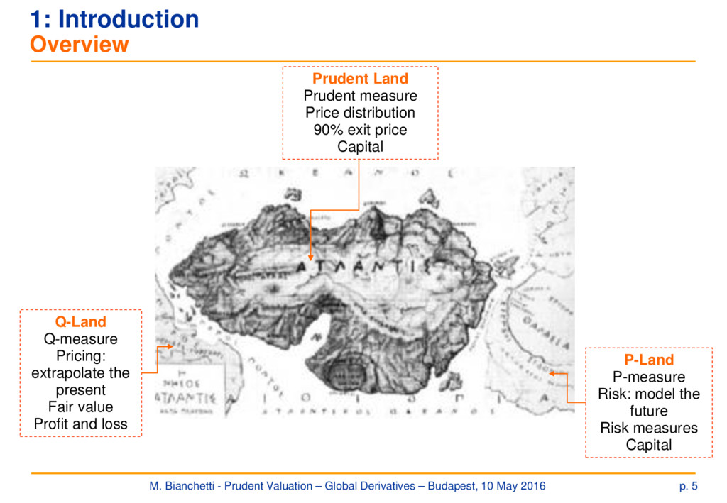
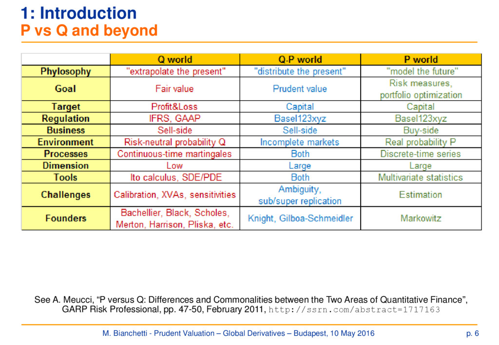
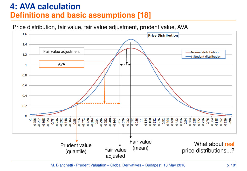
Traditionally, quantitative finance practitioners are divided into two populations: those who seek fair values, i.e. means of price distributions, and those who seek risk measures, i.e. quantiles of price distributions. Fair value people and risk people typically live in separate lands, and worship different gods: the profit and loss balance sheet, and regulatory capital, respectively.
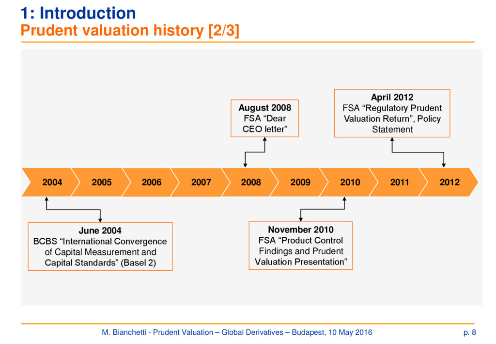
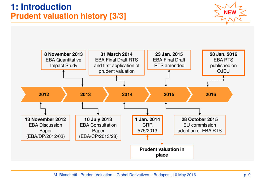
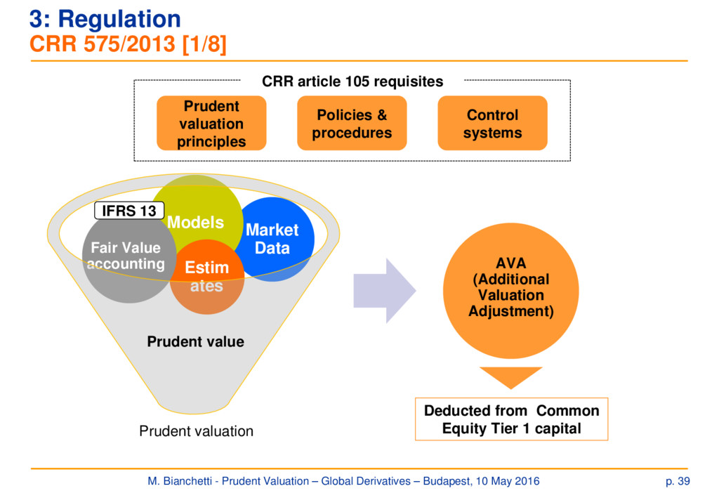
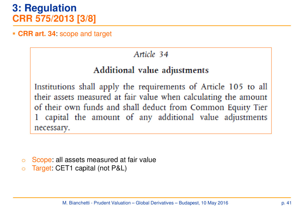
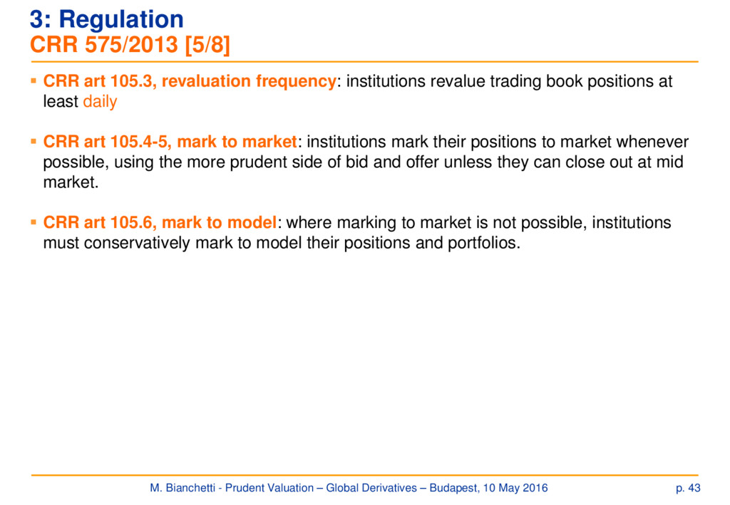
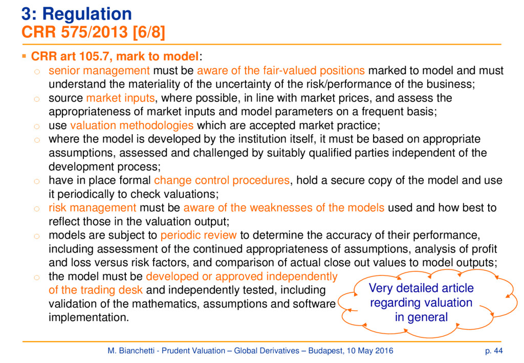
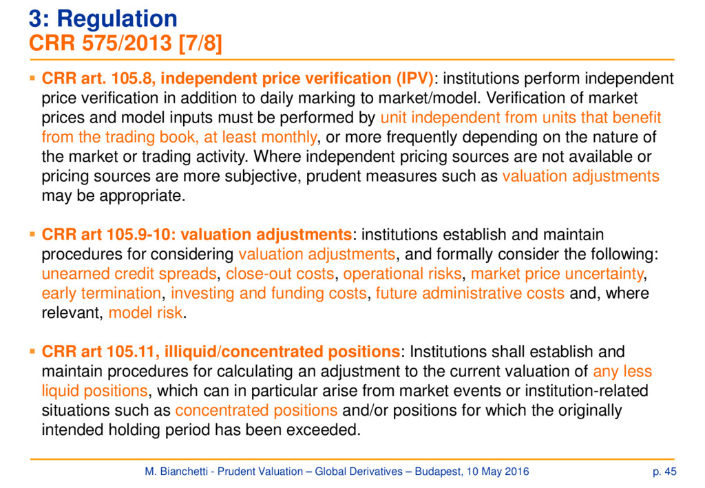
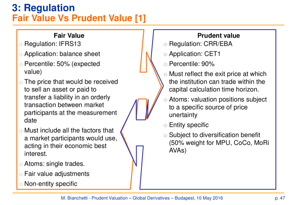
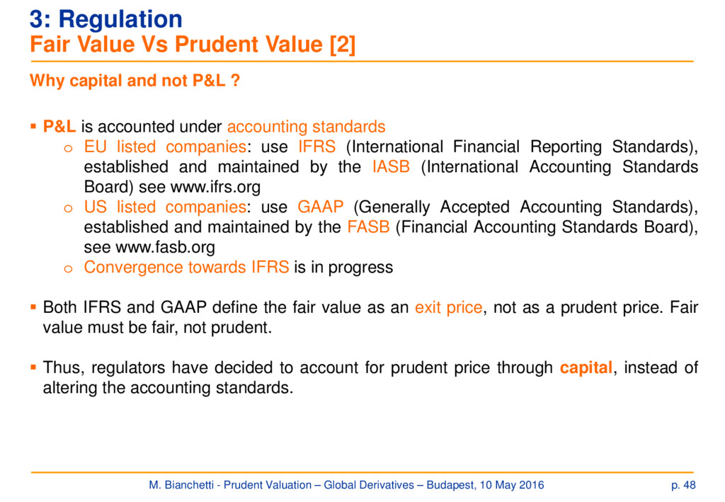
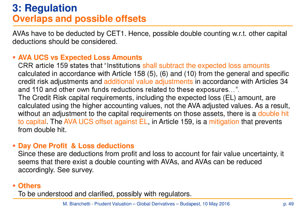
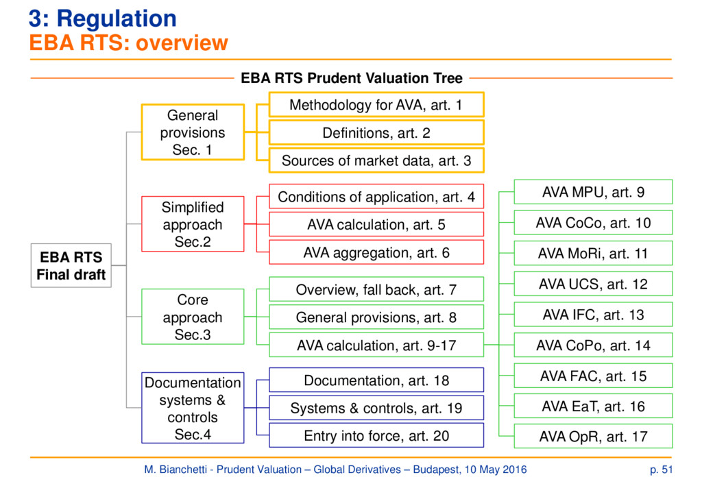
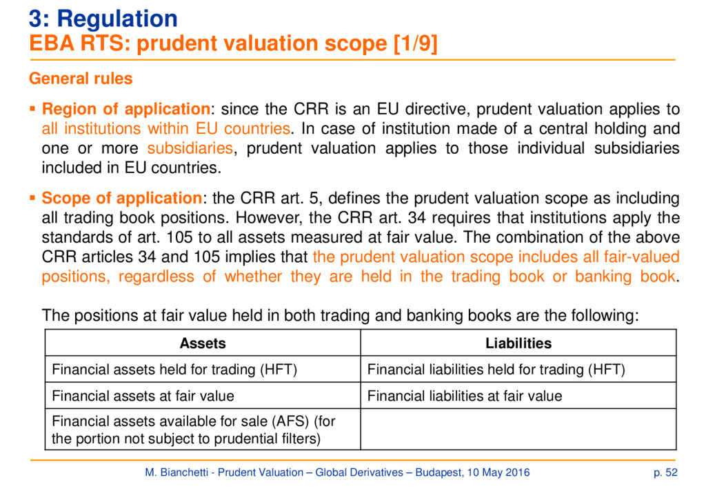
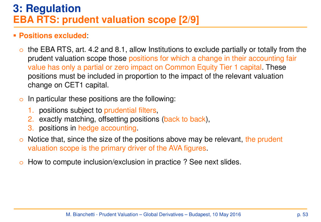
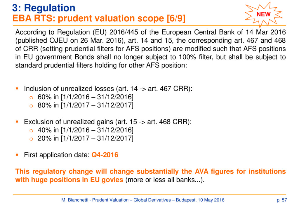
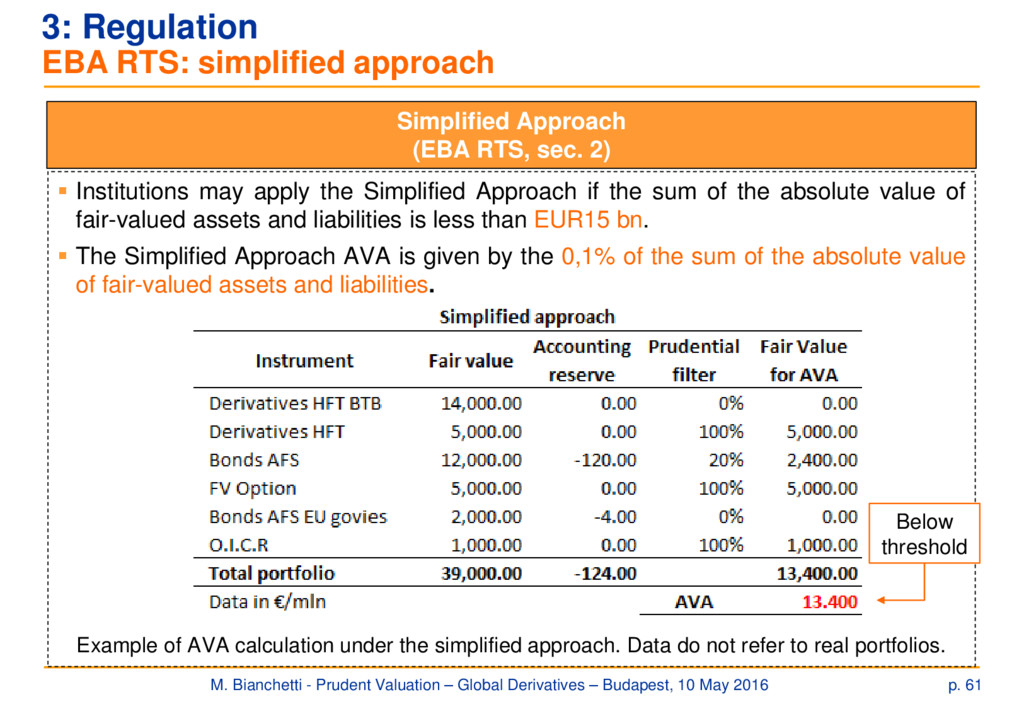
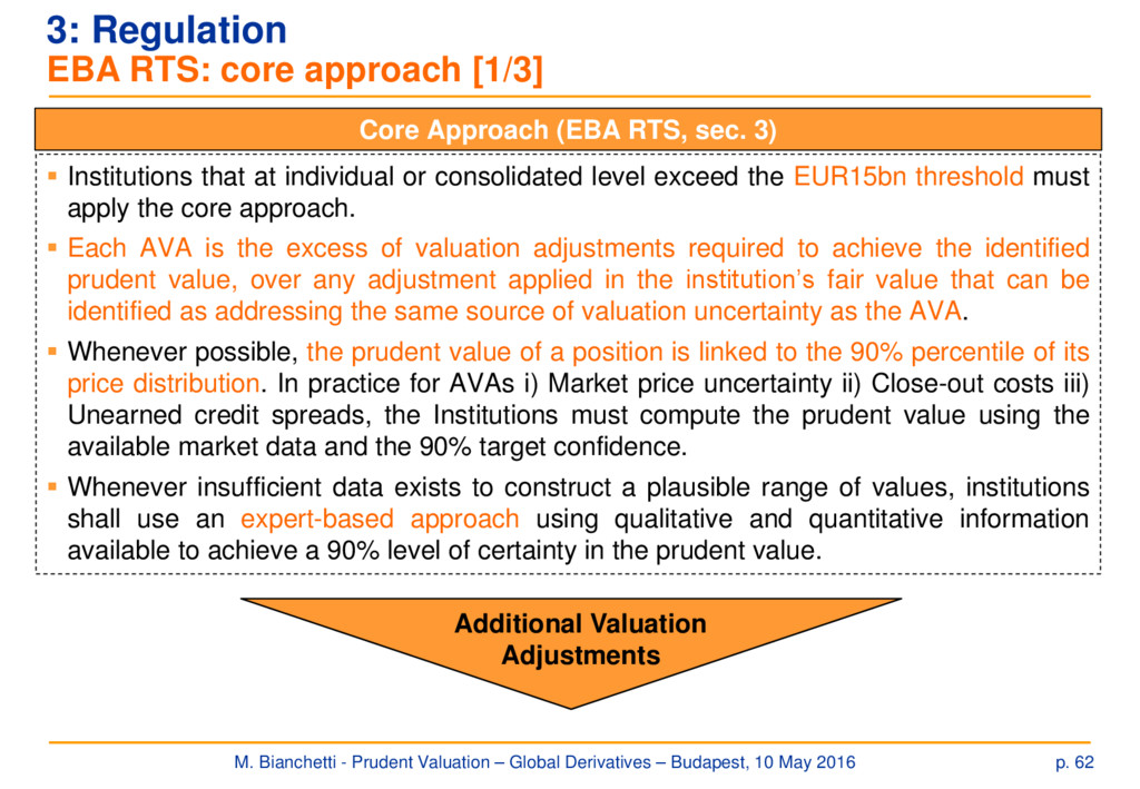
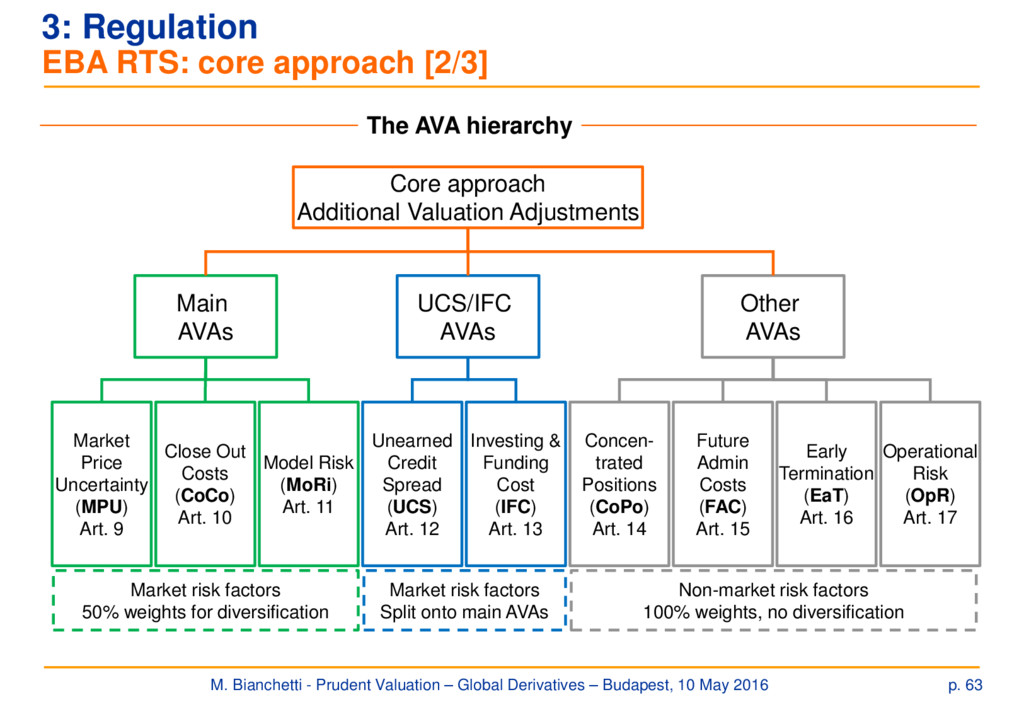
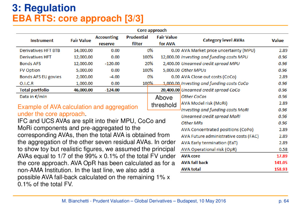
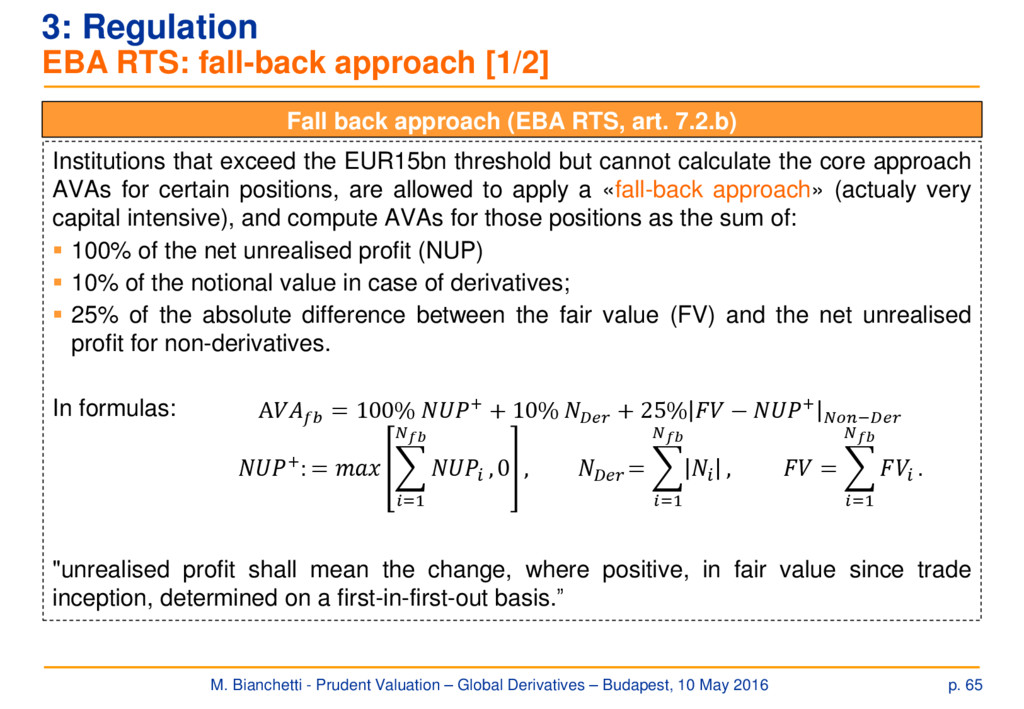
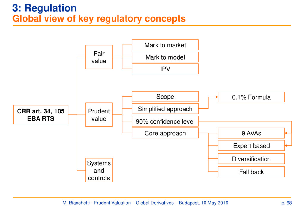
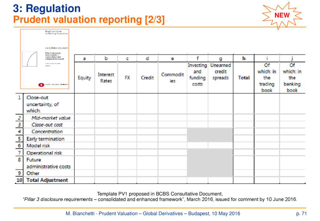
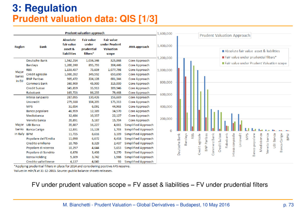
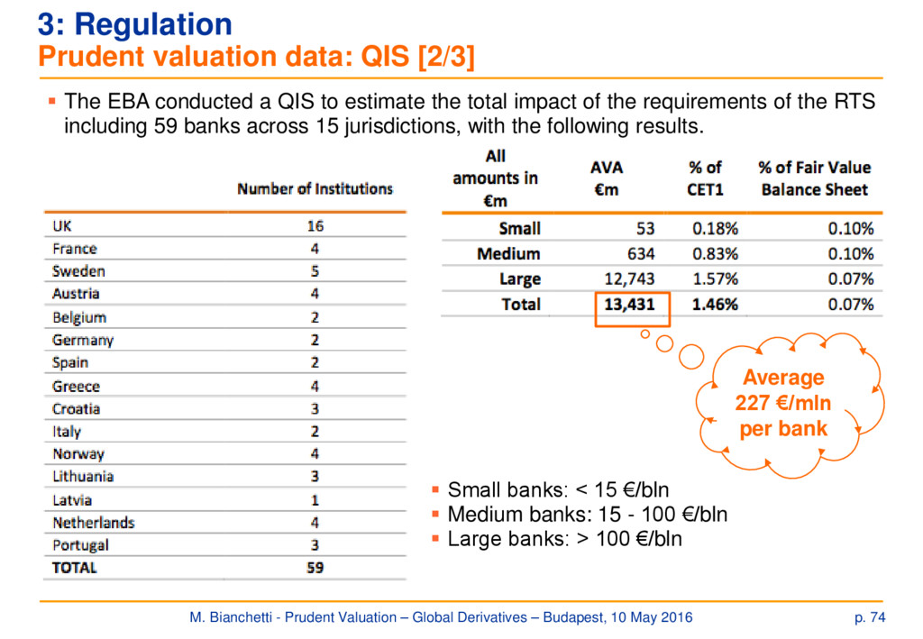
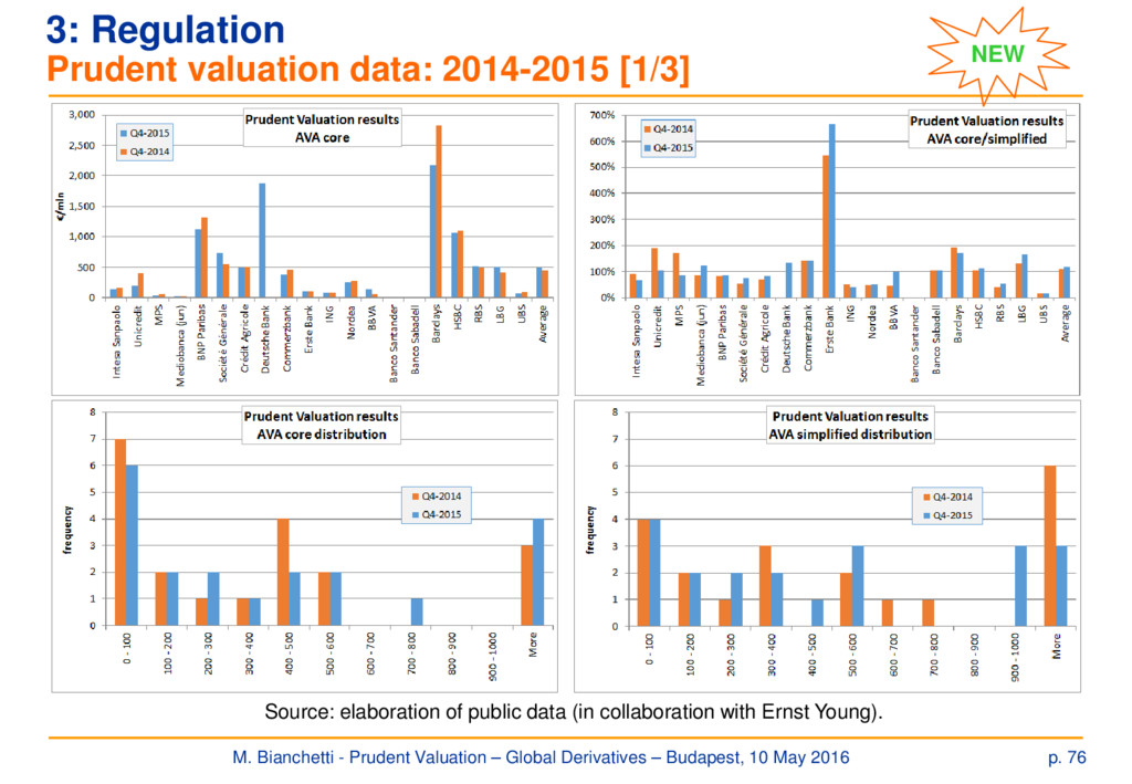
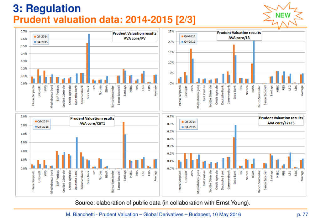
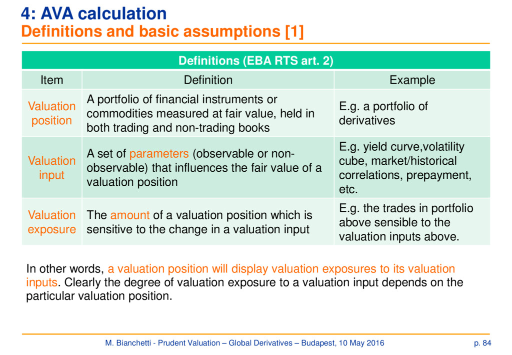
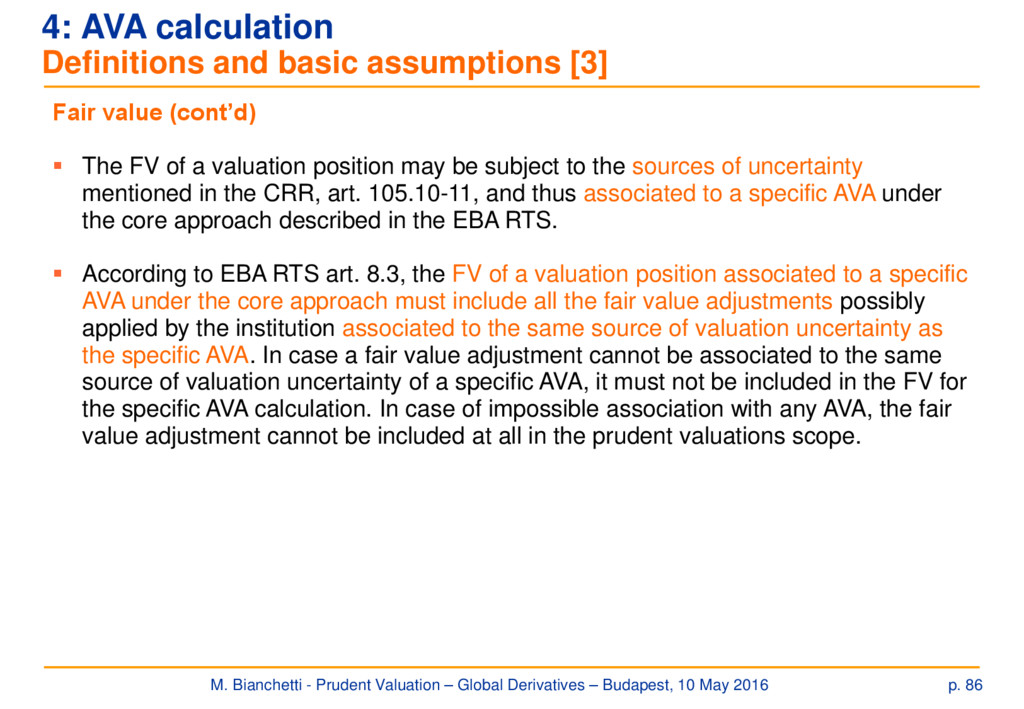
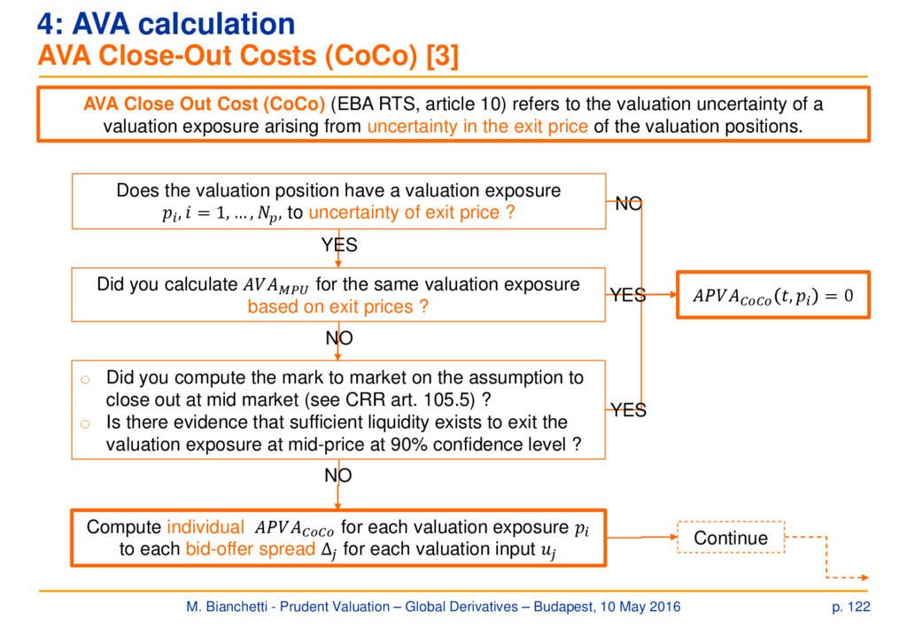
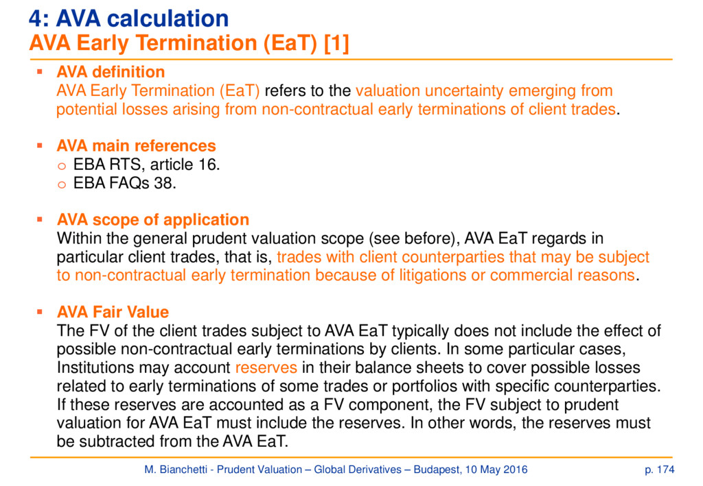
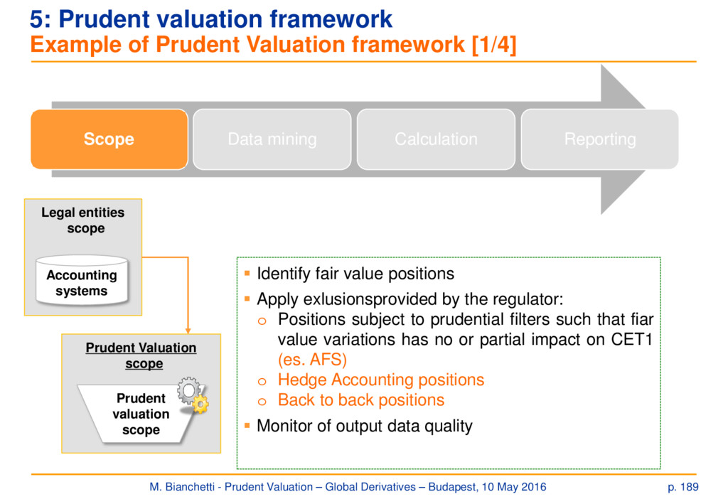
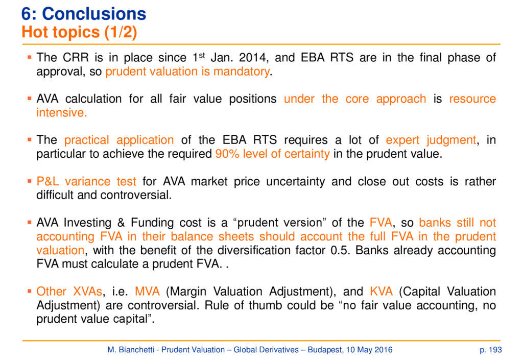
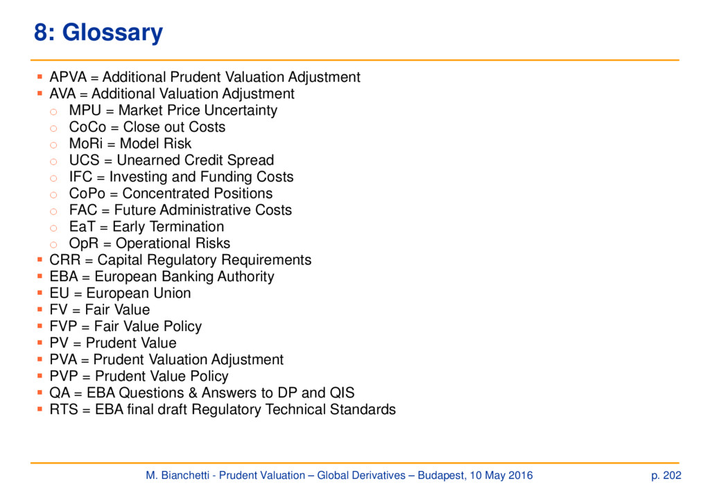
Prudent Valuation is a rather unexplored midland which has recently emerged somewhere in between the well known mainlands of Pricing and Risk Management. In fact, the Capital Requirements Regulation (CRR), requires financial institutions to apply prudent valuation to all fair value positions. The difference between the prudent value and the fair value, called Additional Valuation Adjustment (AVA), is directly deducted from the Core Equity Tier 1 (CET1) capital. The Regulatory Technical Standards (RTS) for prudent valuation proposed by the EBA have been adopted by the EU (reg. 2016/101) on 28th Jan. 2016.
The 90% confidence level required by regulators for prudent valuation links quantiles of price distributions (exit prices) to capital, thus bridging the gap between the Pricing and Risk Management mainlands, and forcing the crossbreeding of the fair value and risk populations above.
In this seminar, we will explore the Prudent Valuation land.