The Kernel Trick

The mathematics behind the kernel Trick.

Transcript

1. Seminar 1 The Kernel Trick Edgar Marca Supervisor: DSc. André M.S. Barreto Petrópolis, Rio de Janeiro - Brazil May 21st and May 28th, 2015 1 / 125
2. The plan
3. The Plan General Overview 3 / 125
4. The Plan 1.- Kernel Methods 4 / 125
5. The Plan 2.- Random Projections 5 / 125
6. The Plan 3.- Deep Learning 6 / 125
7. The Plan 4.- More about Kernels 7 / 125
8. The Plan Main Goal The main goal of these set of seminars is to have enough theoretical background to understand the following papers Julien Mairal et al., Convolutional Kernel Networks. Quoc Viet Le et al., Fastfood: Approximate Kernel Expansions in Loglinear Time. Zichao Yang et al., Deep Fried Convnets. 8 / 125
9. Greetings Part of the content of these slides was done in collaboration with my study group from the School of Mathematics at UNMSM (Universidad Nacional Mayor de San Marcos, Lima - Perú). I want to thank the members of the group for the great conversations and fun time studying Support Vector Machines at the legendary office 308. DSc. Jose R. Luyo Sanchez (UNMSM). Lic. Diego A. Benavides Vidal (Currently a Master Student at UnB). Bach. Luis E. Quispe Paredes (UNMSM). Also, I want to thank DSc. André M.S. Barreto, my supervisor, for give me the freedom to choose my topic of research. As soon as I finish with my obligatory courses at LNCC, I will start working in Reinforcement Learning. :) 9 / 125
10. Table of Contents
11. Table of Contents I Motivation R to R2 Case R2 to R3 Case Cover’s Theorem Definitions Preliminaries to Cover’s Theorem Cover’s Theorem References for Cover’s Theorem Mercer’s Theorem Theory of Bounded Linear Operators Integral Operators Preliminaries to Mercer Theorem Mercer’s Theorem References for Mercer’s Theorem Moore-Aronszajn Theorem Reproducing Kernel Hilbert Spaces 11 / 125
12. Table of Contents II Moore-Aronszajn Theorem References for Moore-Aronszajn Theorem Kernel Trick Definitions Feature Space based on Mercer’s Theorem History References 12 / 125
13. "Nothing is more practical than a good theory." — From Vapnik’s preface to The Nature of Statistical Learning Theory 13 / 125
14. Motivation
15. Motivation Motivation How we can split data that is not linear separable? How we can utilize algorithms that works for linear separable data that only depends on the inner product? 15 / 125
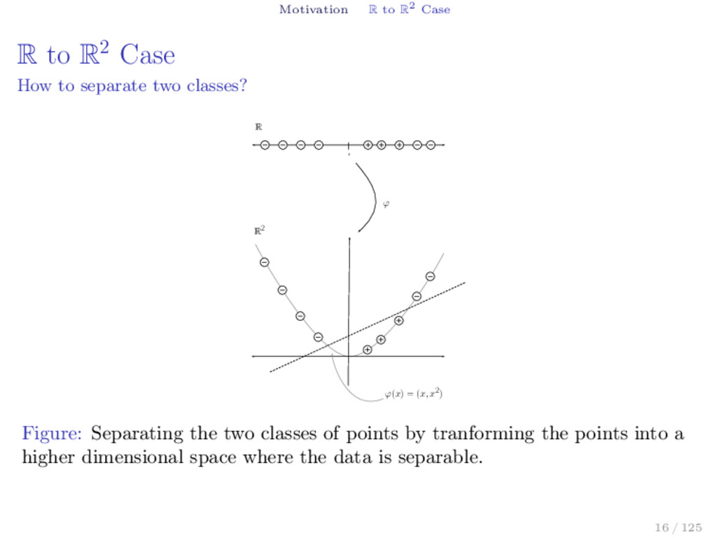
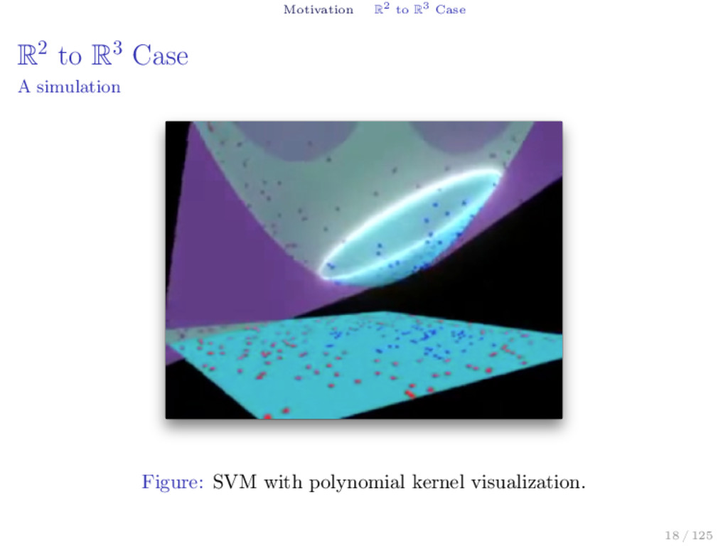
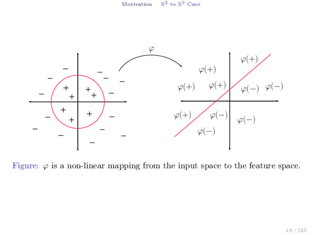
16. Motivation R to R2 Case R to R2 Case How to separate two classes? 0 R R2 ϕ(x) = (x, x 2) ϕ Figure: Separating the two classes of points by tranforming the points into a higher dimensional space where the data is separable. 16 / 125
17. Motivation R2 to R3 Case R2 to R3 Case + + + + + + + + + + + + + + + - - - - - - - - - - - - - - - - - - - - - - - - - - - - - - - - - - - - - - Figure: Data which is not linear separable. 17 / 125
18. Motivation R2 to R3 Case R2 to R3 Case A simulation Figure: SVM with polynomial kernel visualization. 18 / 125
19. Motivation R2 to R3 Case ϕ ϕ(+) ϕ(+) ϕ(+) ϕ(−) ϕ(−) ϕ(−) ϕ(−) ϕ(−) ϕ(+) ϕ(+) Figure: ϕ is a non-linear mapping from the input space to the feature space. 19 / 125
20. Cover’s Theorem
21. Cover’s Theorem Definitions During this section we will consider X a finite subset of Rd X = {x1 , x2 , . . . , xN } (1) where N a fixed natural number and xi in Rd for all 1 ≤ i ≤ N 21 / 125
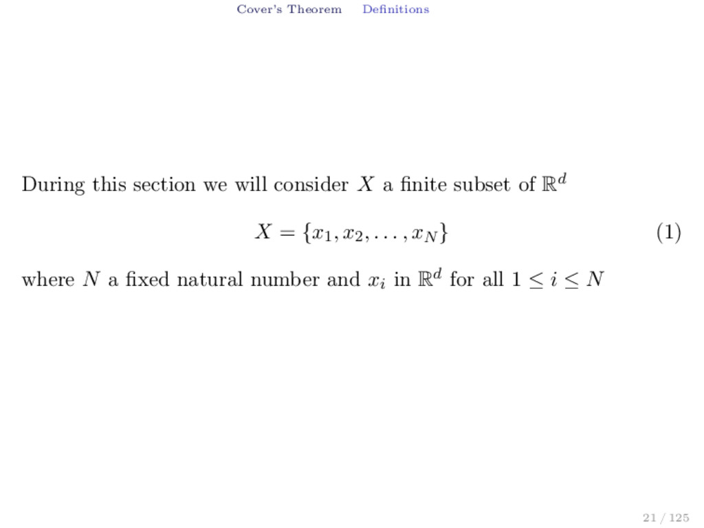
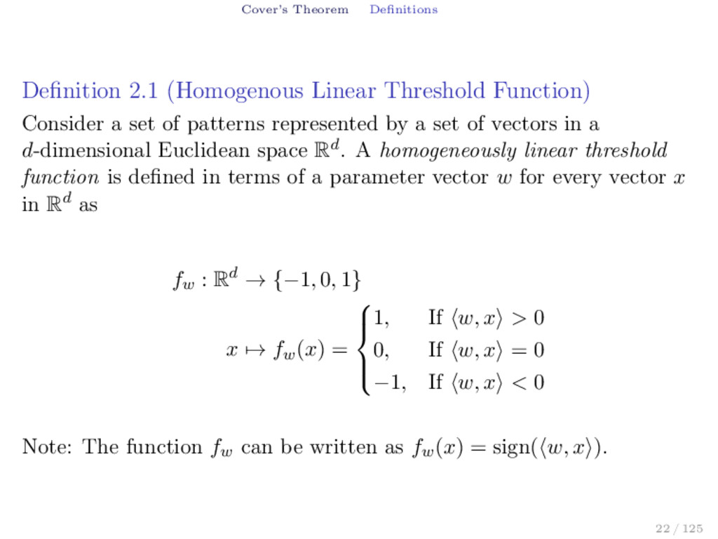
22. Cover’s Theorem Definitions Definition 2.1 (Homogenous Linear Threshold Function) Consider a set of patterns represented by a set of vectors in a d-dimensional Euclidean space Rd. A homogeneously linear threshold function is defined in terms of a parameter vector w for every vector x in Rd as fw : Rd → {−1, 0, 1} x → fw (x) =      1, If w, x > 0 0, If w, x = 0 −1, If w, x < 0 Note: The function fw can be written as fw (x) = sign( w, x ). 22 / 125
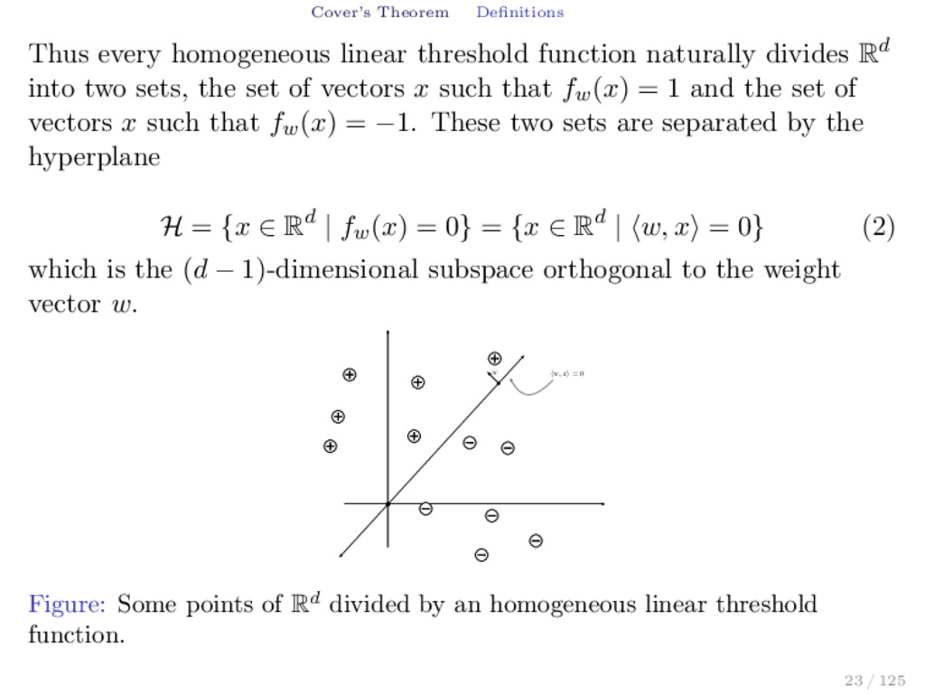
23. Cover’s Theorem Definitions Thus every homogeneous linear threshold function naturally divides Rd into two sets, the set of vectors x such that fw (x) = 1 and the set of vectors x such that fw (x) = −1. These two sets are separated by the hyperplane H = {x ∈ Rd | fw (x) = 0} = {x ∈ Rd | w, x = 0} (2) which is the (d − 1)-dimensional subspace orthogonal to the weight vector w. w w, x = 0 Figure: Some points of Rd divided by an homogeneous linear threshold function. 23 / 125
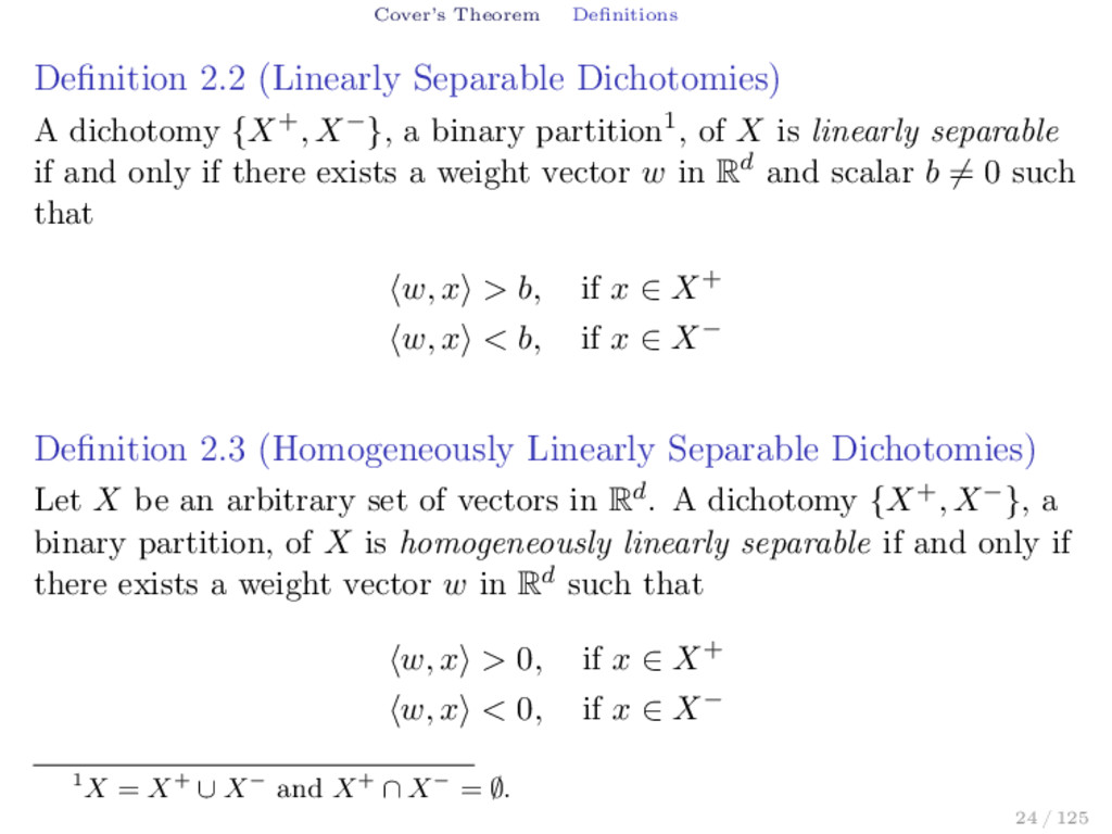
24. Cover’s Theorem Definitions Definition 2.2 (Linearly Separable Dichotomies) A dichotomy {X+, X−}, a binary partition1, of X is linearly separable if and only if there exists a weight vector w in Rd and scalar b = 0 such that w, x > b, if x ∈ X+ w, x < b, if x ∈ X− Definition 2.3 (Homogeneously Linearly Separable Dichotomies) Let X be an arbitrary set of vectors in Rd. A dichotomy {X+, X−}, a binary partition, of X is homogeneously linearly separable if and only if there exists a weight vector w in Rd such that w, x > 0, if x ∈ X+ w, x < 0, if x ∈ X− 1X = X+ ∪ X− and X+ ∩ X− = ∅. 24 / 125
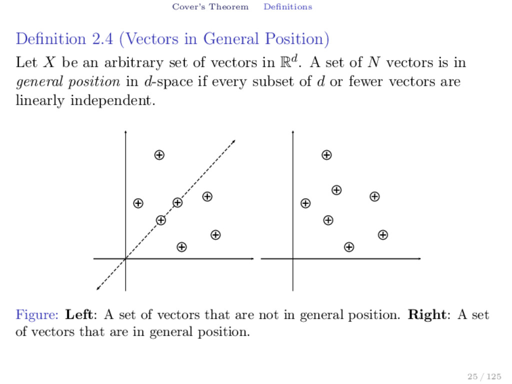
25. Cover’s Theorem Definitions Definition 2.4 (Vectors in General Position) Let X be an arbitrary set of vectors in Rd. A set of N vectors is in general position in d-space if every subset of d or fewer vectors are linearly independent. Figure: Left: A set of vectors that are not in general position. Right: A set of vectors that are in general position. 25 / 125
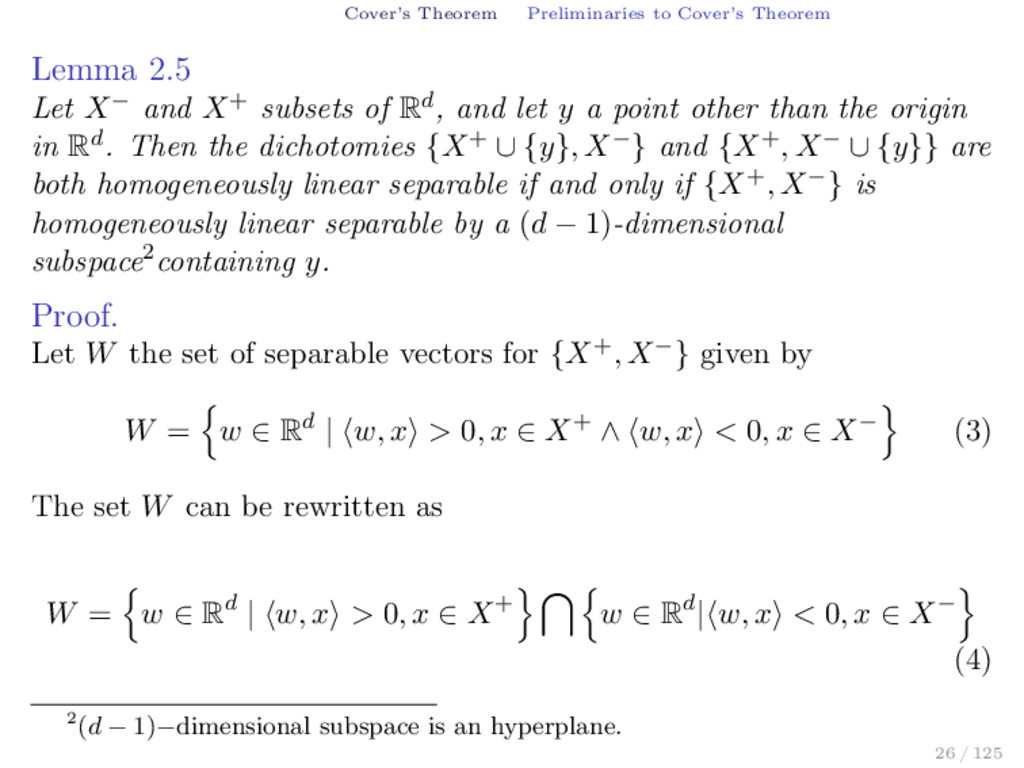
26. Cover’s Theorem Preliminaries to Cover’s Theorem Lemma 2.5 Let X− and X+ subsets of Rd, and let y a point other than the origin in Rd. Then the dichotomies {X+ ∪ {y}, X−} and {X+, X− ∪ {y}} are both homogeneously linear separable if and only if {X+, X−} is homogeneously linear separable by a (d − 1)-dimensional subspace2containing y. Proof. Let W the set of separable vectors for {X+, X−} given by W = w ∈ Rd | w, x > 0, x ∈ X+ ∧ w, x < 0, x ∈ X− (3) The set W can be rewritten as W = w ∈ Rd | w, x > 0, x ∈ X+ w ∈ Rd| w, x < 0, x ∈ X− (4) 2(d − 1)−dimensional subspace is an hyperplane. 26 / 125
27. Cover’s Theorem Preliminaries to Cover’s Theorem y w1 w2 w∗ Figure: We construct a hyperplane passing thought y which vector weight is w∗ = − w2 , y w1 + w1 , y w2. 27 / 125
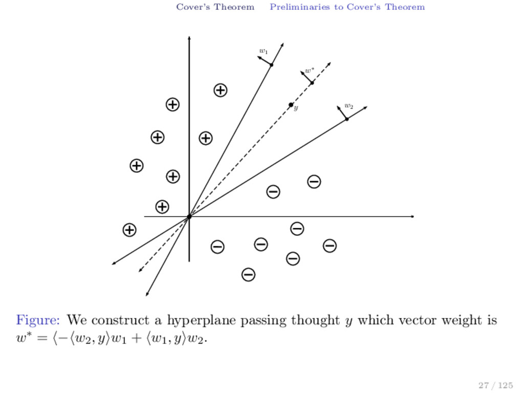
28. Cover’s Theorem Preliminaries to Cover’s Theorem The dichotomy {X+ ∪ {y}, X−} is homogeneously separable if and only if there is a vector w in W such that w, y > 0 and the dichotomy {X+, X− ∪ {y}} is homogeneously linearly separable if and only if there is a w in W such that w, y < 0. If {X+ ∪ {y}, X−} and {X+, X− ∪ {y}} are homogeneously separable by w1 and w2 respectively, then we can construct a w∗ as w∗ = − w2 , y w1 + w1 , y w2 (5) such that separates {X+, X−} by the hyperplane H = {x ∈ Rd | w∗, x = 0} passing thought y. We affirm that y belongs to H. Indeed, w∗, y = − w2 , y w1 + w1 , y w2 , y = − w2 , y w1 , y + w1 , y w2 , y = 0 28 / 125
29. Cover’s Theorem Preliminaries to Cover’s Theorem We affirm that w∗, x > 0 if x in X+. In fact, let x in X+ then w∗, x = − w2 , y w1 + w1 , y w2 , x = − w2 , y >0 w1 , x >0 + w1 , y >0 w2 , x >0 > 0 then w∗, x > 0 for all x in X+. We affirm that w∗, x < 0 if x in X−. In fact, let x in X− then w∗, x = − w2 , y w1 + w1 , y w2 , x = − w2 , y <0 w1 , x >0 + w1 , y >0 w2 , x <0 < 0 then w∗, x < 0 for all x in X−. We conclude that {X+, X−} is homogeneously separable by the vector w∗. 29 / 125
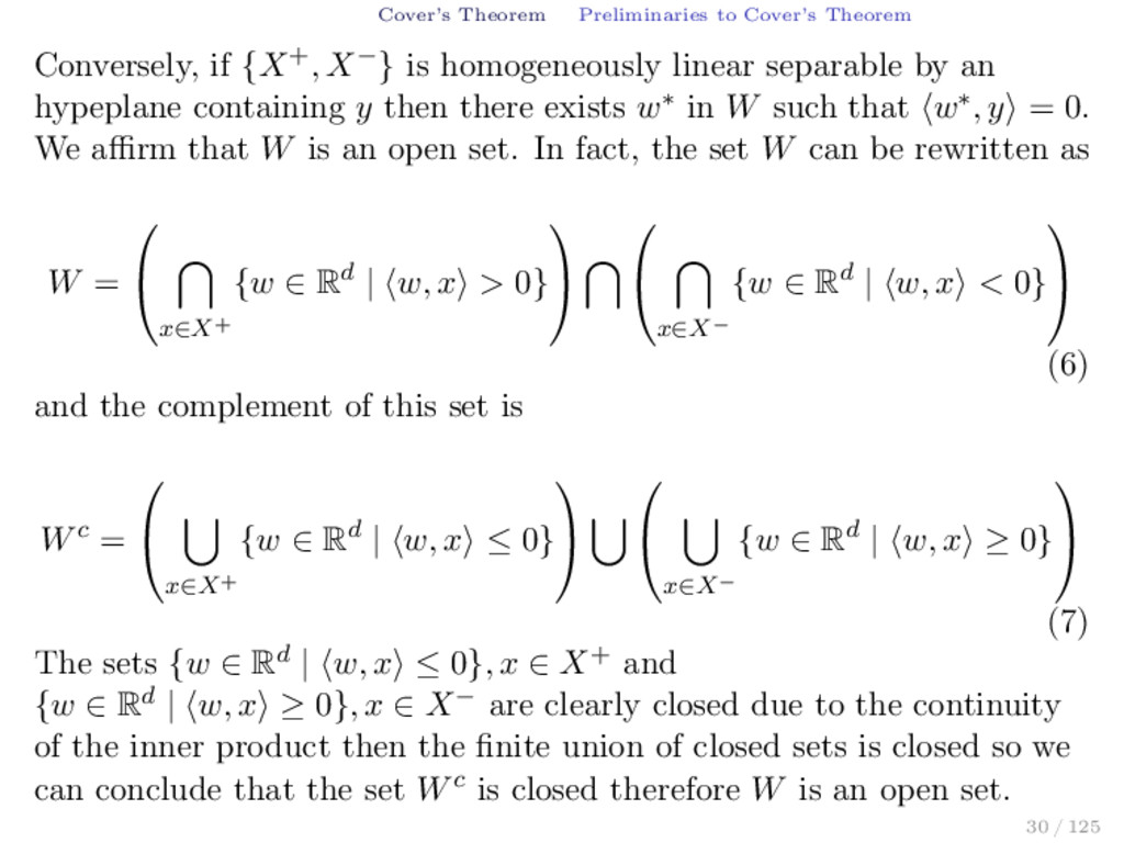
30. Cover’s Theorem Preliminaries to Cover’s Theorem Conversely, if {X+, X−} is homogeneously linear separable by an hypeplane containing y then there exists w∗ in W such that w∗, y = 0. We affirm that W is an open set. In fact, the set W can be rewritten as W =   x∈X+ {w ∈ Rd | w, x > 0}     x∈X− {w ∈ Rd | w, x < 0}   (6) and the complement of this set is Wc =   x∈X+ {w ∈ Rd | w, x ≤ 0}     x∈X− {w ∈ Rd | w, x ≥ 0}   (7) The sets {w ∈ Rd | w, x ≤ 0}, x ∈ X+ and {w ∈ Rd | w, x ≥ 0}, x ∈ X− are clearly closed due to the continuity of the inner product then the finite union of closed sets is closed so we can conclude that the set Wc is closed therefore W is an open set. 30 / 125
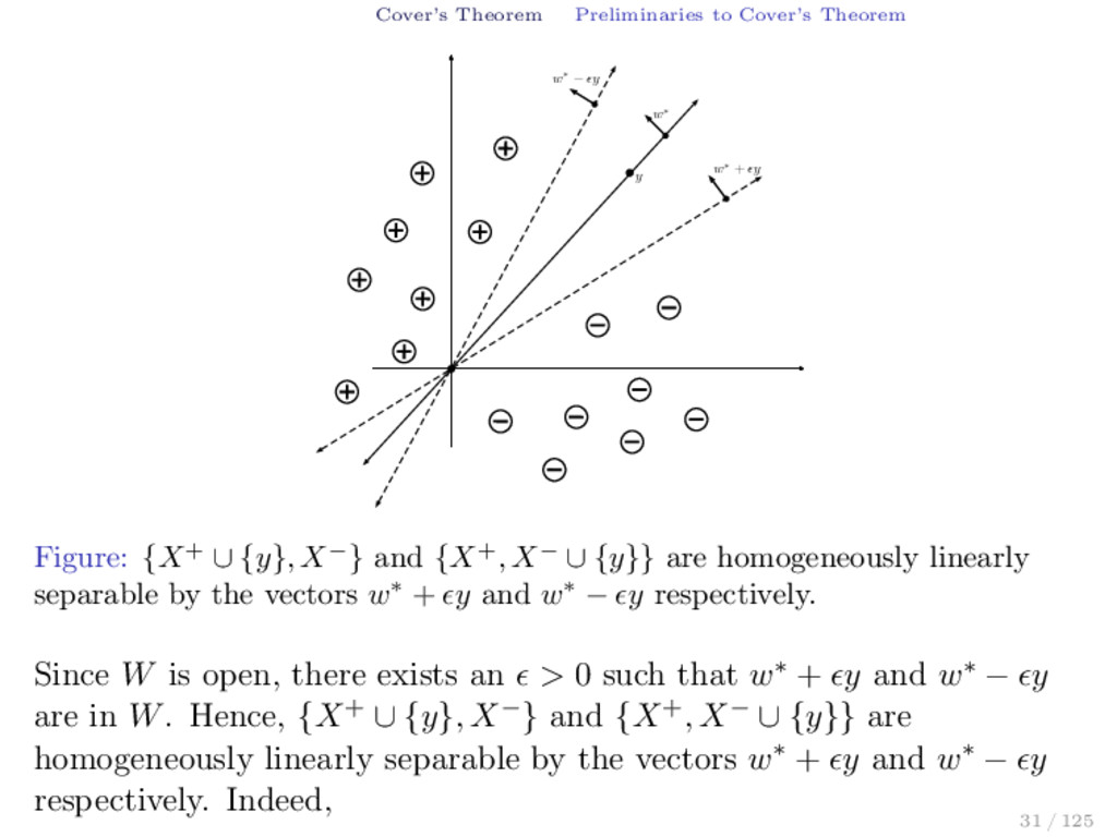
31. Cover’s Theorem Preliminaries to Cover’s Theorem y w∗ − ǫy w∗ + ǫy w∗ Figure: {X+ ∪ {y}, X−} and {X+, X− ∪ {y}} are homogeneously linearly separable by the vectors w∗ + y and w∗ − y respectively. Since W is open, there exists an > 0 such that w∗ + y and w∗ − y are in W. Hence, {X+ ∪ {y}, X−} and {X+, X− ∪ {y}} are homogeneously linearly separable by the vectors w∗ + y and w∗ − y respectively. Indeed, 31 / 125
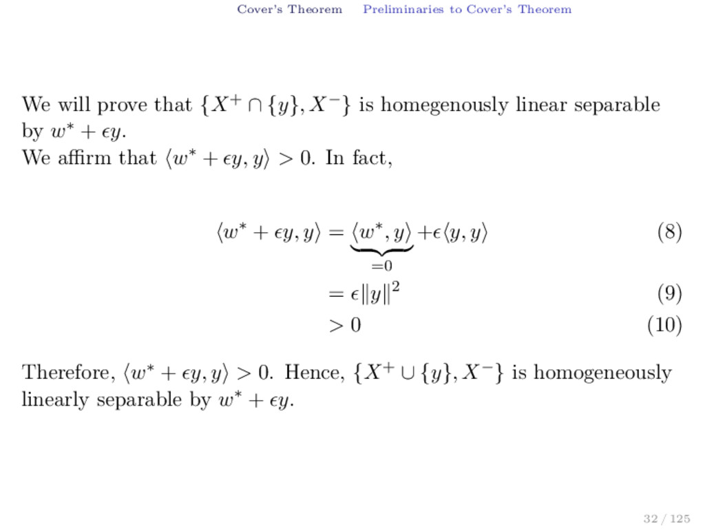
32. Cover’s Theorem Preliminaries to Cover’s Theorem We will prove that {X+ ∩ {y}, X−} is homegenously linear separable by w∗ + y. We affirm that w∗ + y, y > 0. In fact, w∗ + y, y = w∗, y =0 + y, y (8) = y 2 (9) > 0 (10) Therefore, w∗ + y, y > 0. Hence, {X+ ∪ {y}, X−} is homogeneously linearly separable by w∗ + y. 32 / 125
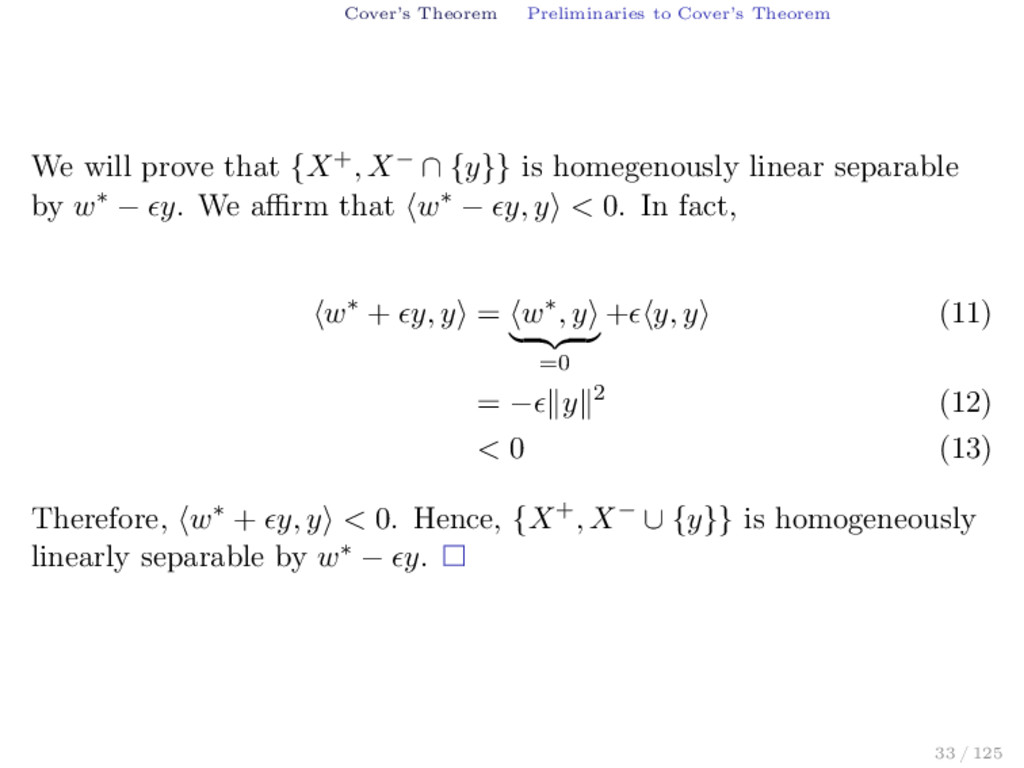
33. Cover’s Theorem Preliminaries to Cover’s Theorem We will prove that {X+, X− ∩ {y}} is homegenously linear separable by w∗ − y. We affirm that w∗ − y, y < 0. In fact, w∗ + y, y = w∗, y =0 + y, y (11) = − y 2 (12) < 0 (13) Therefore, w∗ + y, y < 0. Hence, {X+, X− ∪ {y}} is homogeneously linearly separable by w∗ − y. 33 / 125
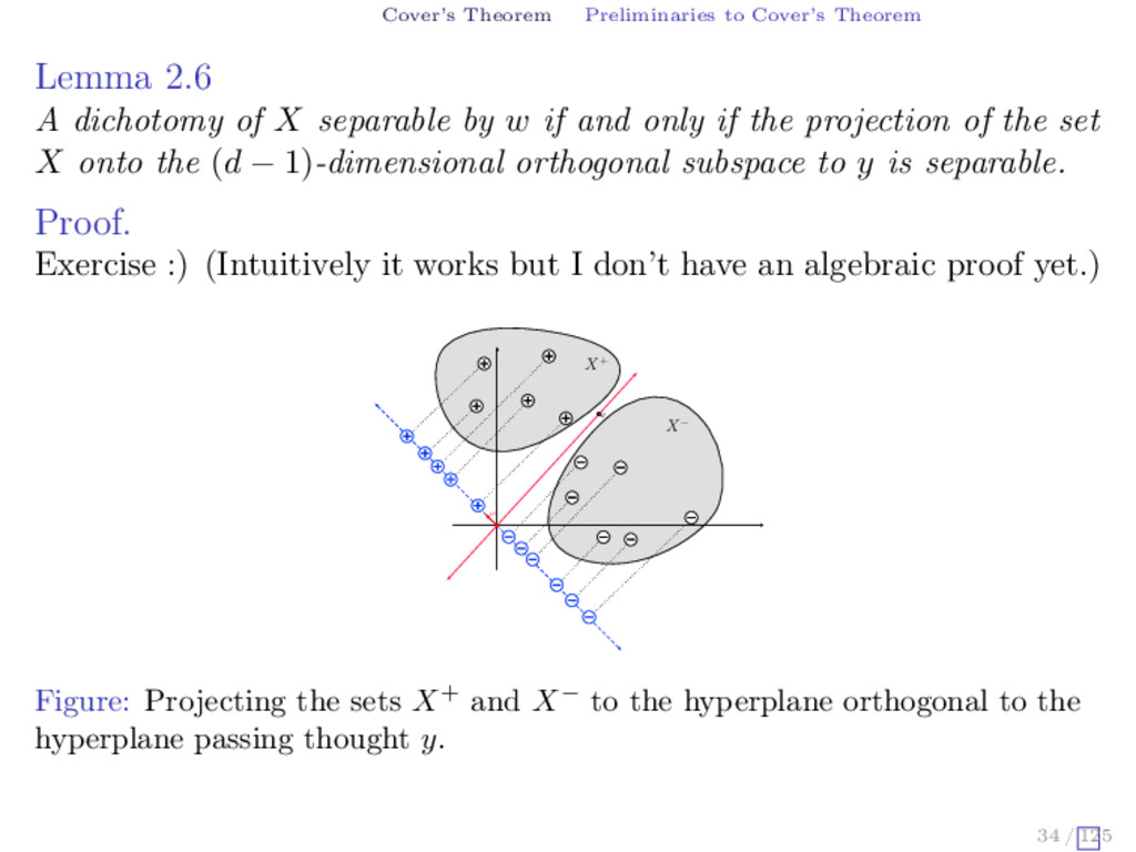
34. Cover’s Theorem Preliminaries to Cover’s Theorem Lemma 2.6 A dichotomy of X separable by w if and only if the projection of the set X onto the (d − 1)-dimensional orthogonal subspace to y is separable. Proof. Exercise :) (Intuitively it works but I don’t have an algebraic proof yet.) y w X+ X− Figure: Projecting the sets X+ and X− to the hyperplane orthogonal to the hyperplane passing thought y. 34 / 125
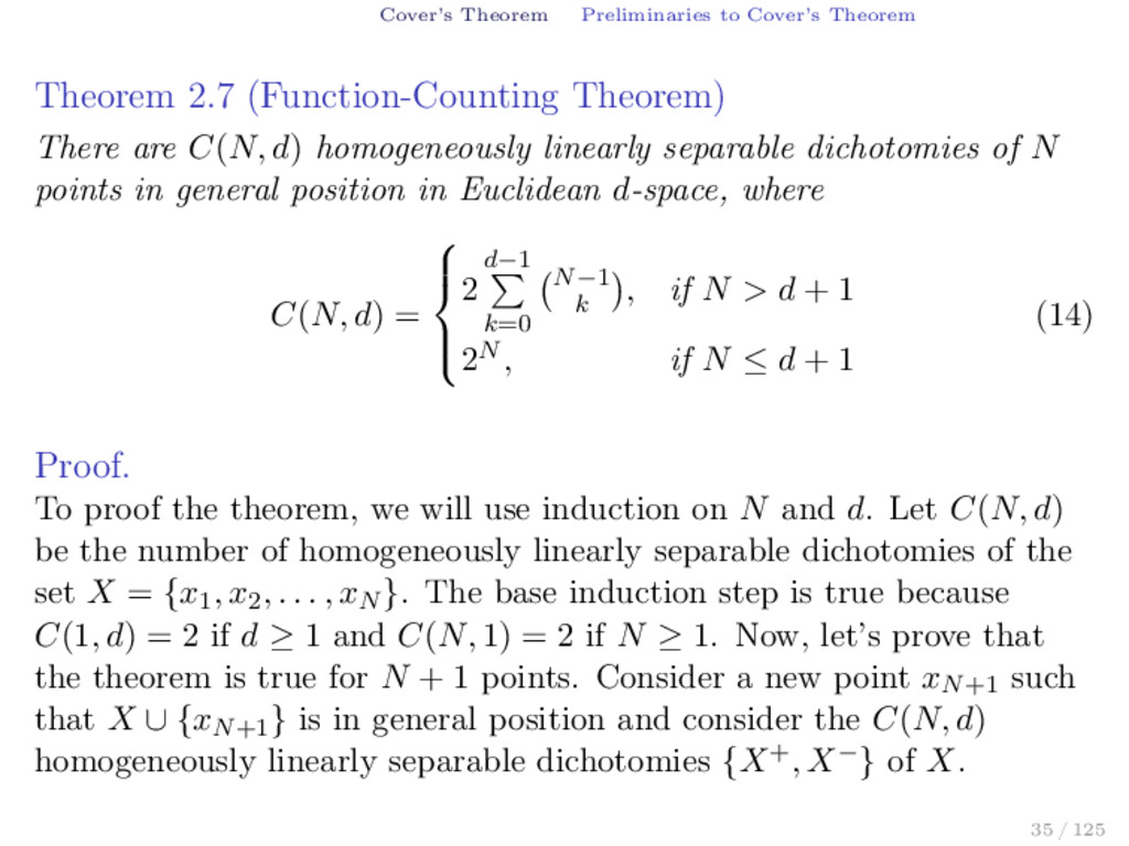
35. Cover’s Theorem Preliminaries to Cover’s Theorem Theorem 2.7 (Function-Counting Theorem) There are C(N, d) homogeneously linearly separable dichotomies of N points in general position in Euclidean d-space, where C(N, d) =      2 d−1 k=0 N−1 k , if N > d + 1 2N , if N ≤ d + 1 (14) Proof. To proof the theorem, we will use induction on N and d. Let C(N, d) be the number of homogeneously linearly separable dichotomies of the set X = {x1 , x2 , . . . , xN }. The base induction step is true because C(1, d) = 2 if d ≥ 1 and C(N, 1) = 2 if N ≥ 1. Now, let’s prove that the theorem is true for N + 1 points. Consider a new point xN+1 such that X ∪ {xN+1 } is in general position and consider the C(N, d) homogeneously linearly separable dichotomies {X+, X−} of X. 35 / 125
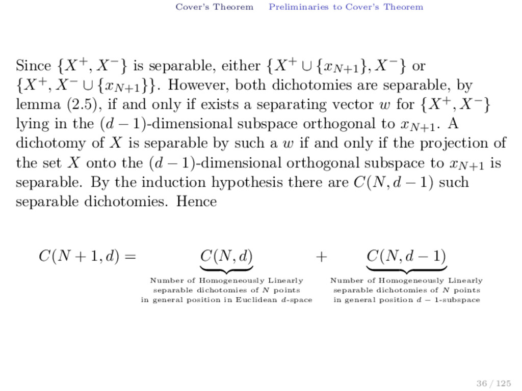
36. Cover’s Theorem Preliminaries to Cover’s Theorem Since {X+, X−} is separable, either {X+ ∪ {xN+1 }, X−} or {X+, X− ∪ {xN+1 }}. However, both dichotomies are separable, by lemma (2.5), if and only if exists a separating vector w for {X+, X−} lying in the (d − 1)-dimensional subspace orthogonal to xN+1. A dichotomy of X is separable by such a w if and only if the projection of the set X onto the (d − 1)-dimensional orthogonal subspace to xN+1 is separable. By the induction hypothesis there are C(N, d − 1) such separable dichotomies. Hence C(N + 1, d) = C(N, d) Number of Homogeneously Linearly separable dichotomies of N points in general position in Euclidean d-space + C(N, d − 1) Number of Homogeneously Linearly separable dichotomies of N points in general position d − 1-subspace 36 / 125
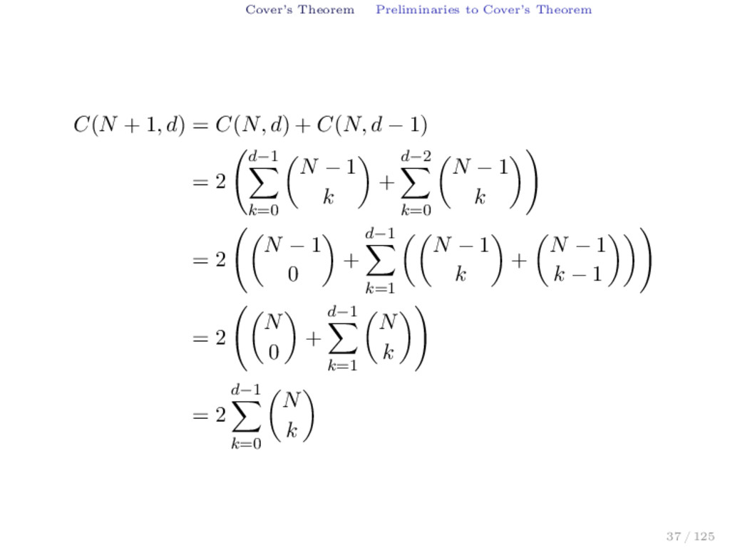
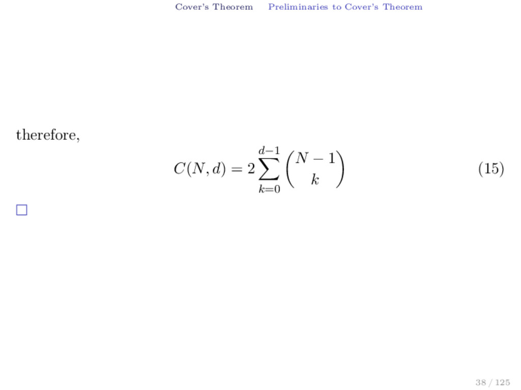
37. Cover’s Theorem Preliminaries to Cover’s Theorem C(N + 1, d) = C(N, d) + C(N, d − 1) = 2 d−1 k=0 N − 1 k + d−2 k=0 N − 1 k = 2 N − 1 0 + d−1 k=1 N − 1 k + N − 1 k − 1 = 2 N 0 + d−1 k=1 N k = 2 d−1 k=0 N k 37 / 125
38. Cover’s Theorem Preliminaries to Cover’s Theorem therefore, C(N, d) = 2 d−1 k=0 N − 1 k (15) 38 / 125
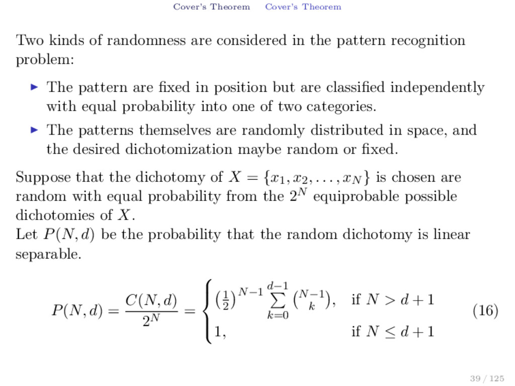
39. Cover’s Theorem Cover’s Theorem Two kinds of randomness are considered in the pattern recognition problem: The pattern are fixed in position but are classified independently with equal probability into one of two categories. The patterns themselves are randomly distributed in space, and the desired dichotomization maybe random or fixed. Suppose that the dichotomy of X = {x1 , x2 , . . . , xN } is chosen are random with equal probability from the 2N equiprobable possible dichotomies of X. Let P(N, d) be the probability that the random dichotomy is linear separable. P(N, d) = C(N, d) 2N =      1 2 N−1 d−1 k=0 N−1 k , if N > d + 1 1, if N ≤ d + 1 (16) 39 / 125
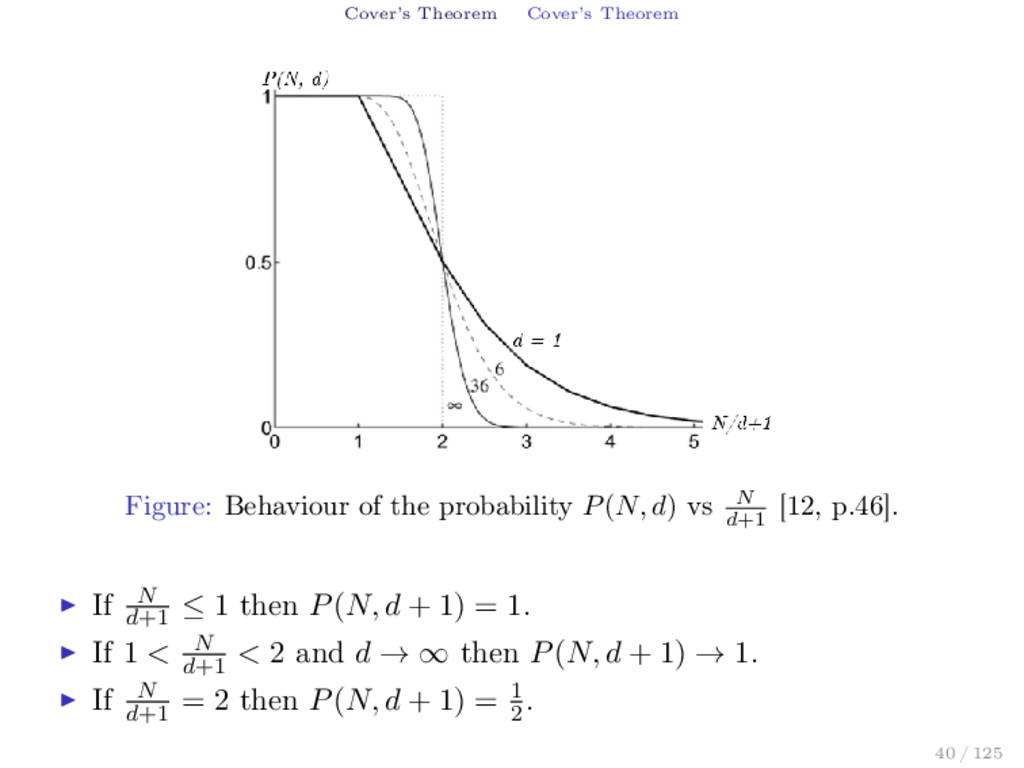
40. Cover’s Theorem Cover’s Theorem Figure: Behaviour of the probability P(N, d) vs N d+1 [12, p.46]. If N d+1 ≤ 1 then P(N, d + 1) = 1. If 1 < N d+1 < 2 and d → ∞ then P(N, d + 1) → 1. If N d+1 = 2 then P(N, d + 1) = 1 2 . 40 / 125
41. Cover’s Theorem Cover’s Theorem Theorem 2.8 (Cover’s Theorem) A complex pattern classification problem cast in a high-dimensional space nonlinearly, is more likely to be linearly separable than in a low-dimensional space. 41 / 125
42. References for Cover’s Theorem References for Cover’s Theorem Main Source: [7] Thomas Cover. “Geometrical and Statistical properties of systems of linear inequalities with applications in pattern recognition”. In: IEEE Transactions on Electronic Computer (), pp. 326–334. Minor Sources: [12] Ke-Lin Du and M. N. S. Swamy. Neural Networks and Statistical Learning. Springer Science & Business Media, 2013. [19] Simon Haykin. Neural Networks and Learning Machines. Third Edition. Pearson Prentice Hall, 2009. [39] Bernhard Schlköpf and Alexander Smola. Learning with Kernels: Support Vector Machines, Regularization, Optimization, and Beyond. The MIT Press, 2001. [49] Sergios Theodoridis. Machine Learning: A Bayesian and Optimization Perspective. Academic Press, 2015. 42 / 125
43. Mercer’s Theorem
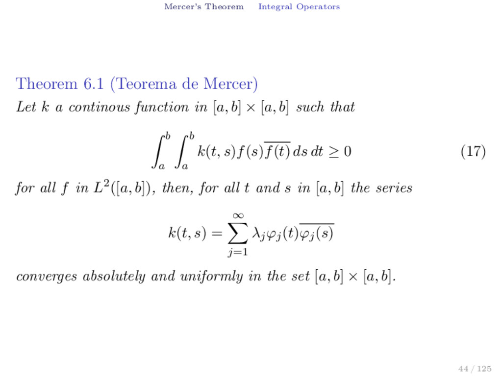
44. Mercer’s Theorem Integral Operators Theorem 6.1 (Teorema de Mercer) Let k a continous function in [a, b] × [a, b] such that b a b a k(t, s)f(s)f(t) ds dt ≥ 0 (17) for all f in L2([a, b]), then, for all t and s in [a, b] the series k(t, s) = ∞ j=1 λj ϕj (t)ϕj (s) converges absolutely and uniformly in the set [a, b] × [a, b]. 44 / 125
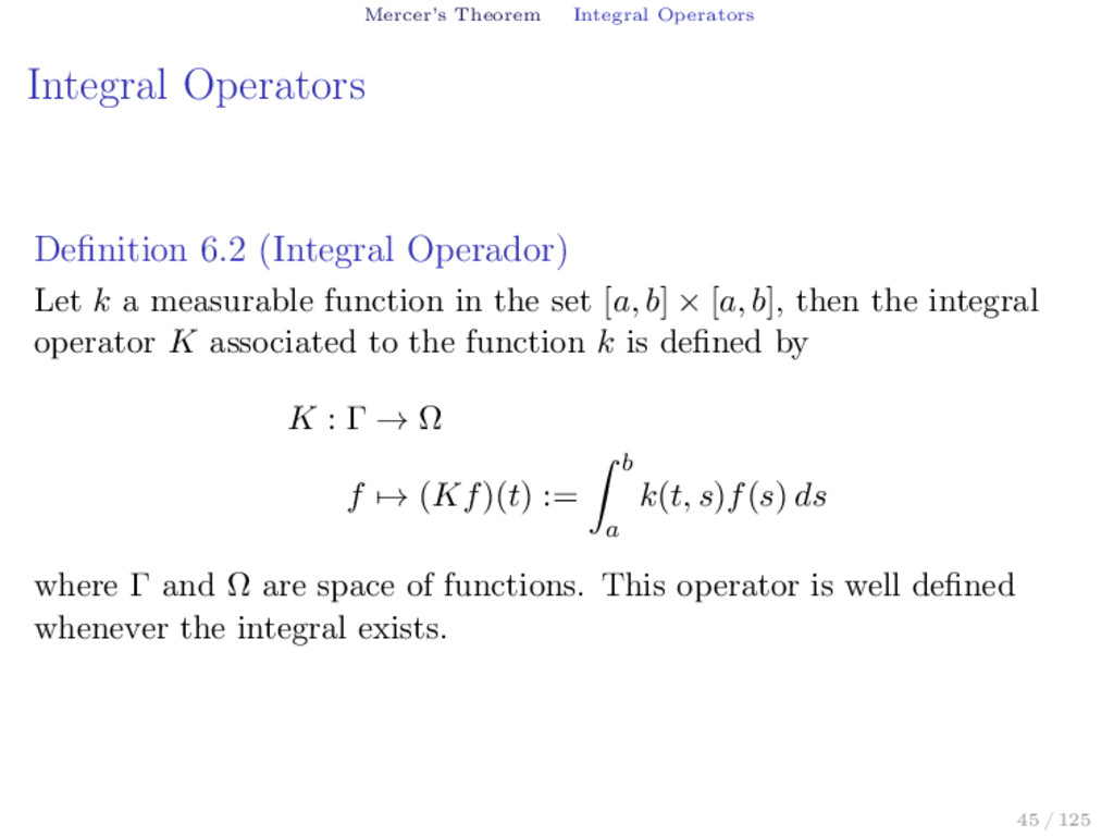
45. Mercer’s Theorem Integral Operators Integral Operators Definition 6.2 (Integral Operador) Let k a measurable function in the set [a, b] × [a, b], then the integral operator K associated to the function k is defined by K : Γ → Ω f → (Kf)(t) := b a k(t, s)f(s) ds where Γ and Ω are space of functions. This operator is well defined whenever the integral exists. 45 / 125
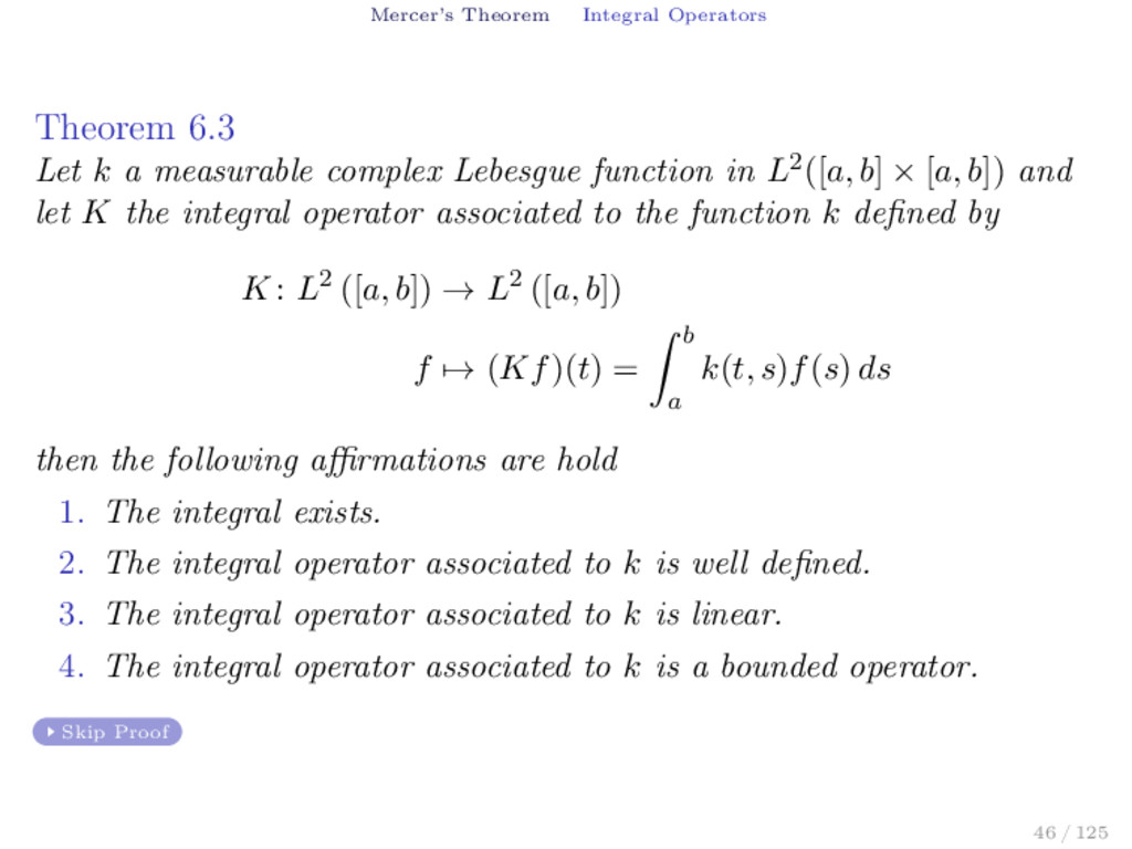
46. Mercer’s Theorem Integral Operators Theorem 6.3 Let k a measurable complex Lebesgue function in L2([a, b] × [a, b]) and let K the integral operator associated to the function k defined by K : L2 ([a, b]) → L2 ([a, b]) f → (Kf)(t) = b a k(t, s)f(s) ds then the following affirmations are hold 1. The integral exists. 2. The integral operator associated to k is well defined. 3. The integral operator associated to k is linear. 4. The integral operator associated to k is a bounded operator. Skip Proof 46 / 125
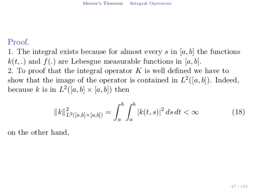
47. Mercer’s Theorem Integral Operators Proof. 1. The integral exists because for almost every s in [a, b] the functions k(t, .) and f(.) are Lebesgue measurable functions in [a, b]. 2. To proof that the integral operator K is well defined we have to show that the image of the operator is contained in L2([a, b]). Indeed, because k is in L2([a, b] × [a, b]) then k 2 L2([a,b]×[a,b]) = b a b a |k(t, s)|2 ds dt < ∞ (18) on the other hand, 47 / 125
48. Mercer’s Theorem Integral Operators Proof. Kf 2 L2([a,b]) = Kf, Kf L2([a,b]) = b a (Kf)(t)(Kf)(t) dt = b a b a k(t, s)f(s) ds b a k(t, s)f(s) ds dt = b a b a k(t, s)f(s) ds 2 dt ≤ b a b a |k(t, s)f(s)| ds 2 dt ≤ b a b a |k(t, s)|2 ds b a |f(s)|2 ds dt (D. C-S) 48 / 125
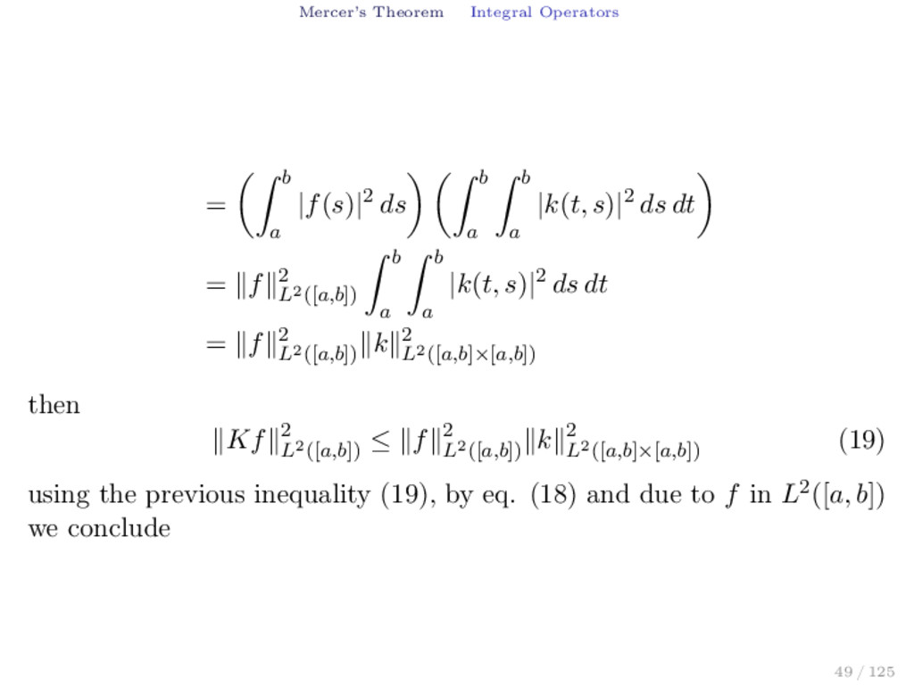
49. Mercer’s Theorem Integral Operators = b a |f(s)|2 ds b a b a |k(t, s)|2 ds dt = f 2 L2([a,b]) b a b a |k(t, s)|2 ds dt = f 2 L2([a,b]) k 2 L2([a,b]×[a,b]) then Kf 2 L2([a,b]) ≤ f 2 L2([a,b]) k 2 L2([a,b]×[a,b]) (19) using the previous inequality (19), by eq. (18) and due to f in L2([a, b]) we conclude 49 / 125
50. Mercer’s Theorem Integral Operators Kf 2 L2([a,b]) ≤ f 2 L2([a,b]) k 2 L2([a,b]×[a,b]) < ∞ (20) therefore, the functions Kf is in L2([a, b]) and we can conclude that the integral operator K is well defined. 3. Let α, β in R an f, g in L2([a, b]) then K(αf + βg) = b a [k(t, s)(αf(s) + βg(s))]ds = α b a k(t, s)f(s)ds + β b a k(t, s)g(s)ds = αK(f) + βK(g) therefore the integral operator K is a linear operator. 50 / 125
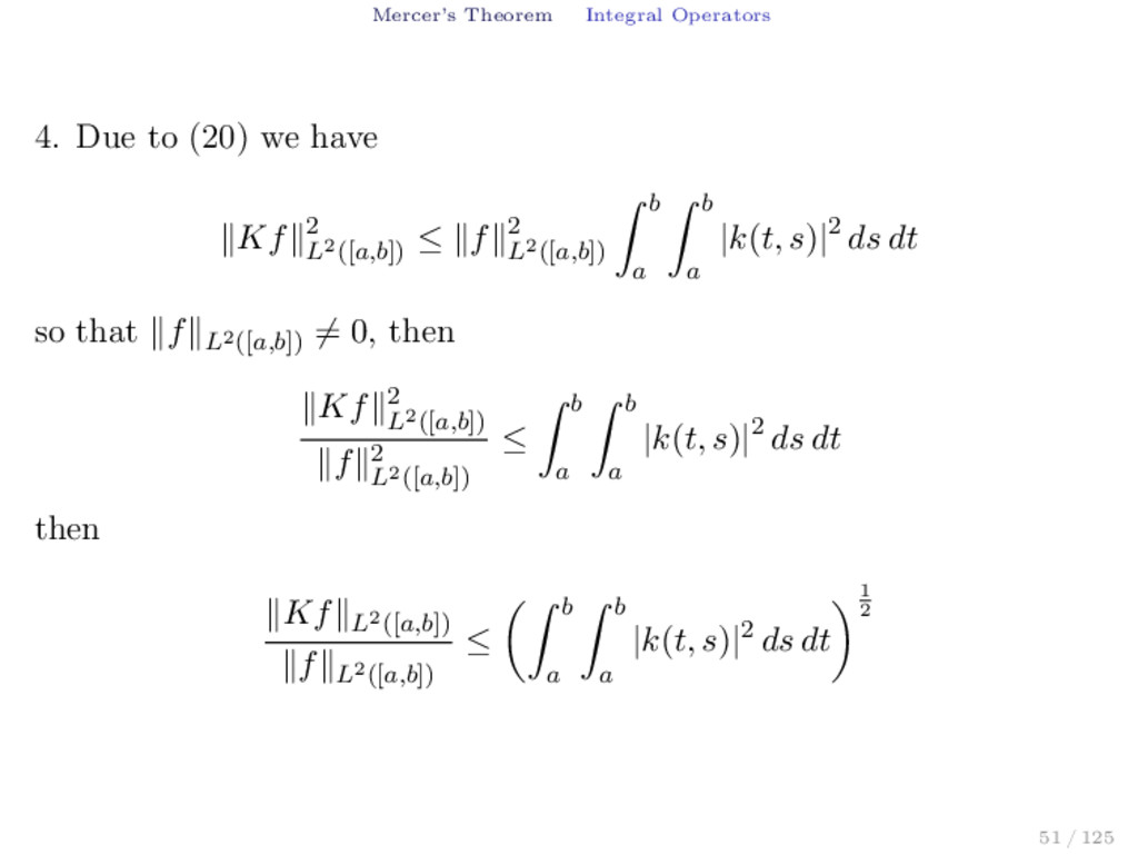
51. Mercer’s Theorem Integral Operators 4. Due to (20) we have Kf 2 L2([a,b]) ≤ f 2 L2([a,b]) b a b a |k(t, s)|2 ds dt so that f L2([a,b]) = 0, then Kf 2 L2([a,b]) f 2 L2([a,b]) ≤ b a b a |k(t, s)|2 ds dt then Kf L2([a,b]) f L2([a,b]) ≤ b a b a |k(t, s)|2 ds dt 1 2 51 / 125
52. Mercer’s Theorem Integral Operators K = sup f L2([a,b]) =0 Kf L2([a,b]) f L2([a,b]) ≤ b a b a |k(t, s)|2 ds dt 1 2 = k L2([a,b]×[a,b]) < ∞ in the last inequality using the equation (18) we can conclude that K < ∞ so K is a bounded operator. 52 / 125
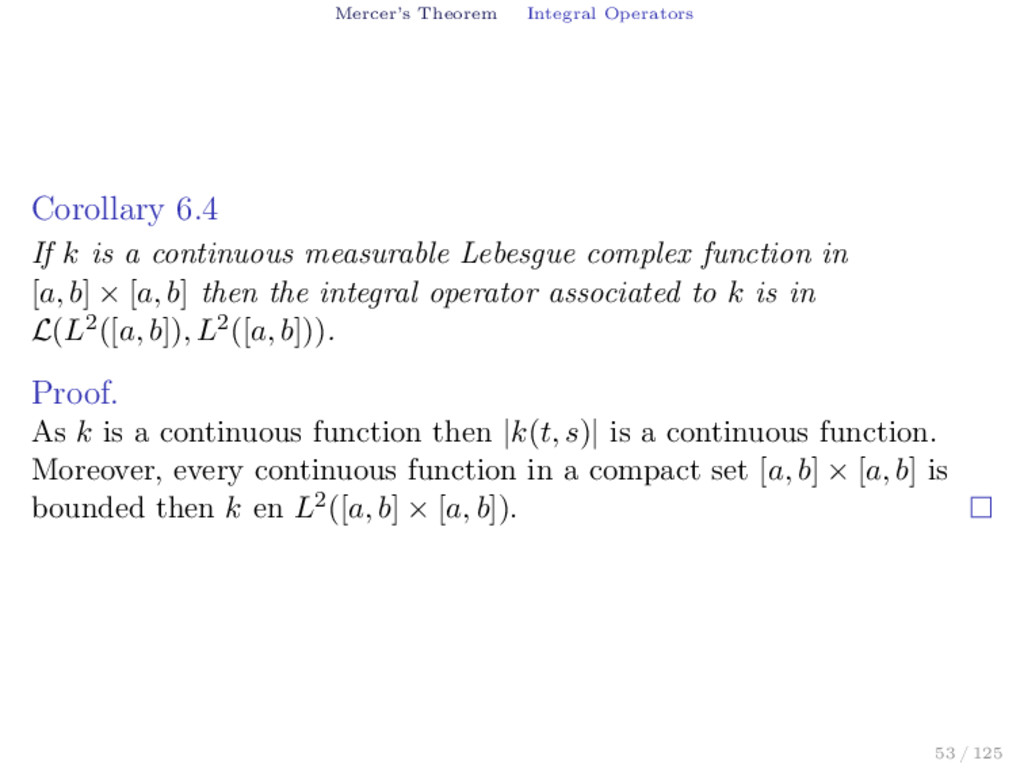
53. Mercer’s Theorem Integral Operators Corollary 6.4 If k is a continuous measurable Lebesgue complex function in [a, b] × [a, b] then the integral operator associated to k is in L(L2([a, b]), L2([a, b])). Proof. As k is a continuous function then |k(t, s)| is a continuous function. Moreover, every continuous function in a compact set [a, b] × [a, b] is bounded then k en L2([a, b] × [a, b]). 53 / 125
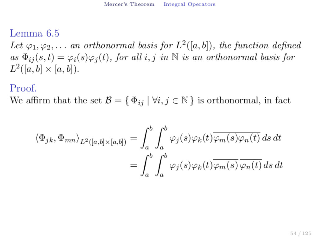
54. Mercer’s Theorem Integral Operators Lemma 6.5 Let ϕ1 , ϕ2 , . . . an orthonormal basis for L2([a, b]), the function defined as Φij (s, t) = ϕi (s)ϕj (t), for all i, j in N is an orthonormal basis for L2([a, b] × [a, b]). Proof. We affirm that the set B = { Φij | ∀i, j ∈ N } is orthonormal, in fact Φjk , Φmn L2([a,b]×[a,b]) = b a b a ϕj (s)ϕk (t)ϕm (s)ϕn (t) ds dt = b a b a ϕj (s)ϕk (t)ϕm (s) ϕn (t) ds dt 54 / 125
55. Mercer’s Theorem Integral Operators Φjk , Φmn L2([a,b]×[a,b]) = b a b a ϕj (s)ϕk (t)ϕm (s)ϕn (t) ds dt = b a b a ϕj (s)ϕk (t)ϕm (s) ϕn (t) ds dt = b a ϕj (s)ϕm (s) ds b a ϕk (t)ϕn (t) dt (T. Fubini) = δjm δkn where δjm δkn = 1, if j = m ∧ k = n 0, in other case (21) therefore B is an orthonormal set. 55 / 125
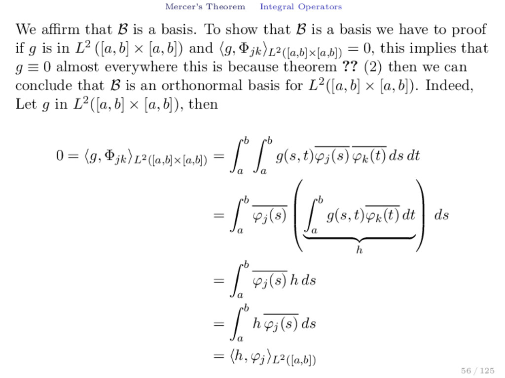
56. Mercer’s Theorem Integral Operators We affirm that B is a basis. To show that B is a basis we have to proof if g is in L2 ([a, b] × [a, b]) and g, Φjk L2([a,b]×[a,b]) = 0, this implies that g ≡ 0 almost everywhere this is because theorem ?? (2) then we can conclude that B is an orthonormal basis for L2([a, b] × [a, b]). Indeed, Let g in L2([a, b] × [a, b]), then 0 = g, Φjk L2([a,b]×[a,b]) = b a b a g(s, t)ϕj (s) ϕk (t) ds dt = b a ϕj (s)     b a g(s, t)ϕk (t) dt h     ds = b a ϕj (s) h ds = b a h ϕj (s) ds = h, ϕj L2([a,b]) 56 / 125
57. Mercer’s Theorem Integral Operators then h, ϕj L2([a,b]) = 0 (22) where the function h is h(s) = b a g(s, t)ϕk (t) dt the function h can be written in the following form h(s) = g(s, .), ϕk L2([a,b]) , ∀k = 1, 2, . . . (23) as the function h is orthonormal to every function ϕj this implies that h ≡ 0 in almost every point s in [a, b] (theorem ?? (2)). By the equation (23) and h ≡ 0 we can conclude that there is a set Ω which measure is zero such that for all s which is not in Ω the function g(s, .) is orthogonal to ϕk for all k = 1, 2, . . . therefore g(s, t) = 0 for all t and each s which doesn’t belongs to Ω (theorem ?? (2)). Therefore 57 / 125
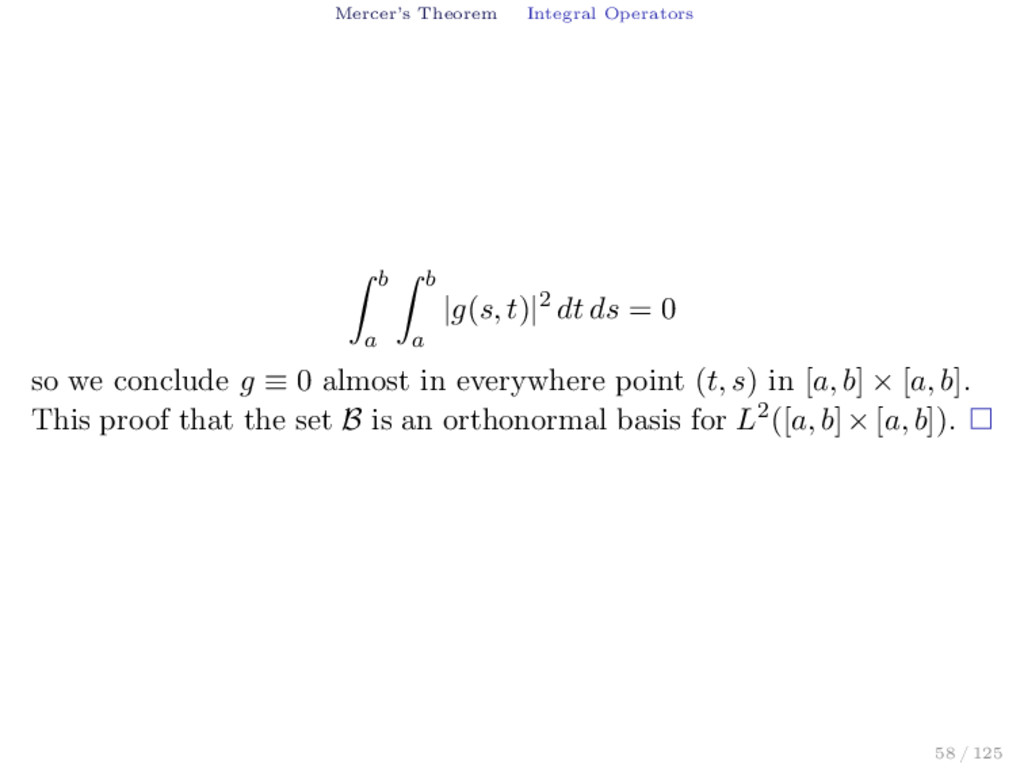
58. Mercer’s Theorem Integral Operators b a b a |g(s, t)|2 dt ds = 0 so we conclude g ≡ 0 almost in everywhere point (t, s) in [a, b] × [a, b]. This proof that the set B is an orthonormal basis for L2([a, b]×[a, b]). 58 / 125
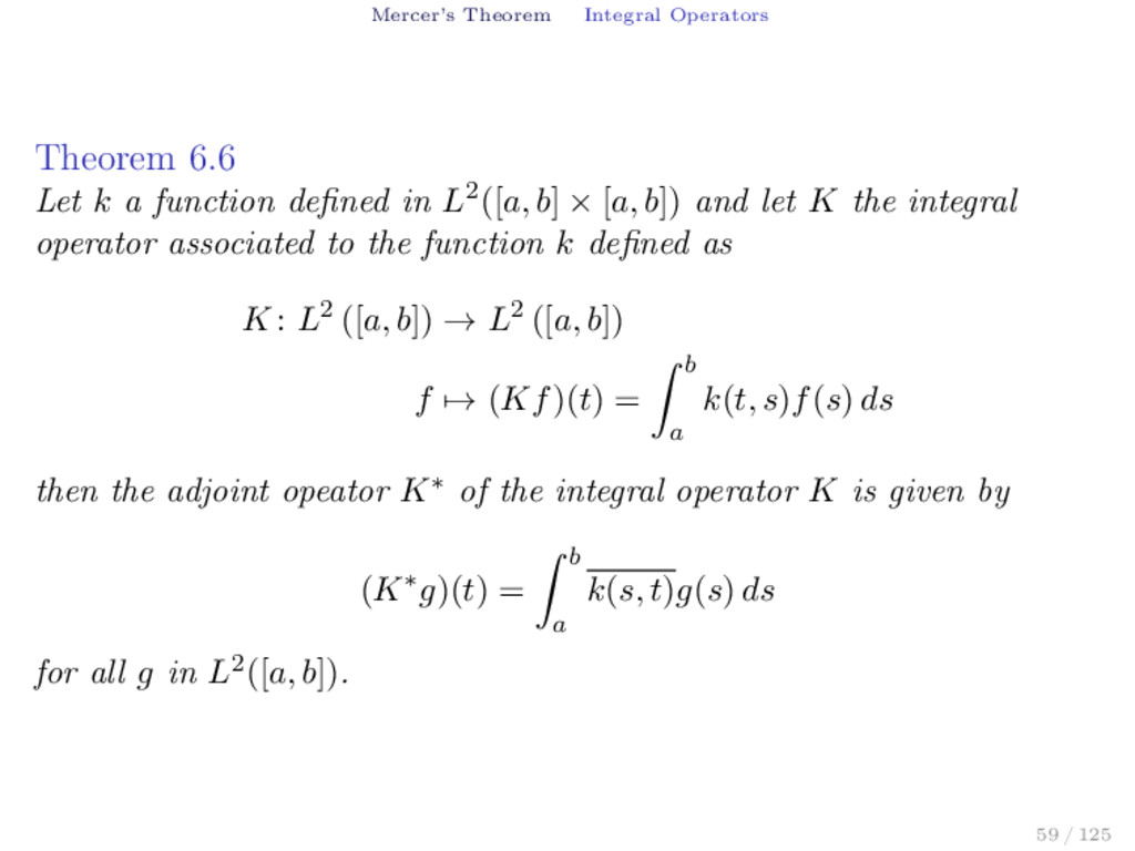
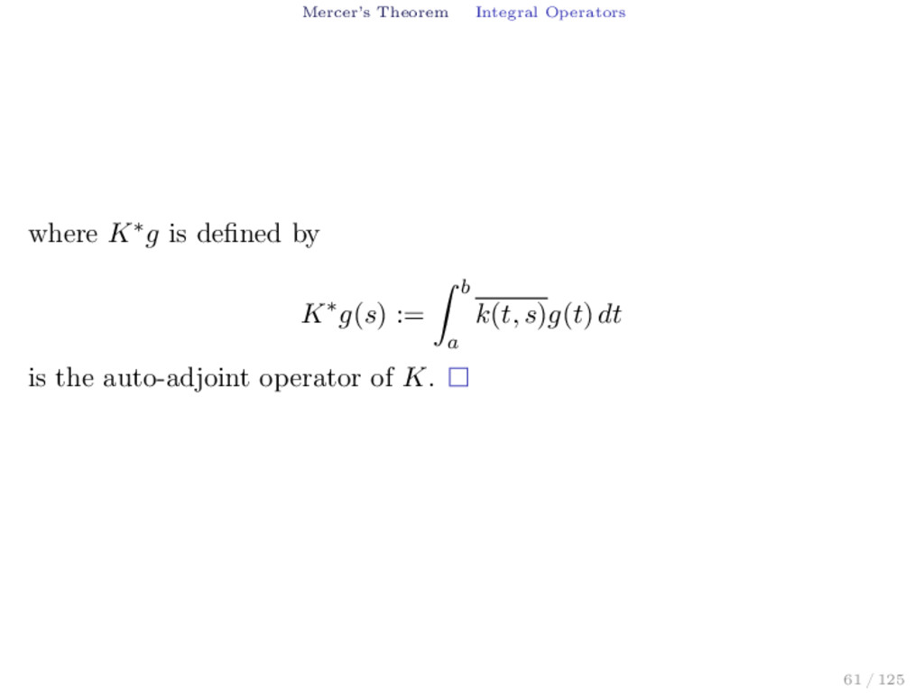
59. Mercer’s Theorem Integral Operators Theorem 6.6 Let k a function defined in L2([a, b] × [a, b]) and let K the integral operator associated to the function k defined as K : L2 ([a, b]) → L2 ([a, b]) f → (Kf)(t) = b a k(t, s)f(s) ds then the adjoint opeator K∗ of the integral operator K is given by (K∗g)(t) = b a k(s, t)g(s) ds for all g in L2([a, b]). 59 / 125
60. Mercer’s Theorem Integral Operators Proof. Kf, g L2([a,b]) = b a (Kf(t)) g(t) dt = b a b a k(t, s)f(s) ds g(t) dt = b a b a k(t, s)f(s)g(t) ds dt = b a b a k(t, s)f(s)g(t) dt ds (T. Fubini) = b a f(s) b a k(t, s)g(t) dt ds = b a f(s) b a k(t, s)g(t) dt ds = f, K∗g L2([a,b]) 60 / 125
61. Mercer’s Theorem Integral Operators where K∗g is defined by K∗g(s) := b a k(t, s)g(t) dt is the auto-adjoint operator of K. 61 / 125
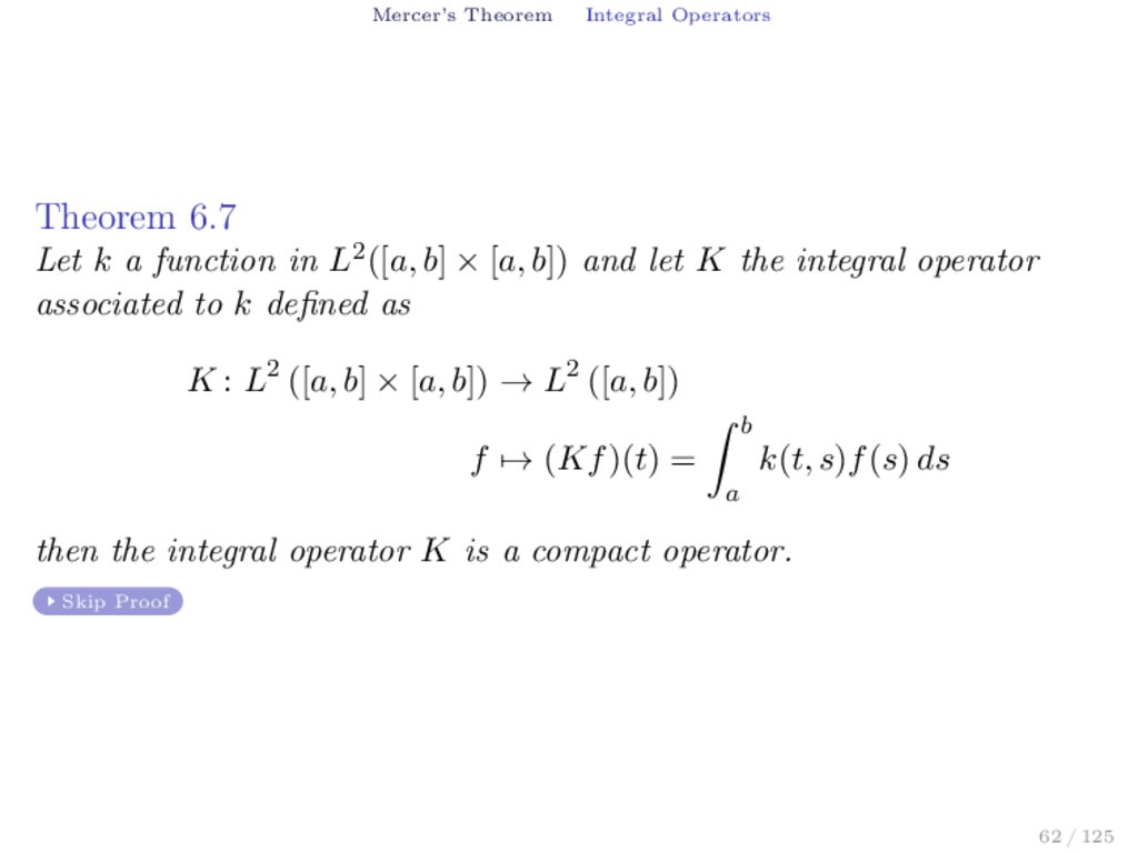
62. Mercer’s Theorem Integral Operators Theorem 6.7 Let k a function in L2([a, b] × [a, b]) and let K the integral operator associated to k defined as K : L2 ([a, b] × [a, b]) → L2 ([a, b]) f → (Kf)(t) = b a k(t, s)f(s) ds then the integral operator K is a compact operator. Skip Proof 62 / 125
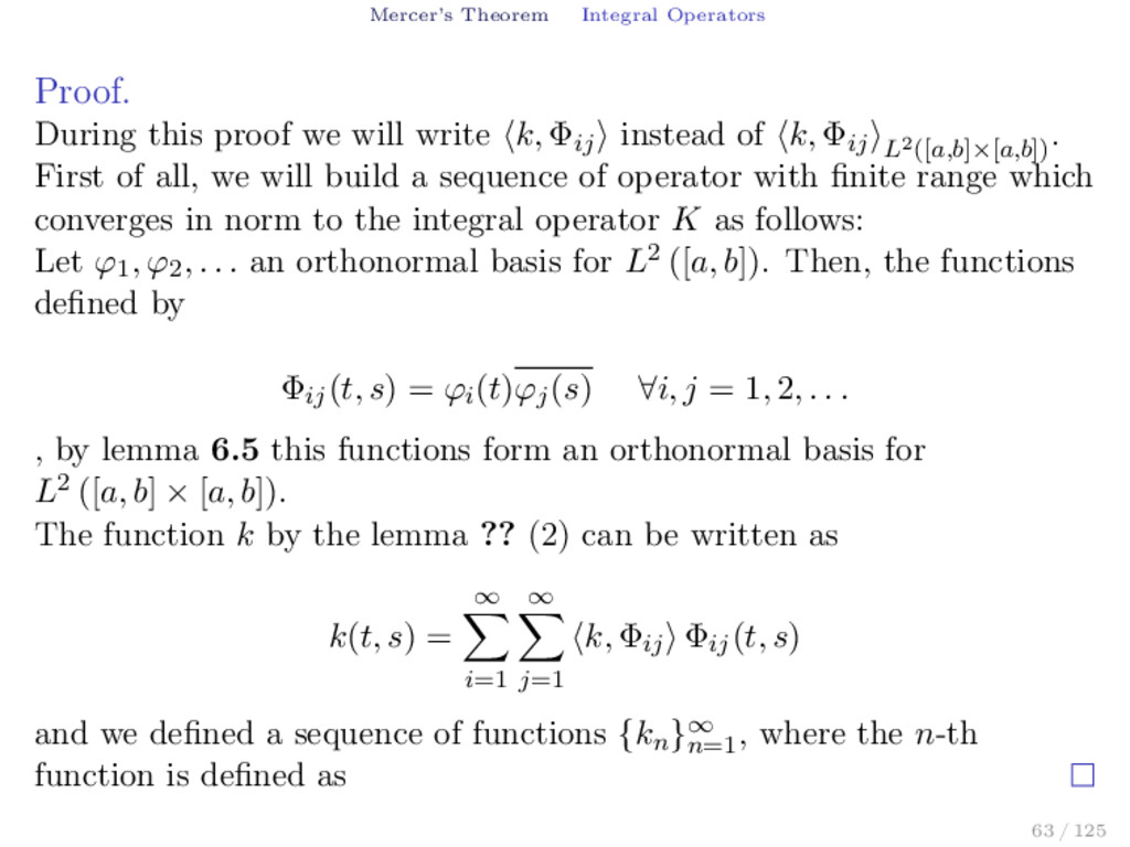
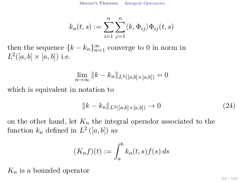
63. Mercer’s Theorem Integral Operators Proof. During this proof we will write k, Φij instead of k, Φij L2([a,b]×[a,b]) . First of all, we will build a sequence of operator with finite range which converges in norm to the integral operator K as follows: Let ϕ1 , ϕ2 , . . . an orthonormal basis for L2 ([a, b]). Then, the functions defined by Φij (t, s) = ϕi (t)ϕj (s) ∀i, j = 1, 2, . . . , by lemma 6.5 this functions form an orthonormal basis for L2 ([a, b] × [a, b]). The function k by the lemma ?? (2) can be written as k(t, s) = ∞ i=1 ∞ j=1 k, Φij Φij (t, s) and we defined a sequence of functions {kn }∞ n=1 , where the n-th function is defined as 63 / 125
64. Mercer’s Theorem Integral Operators kn (t, s) := n i=1 n j=1 k, Φij Φij (t, s) then the sequence {k − kn }∞ n=1 converge to 0 in norm in L2([a, b] × [a, b]) i.e. lim n→∞ k − kn L2([a,b]×[a,b]) = 0 which is equivalent in notation to k − kn L2([a,b]×[a,b]) → 0 (24) on the other hand, let Kn the integral operador associated to the function kn defined in L2 ([a, b]) as (Kn f)(t) := b a kn (t, s)f(s) ds Kn is a bounded operator 64 / 125
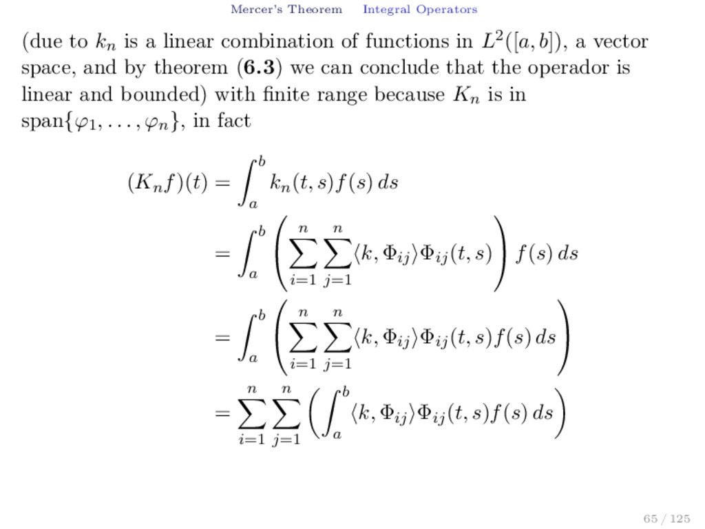
65. Mercer’s Theorem Integral Operators (due to kn is a linear combination of functions in L2([a, b]), a vector space, and by theorem (6.3) we can conclude that the operador is linear and bounded) with finite range because Kn is in span{ϕ1 , . . . , ϕn }, in fact (Kn f)(t) = b a kn (t, s)f(s) ds = b a   n i=1 n j=1 k, Φij Φij (t, s)   f(s) ds = b a   n i=1 n j=1 k, Φij Φij (t, s)f(s) ds   = n i=1 n j=1 b a k, Φij Φij (t, s)f(s) ds 65 / 125
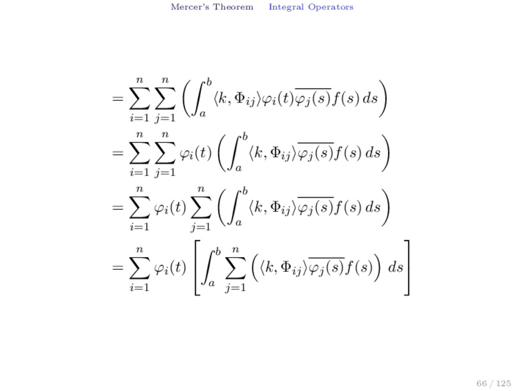
66. Mercer’s Theorem Integral Operators = n i=1 n j=1 b a k, Φij ϕi (t)ϕj (s)f(s) ds = n i=1 n j=1 ϕi (t) b a k, Φij ϕj (s)f(s) ds = n i=1 ϕi (t) n j=1 b a k, Φij ϕj (s)f(s) ds = n i=1 ϕi (t)   b a n j=1 k, Φij ϕj (s)f(s) ds   66 / 125
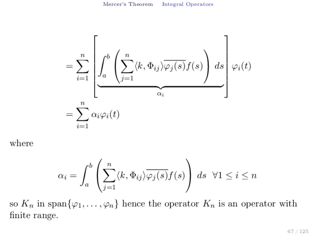
67. Mercer’s Theorem Integral Operators = n i=1        b a   n j=1 k, Φij ϕj (s)f(s)   ds αi        ϕi (t) = n i=1 αi ϕi (t) where αi = b a   n j=1 k, Φij ϕj (s)f(s)   ds ∀1 ≤ i ≤ n so Kn in span{ϕ1 , . . . , ϕn } hence the operator Kn is an operator with finite range. 67 / 125
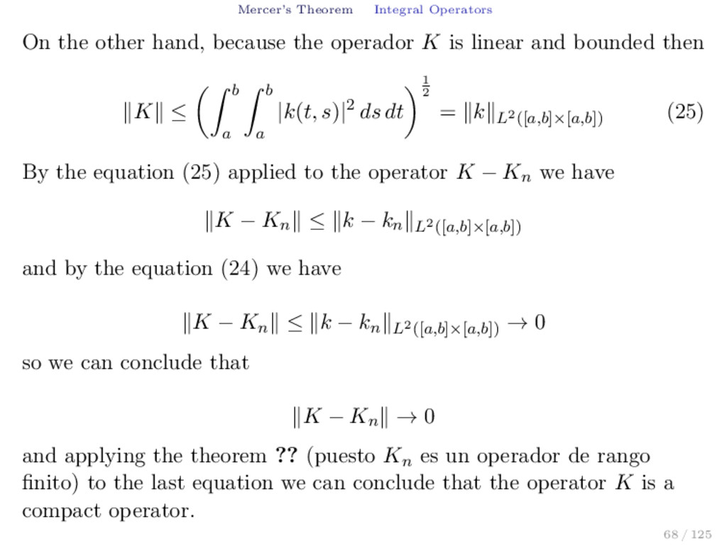
68. Mercer’s Theorem Integral Operators On the other hand, because the operador K is linear and bounded then K ≤ b a b a |k(t, s)|2 ds dt 1 2 = k L2([a,b]×[a,b]) (25) By the equation (25) applied to the operator K − Kn we have K − Kn ≤ k − kn L2([a,b]×[a,b]) and by the equation (24) we have K − Kn ≤ k − kn L2([a,b]×[a,b]) → 0 so we can conclude that K − Kn → 0 and applying the theorem ?? (puesto Kn es un operador de rango finito) to the last equation we can conclude that the operator K is a compact operator. 68 / 125
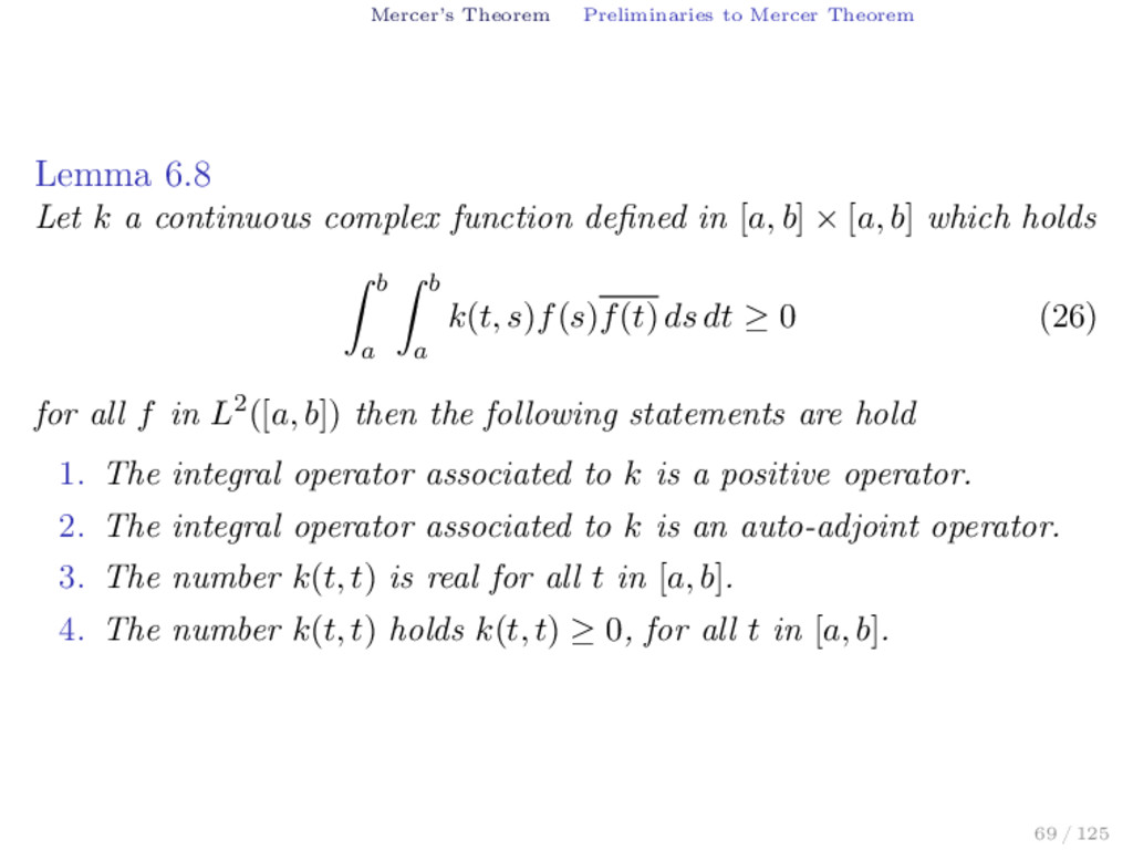
69. Mercer’s Theorem Preliminaries to Mercer Theorem Lemma 6.8 Let k a continuous complex function defined in [a, b] × [a, b] which holds b a b a k(t, s)f(s)f(t) ds dt ≥ 0 (26) for all f in L2([a, b]) then the following statements are hold 1. The integral operator associated to k is a positive operator. 2. The integral operator associated to k is an auto-adjoint operator. 3. The number k(t, t) is real for all t in [a, b]. 4. The number k(t, t) holds k(t, t) ≥ 0, for all t in [a, b]. 69 / 125
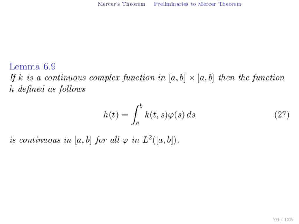
70. Mercer’s Theorem Preliminaries to Mercer Theorem Lemma 6.9 If k is a continuous complex function in [a, b] × [a, b] then the function h defined as follows h(t) = b a k(t, s)ϕ(s) ds (27) is continuous in [a, b] for all ϕ in L2([a, b]). 70 / 125
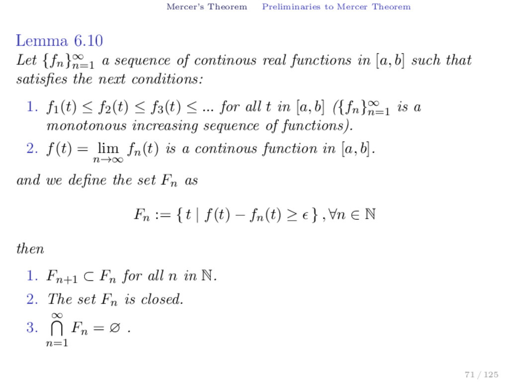
71. Mercer’s Theorem Preliminaries to Mercer Theorem Lemma 6.10 Let {fn }∞ n=1 a sequence of continous real functions in [a, b] such that satisfies the next conditions: 1. f1 (t) ≤ f2 (t) ≤ f3 (t) ≤ ... for all t in [a, b] ({fn }∞ n=1 is a monotonous increasing sequence of functions). 2. f(t) = lim n→∞ fn (t) is a continous function in [a, b]. and we define the set Fn as Fn := { t | f(t) − fn (t) ≥ } , ∀n ∈ N then 1. Fn+1 ⊂ Fn for all n in N. 2. The set Fn is closed. 3. ∞ n=1 Fn = ∅ . 71 / 125
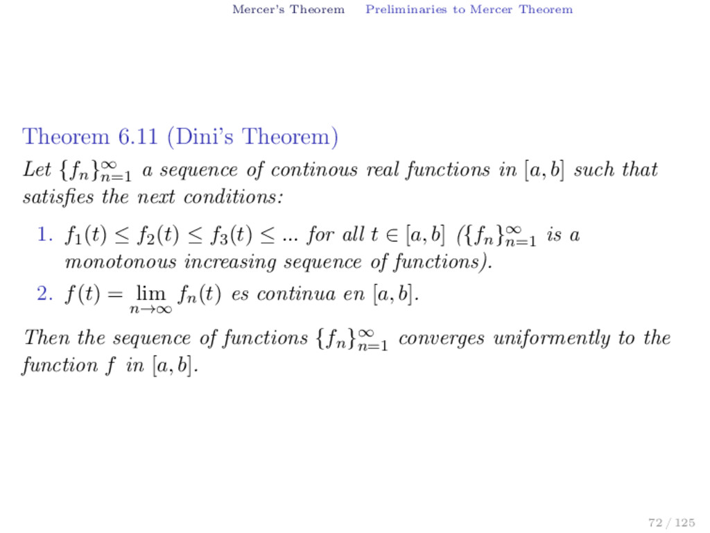
72. Mercer’s Theorem Preliminaries to Mercer Theorem Theorem 6.11 (Dini’s Theorem) Let {fn }∞ n=1 a sequence of continous real functions in [a, b] such that satisfies the next conditions: 1. f1 (t) ≤ f2 (t) ≤ f3 (t) ≤ ... for all t ∈ [a, b] ({fn }∞ n=1 is a monotonous increasing sequence of functions). 2. f(t) = lim n→∞ fn (t) es continua en [a, b]. Then the sequence of functions {fn }∞ n=1 converges uniformently to the function f in [a, b]. 72 / 125
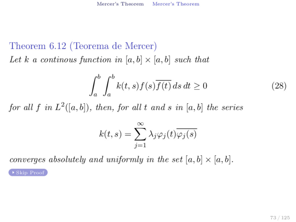
73. Mercer’s Theorem Mercer’s Theorem Theorem 6.12 (Teorema de Mercer) Let k a continous function in [a, b] × [a, b] such that b a b a k(t, s)f(s)f(t) ds dt ≥ 0 (28) for all f in L2([a, b]), then, for all t and s in [a, b] the series k(t, s) = ∞ j=1 λj ϕj (t)ϕj (s) converges absolutely and uniformly in the set [a, b] × [a, b]. Skip Proof 73 / 125
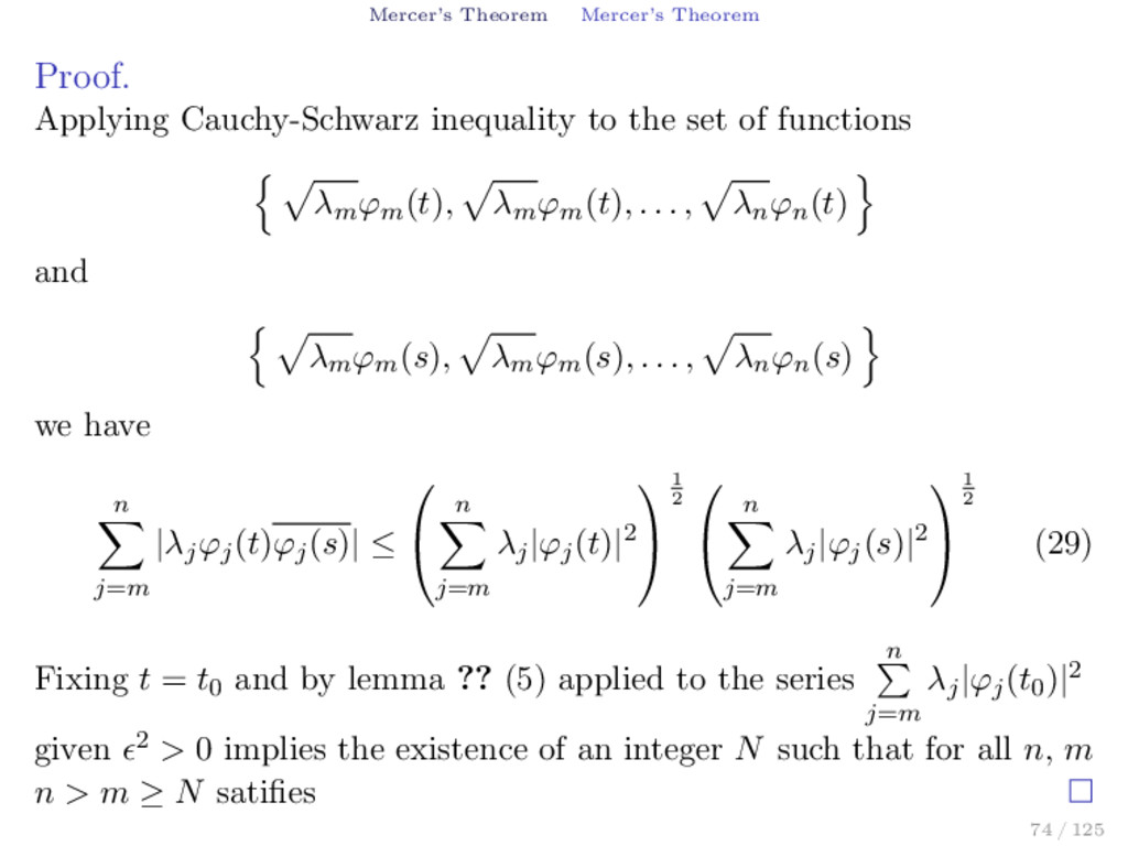
74. Mercer’s Theorem Mercer’s Theorem Proof. Applying Cauchy-Schwarz inequality to the set of functions λm ϕm (t), λm ϕm (t), . . . , λn ϕn (t) and λm ϕm (s), λm ϕm (s), . . . , λn ϕn (s) we have n j=m |λj ϕj (t)ϕj (s)| ≤   n j=m λj |ϕj (t)|2   1 2   n j=m λj |ϕj (s)|2   1 2 (29) Fixing t = t0 and by lemma ?? (5) applied to the series n j=m λj |ϕj (t0 )|2 given 2 > 0 implies the existence of an integer N such that for all n, m n > m ≥ N satifies 74 / 125
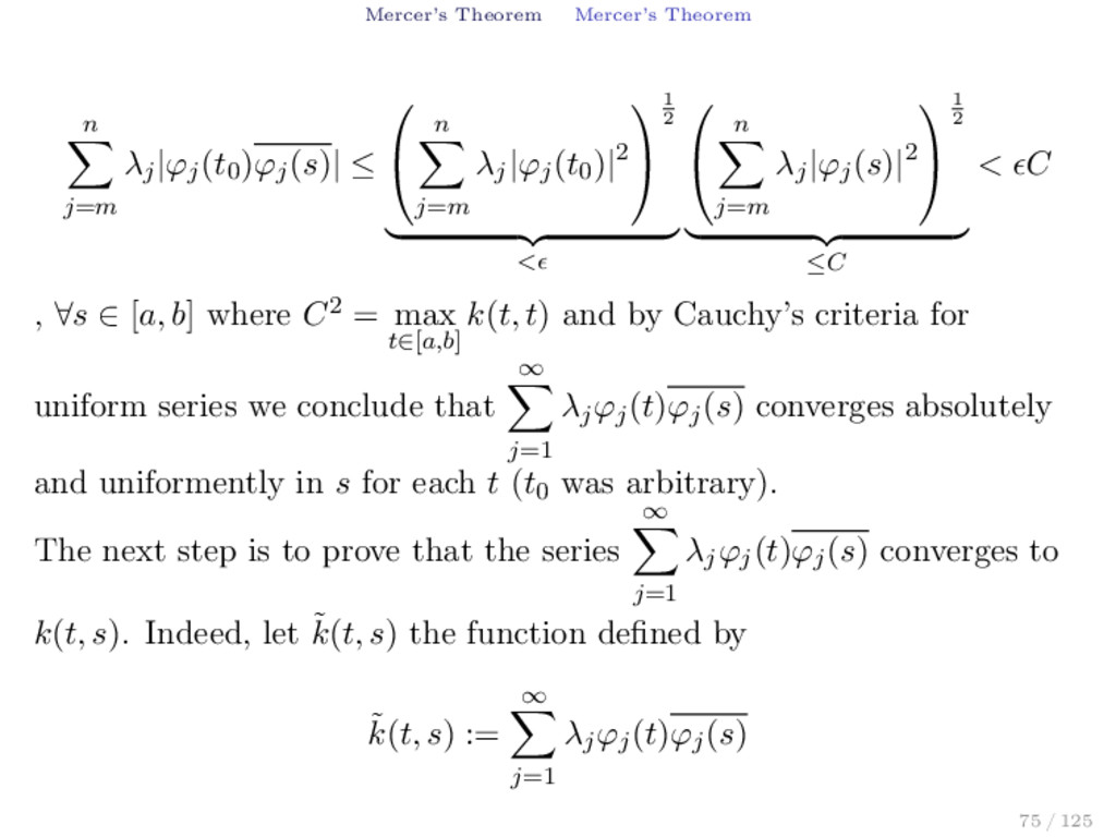
75. Mercer’s Theorem Mercer’s Theorem n j=m λj |ϕj (t0 )ϕj (s)| ≤   n j=m λj |ϕj (t0 )|2   1 2 <   n j=m λj |ϕj (s)|2   1 2 ≤C < C , ∀s ∈ [a, b] where C2 = max t∈[a,b] k(t, t) and by Cauchy’s criteria for uniform series we conclude that ∞ j=1 λj ϕj (t)ϕj (s) converges absolutely and uniformently in s for each t (t0 was arbitrary). The next step is to prove that the series ∞ j=1 λj ϕj (t)ϕj (s) converges to k(t, s). Indeed, let ˜ k(t, s) the function defined by ˜ k(t, s) := ∞ j=1 λj ϕj (t)ϕj (s) 75 / 125
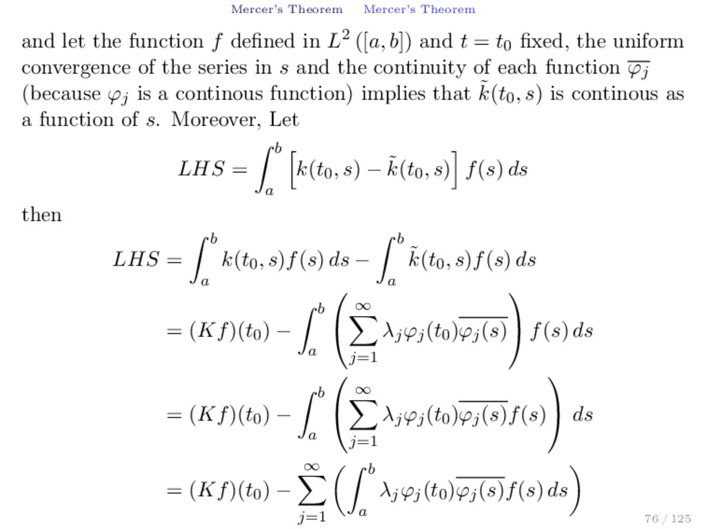
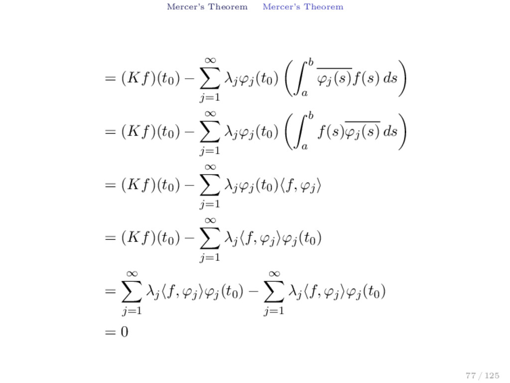
76. Mercer’s Theorem Mercer’s Theorem and let the function f defined in L2 ([a, b]) and t = t0 fixed, the uniform convergence of the series in s and the continuity of each function ϕj (because ϕj is a continous function) implies that ˜ k(t0 , s) is continous as a function of s. Moreover, Let LHS = b a k(t0 , s) − ˜ k(t0 , s) f(s) ds then LHS = b a k(t0 , s)f(s) ds − b a ˜ k(t0 , s)f(s) ds = (Kf)(t0 ) − b a   ∞ j=1 λj ϕj (t0 )ϕj (s)   f(s) ds = (Kf)(t0 ) − b a   ∞ j=1 λj ϕj (t0 )ϕj (s)f(s)   ds = (Kf)(t0 ) − ∞ j=1 b a λj ϕj (t0 )ϕj (s)f(s) ds 76 / 125
77. Mercer’s Theorem Mercer’s Theorem = (Kf)(t0 ) − ∞ j=1 λj ϕj (t0 ) b a ϕj (s)f(s) ds = (Kf)(t0 ) − ∞ j=1 λj ϕj (t0 ) b a f(s)ϕj (s) ds = (Kf)(t0 ) − ∞ j=1 λj ϕj (t0 ) f, ϕj = (Kf)(t0 ) − ∞ j=1 λj f, ϕj ϕj (t0 ) = ∞ j=1 λj f, ϕj ϕj (t0 ) − ∞ j=1 λj f, ϕj ϕj (t0 ) = 0 77 / 125
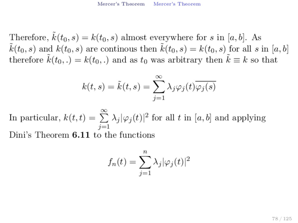
78. Mercer’s Theorem Mercer’s Theorem Therefore, ˜ k(t0 , s) = k(t0 , s) almost everywhere for s in [a, b]. As ˜ k(t0 , s) and k(t0 , s) are continous then ˜ k(t0 , s) = k(t0 , s) for all s in [a, b] therefore ˜ k(t0 , .) = k(t0 , .) and as t0 was arbitrary then ˜ k ≡ k so that k(t, s) = ˜ k(t, s) = ∞ j=1 λj ϕj (t)ϕj (s) In particular, k(t, t) = ∞ j=1 λj |ϕj (t)|2 for all t in [a, b] and applying Dini’s Theorem 6.11 to the functions fn (t) = n j=1 λj |ϕj (t)|2 78 / 125
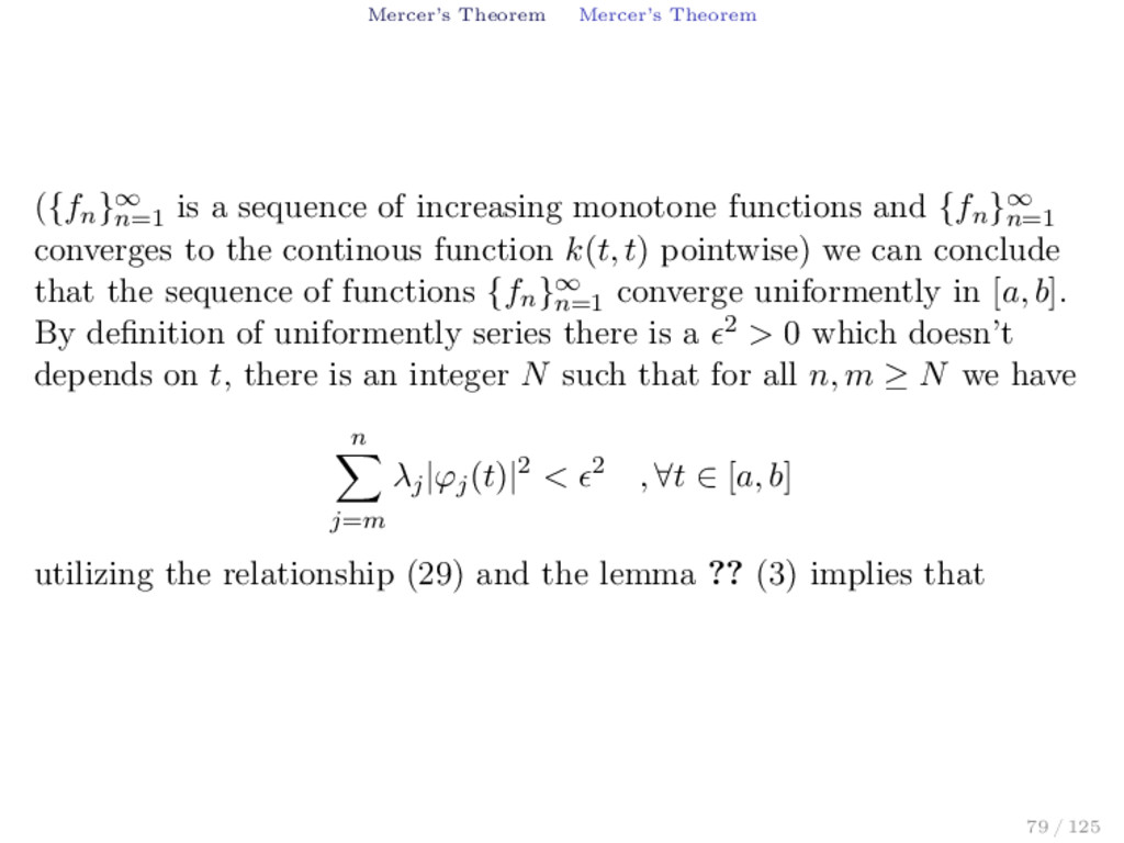
79. Mercer’s Theorem Mercer’s Theorem ({fn }∞ n=1 is a sequence of increasing monotone functions and {fn }∞ n=1 converges to the continous function k(t, t) pointwise) we can conclude that the sequence of functions {fn }∞ n=1 converge uniformently in [a, b]. By definition of uniformently series there is a 2 > 0 which doesn’t depends on t, there is an integer N such that for all n, m ≥ N we have n j=m λj |ϕj (t)|2 < 2 , ∀t ∈ [a, b] utilizing the relationship (29) and the lemma ?? (3) implies that 79 / 125
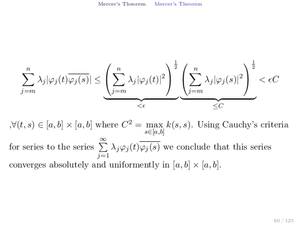
80. Mercer’s Theorem Mercer’s Theorem n j=m λj |ϕj (t)ϕj (s)| ≤   n j=m λj |ϕj (t)|2   1 2 <   n j=m λj |ϕj (s)|2   1 2 ≤C < C ,∀(t, s) ∈ [a, b] × [a, b] where C2 = max s∈[a,b] k(s, s). Using Cauchy’s criteria for series to the series ∞ j=1 λj ϕj (t)ϕj (s) we conclude that this series converges absolutely and uniformently in [a, b] × [a, b]. 80 / 125
81. References for Mercer’s Theorem References for Mercer’s Theorem Main Sources: [17] Israel Gohberg, Seymour Goldberg, and Marinus A. Kaashoek. Basic Classes of Linear Operators. Birkhäuser, 2003. [22] Harry Hochstadt. Integral Equations. Wiley, 1989. Minor Sources: [13] Nelson Dunford and Jacob T. Schwartz. Linear Opertors Part II: Spectral Theory Self Adjoint Operators in Hilbert Space. Interscience Publishers, 1963. [30] James Mercer. “Functions of positive and negative type and their connection with the theory of integral equations”. In: Philosophical Transactions of the Royal Society (1909), pp. 415–446. [55] Stephen M. Zemyan. The Classical Theory of Integral Equations: A Concise Treatment. Birkhauser, 2010. 81 / 125
82. Moore-Aronszajn Theorem
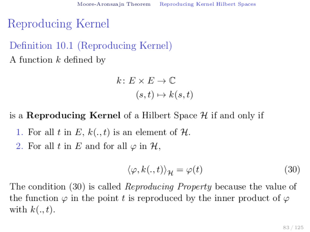
83. Moore-Aronszajn Theorem Reproducing Kernel Hilbert Spaces Reproducing Kernel Definition 10.1 (Reproducing Kernel) A function k defined by k: E × E → C (s, t) → k(s, t) is a Reproducing Kernel of a Hilbert Space H if and only if 1. For all t in E, k(., t) is an element of H. 2. For all t in E and for all ϕ in H, ϕ, k(., t) H = ϕ(t) (30) The condition (30) is called Reproducing Property because the value of the function ϕ in the point t is reproduced by the inner product of ϕ with k(., t). 83 / 125
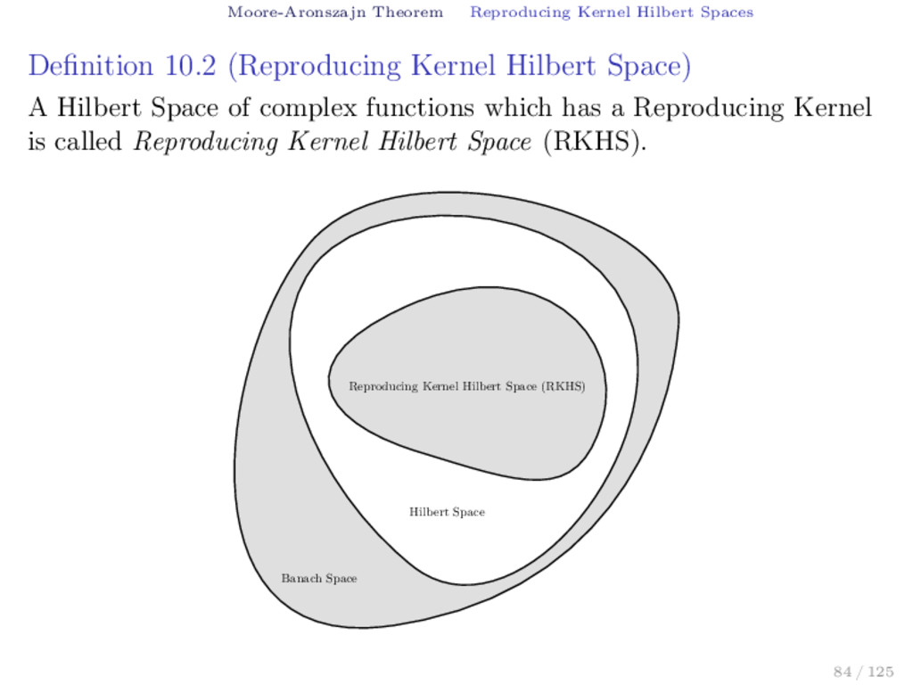
84. Moore-Aronszajn Theorem Reproducing Kernel Hilbert Spaces Definition 10.2 (Reproducing Kernel Hilbert Space) A Hilbert Space of complex functions which has a Reproducing Kernel is called Reproducing Kernel Hilbert Space (RKHS). Hilbert Space Banach Space Reproducing Kernel Hilbert Space (RKHS) 84 / 125
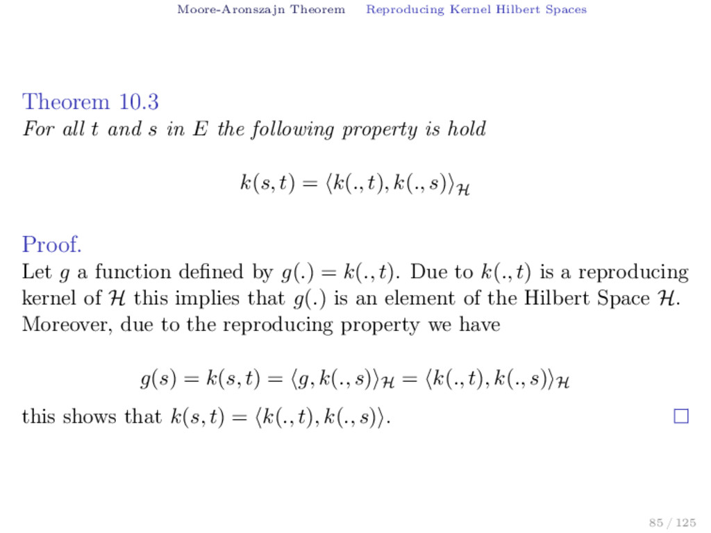
85. Moore-Aronszajn Theorem Reproducing Kernel Hilbert Spaces Theorem 10.3 For all t and s in E the following property is hold k(s, t) = k(., t), k(., s) H Proof. Let g a function defined by g(.) = k(., t). Due to k(., t) is a reproducing kernel of H this implies that g(.) is an element of the Hilbert Space H. Moreover, due to the reproducing property we have g(s) = k(s, t) = g, k(., s) H = k(., t), k(., s) H this shows that k(s, t) = k(., t), k(., s) . 85 / 125
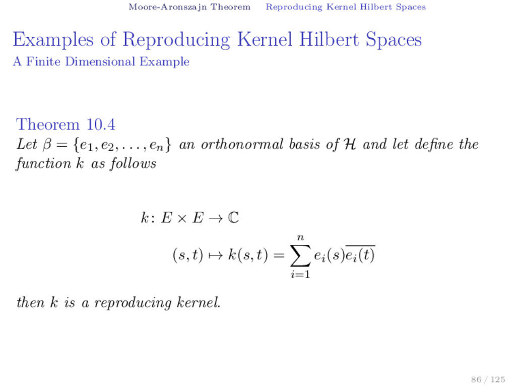
86. Moore-Aronszajn Theorem Reproducing Kernel Hilbert Spaces Examples of Reproducing Kernel Hilbert Spaces A Finite Dimensional Example Theorem 10.4 Let β = {e1 , e2 , . . . , en } an orthonormal basis of H and let define the function k as follows k: E × E → C (s, t) → k(s, t) = n i=1 ei (s)ei (t) then k is a reproducing kernel. 86 / 125
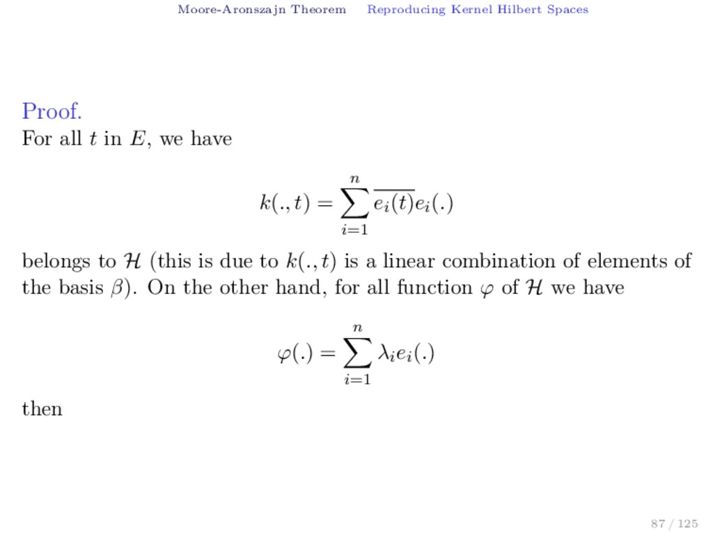
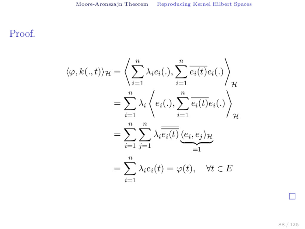
87. Moore-Aronszajn Theorem Reproducing Kernel Hilbert Spaces Proof. For all t in E, we have k(., t) = n i=1 ei (t)ei (.) belongs to H (this is due to k(., t) is a linear combination of elements of the basis β). On the other hand, for all function ϕ of H we have ϕ(.) = n i=1 λi ei (.) then 87 / 125
88. Moore-Aronszajn Theorem Reproducing Kernel Hilbert Spaces Proof. ϕ, k(., t) H = n i=1 λi ei (.), n i=1 ei (t)ei (.) H = n i=1 λi ei (.), n i=1 ei (t)ei (.) H = n i=1 n j=1 λi ei (t) ei , ej H =1 = n i=1 λi ei (t) = ϕ(t), ∀t ∈ E 88 / 125
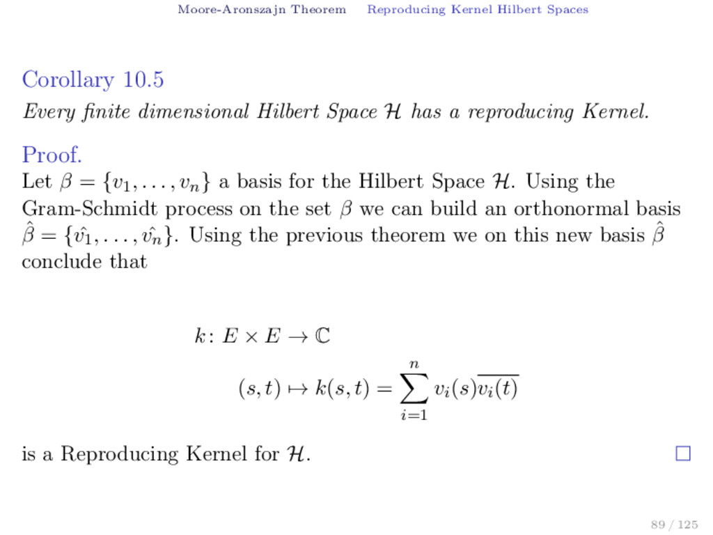
89. Moore-Aronszajn Theorem Reproducing Kernel Hilbert Spaces Corollary 10.5 Every finite dimensional Hilbert Space H has a reproducing Kernel. Proof. Let β = {v1 , . . . , vn } a basis for the Hilbert Space H. Using the Gram-Schmidt process on the set β we can build an orthonormal basis ˆ β = { ˆ v1 , . . . , ˆ vn }. Using the previous theorem we on this new basis ˆ β conclude that k: E × E → C (s, t) → k(s, t) = n i=1 vi (s)vi (t) is a Reproducing Kernel for H. 89 / 125
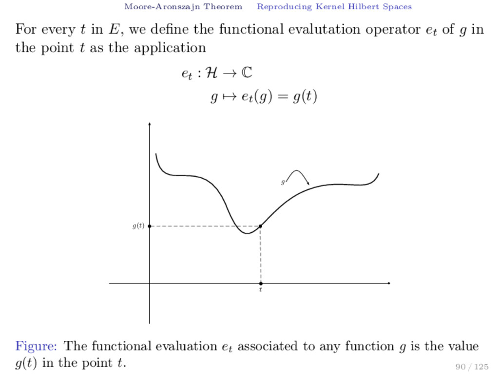
90. Moore-Aronszajn Theorem Reproducing Kernel Hilbert Spaces For every t in E, we define the functional evalutation operator et of g in the point t as the application et : H → C g → et (g) = g(t) g(t) t g Figure: The functional evaluation et associated to any function g is the value g(t) in the point t. 90 / 125
91. Moore-Aronszajn Theorem Reproducing Kernel Hilbert Spaces Theorem 10.6 A Hilbert spaces of complex function in E has a reproducing kernel if and only if all the functional evaluations et, t in E, are continous in H. 91 / 125
92. Moore-Aronszajn Theorem Reproducing Kernel Hilbert Spaces Corollary 10.7 Let H an RKHS then all sequence which converges in norm converge pointwise to the same limit. 92 / 125
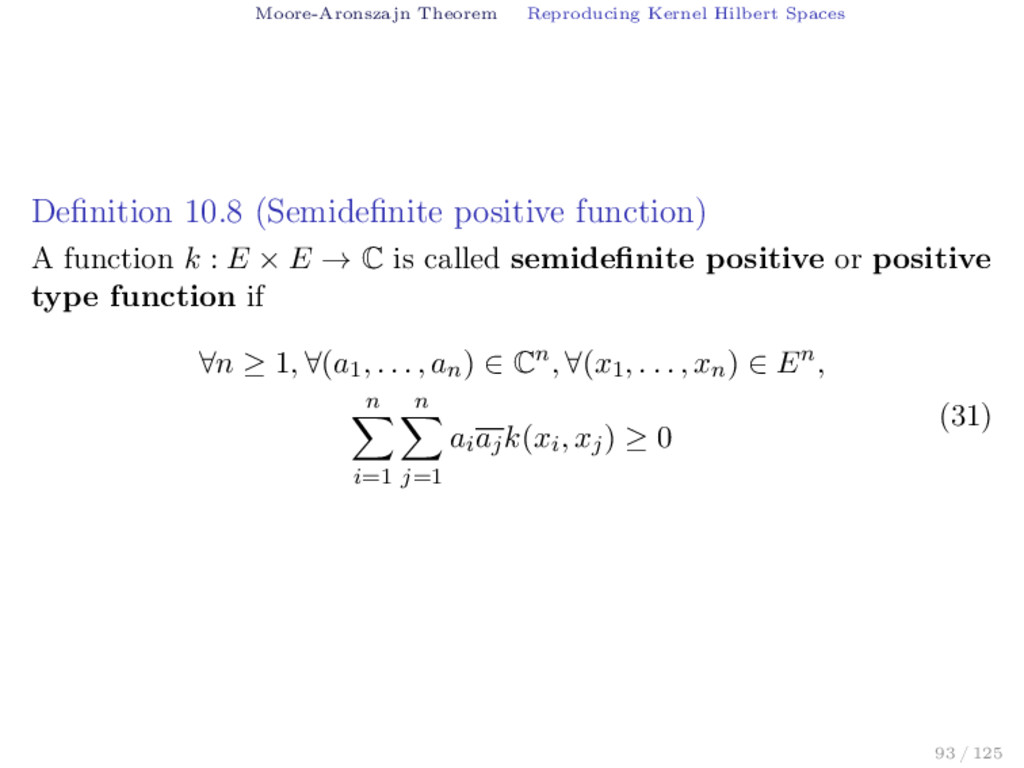
93. Moore-Aronszajn Theorem Reproducing Kernel Hilbert Spaces Definition 10.8 (Semidefinite positive function) A function k : E × E → C is called semidefinite positive or positive type function if ∀n ≥ 1, ∀(a1 , . . . , an ) ∈ Cn, ∀(x1 , . . . , xn ) ∈ En, n i=1 n j=1 ai aj k(xi , xj ) ≥ 0 (31) 93 / 125
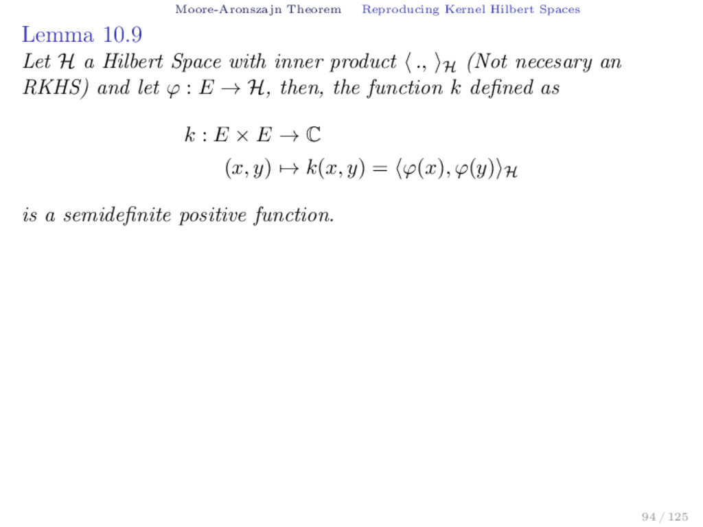
94. Moore-Aronszajn Theorem Reproducing Kernel Hilbert Spaces Lemma 10.9 Let H a Hilbert Space with inner product ., H (Not necesary an RKHS) and let ϕ : E → H, then, the function k defined as k : E × E → C (x, y) → k(x, y) = ϕ(x), ϕ(y) H is a semidefinite positive function. 94 / 125
95. Moore-Aronszajn Theorem Reproducing Kernel Hilbert Spaces Lemma 10.10 Every reproducing kernel is semidefinite positive. 95 / 125
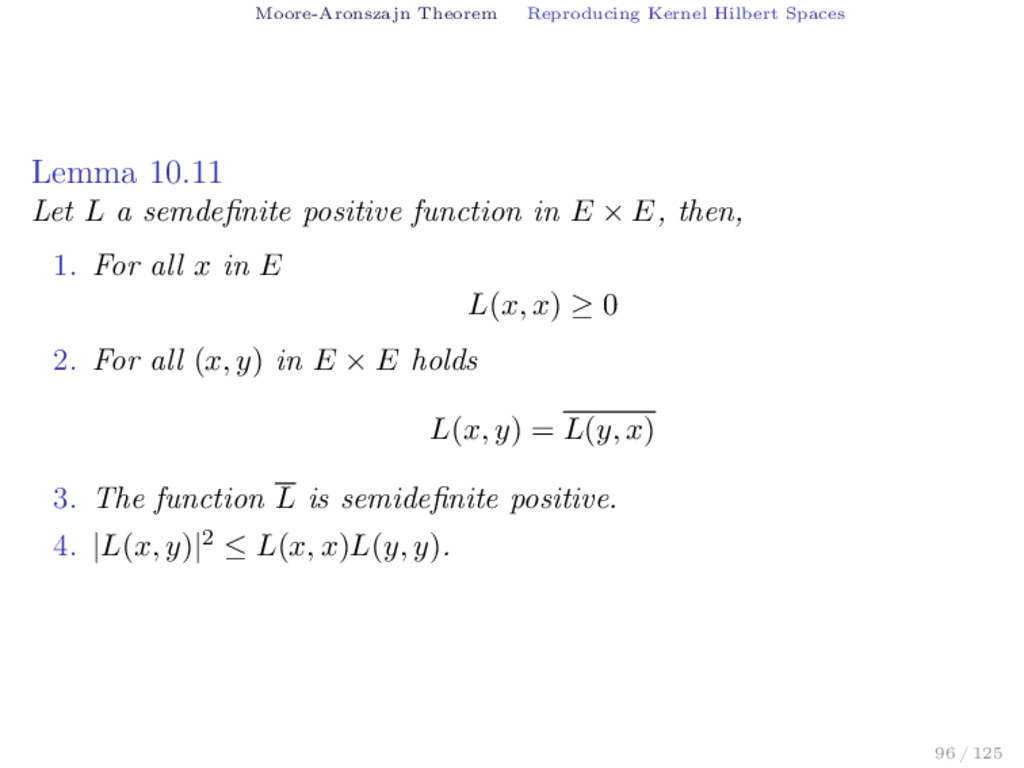
96. Moore-Aronszajn Theorem Reproducing Kernel Hilbert Spaces Lemma 10.11 Let L a semdefinite positive function in E × E, then, 1. For all x in E L(x, x) ≥ 0 2. For all (x, y) in E × E holds L(x, y) = L(y, x) 3. The function L is semidefinite positive. 4. |L(x, y)|2 ≤ L(x, x)L(y, y). 96 / 125
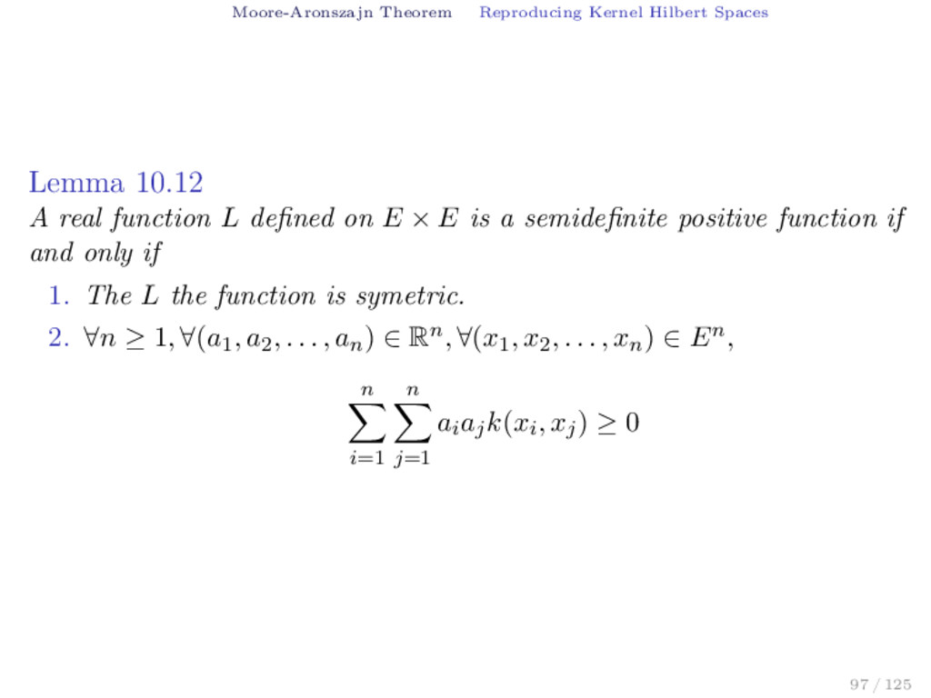
97. Moore-Aronszajn Theorem Reproducing Kernel Hilbert Spaces Lemma 10.12 A real function L defined on E × E is a semidefinite positive function if and only if 1. The L the function is symetric. 2. ∀n ≥ 1, ∀(a1 , a2 , . . . , an ) ∈ Rn, ∀(x1 , x2 , . . . , xn ) ∈ En, n i=1 n j=1 ai aj k(xi , xj ) ≥ 0 97 / 125
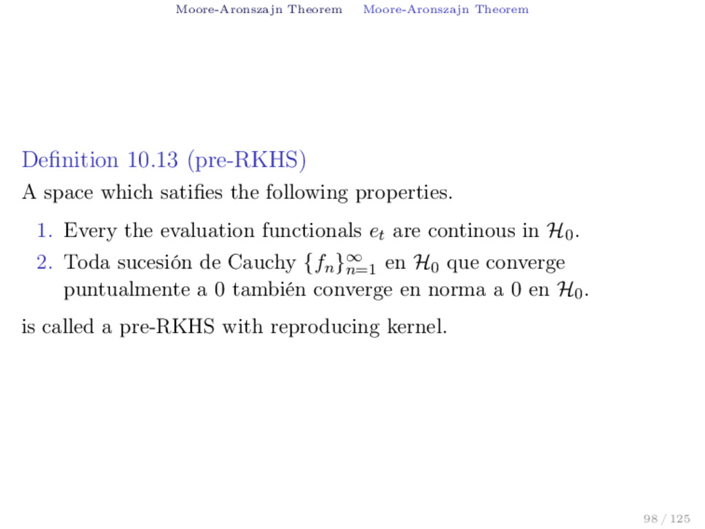
98. Moore-Aronszajn Theorem Moore-Aronszajn Theorem Definition 10.13 (pre-RKHS) A space which satifies the following properties. 1. Every the evaluation functionals et are continous in H0. 2. Toda sucesión de Cauchy {fn }∞ n=1 en H0 que converge puntualmente a 0 también converge en norma a 0 en H0. is called a pre-RKHS with reproducing kernel. 98 / 125
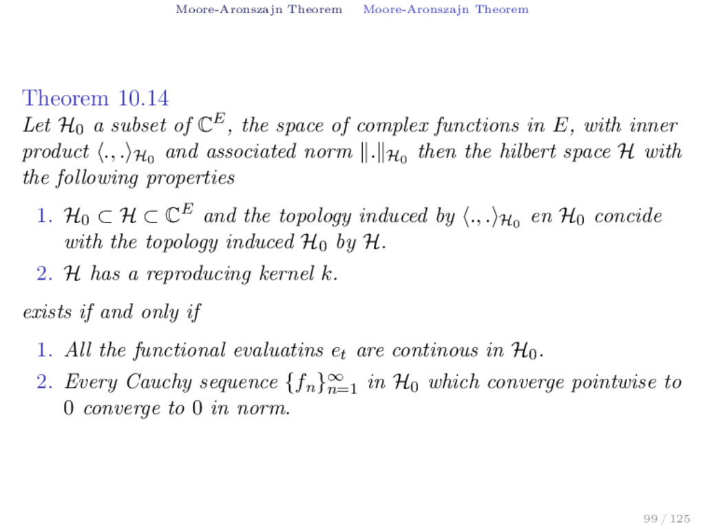
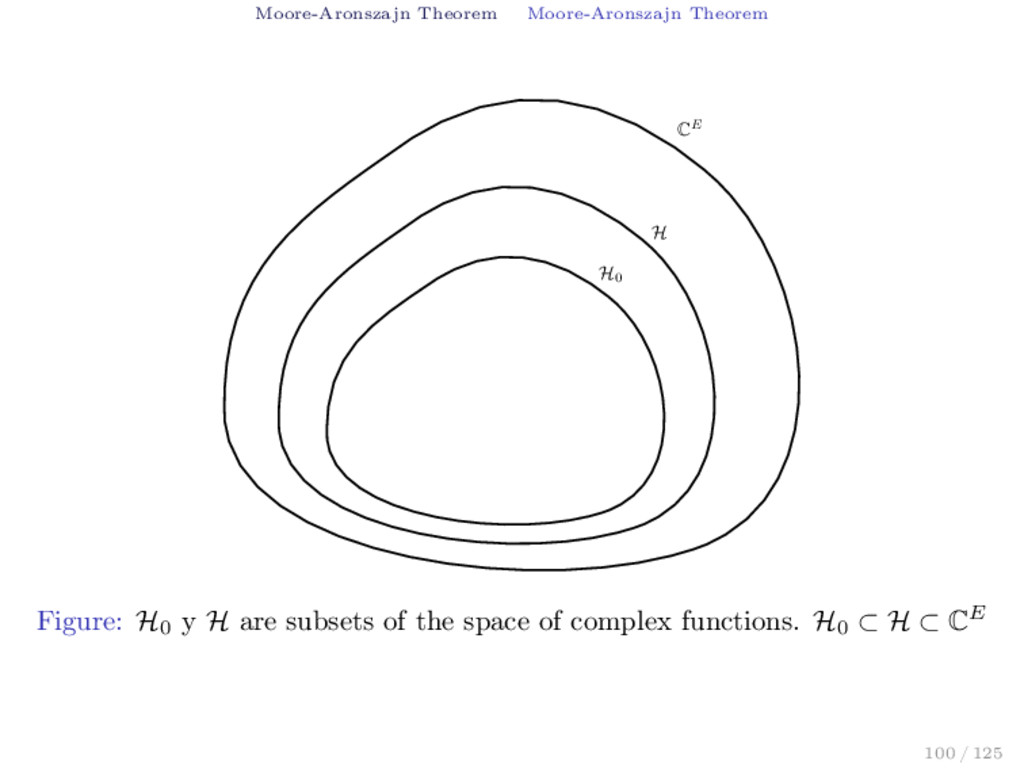
99. Moore-Aronszajn Theorem Moore-Aronszajn Theorem Theorem 10.14 Let H0 a subset of CE, the space of complex functions in E, with inner product ., . H0 and associated norm . H0 then the hilbert space H with the following properties 1. H0 ⊂ H ⊂ CE and the topology induced by ., . H0 en H0 concide with the topology induced H0 by H. 2. H has a reproducing kernel k. exists if and only if 1. All the functional evaluatins et are continous in H0. 2. Every Cauchy sequence {fn }∞ n=1 in H0 which converge pointwise to 0 converge to 0 in norm. 99 / 125
100. Moore-Aronszajn Theorem Moore-Aronszajn Theorem H H0 CE Figure: H0 y H are subsets of the space of complex functions. H0 ⊂ H ⊂ CE 100 / 125
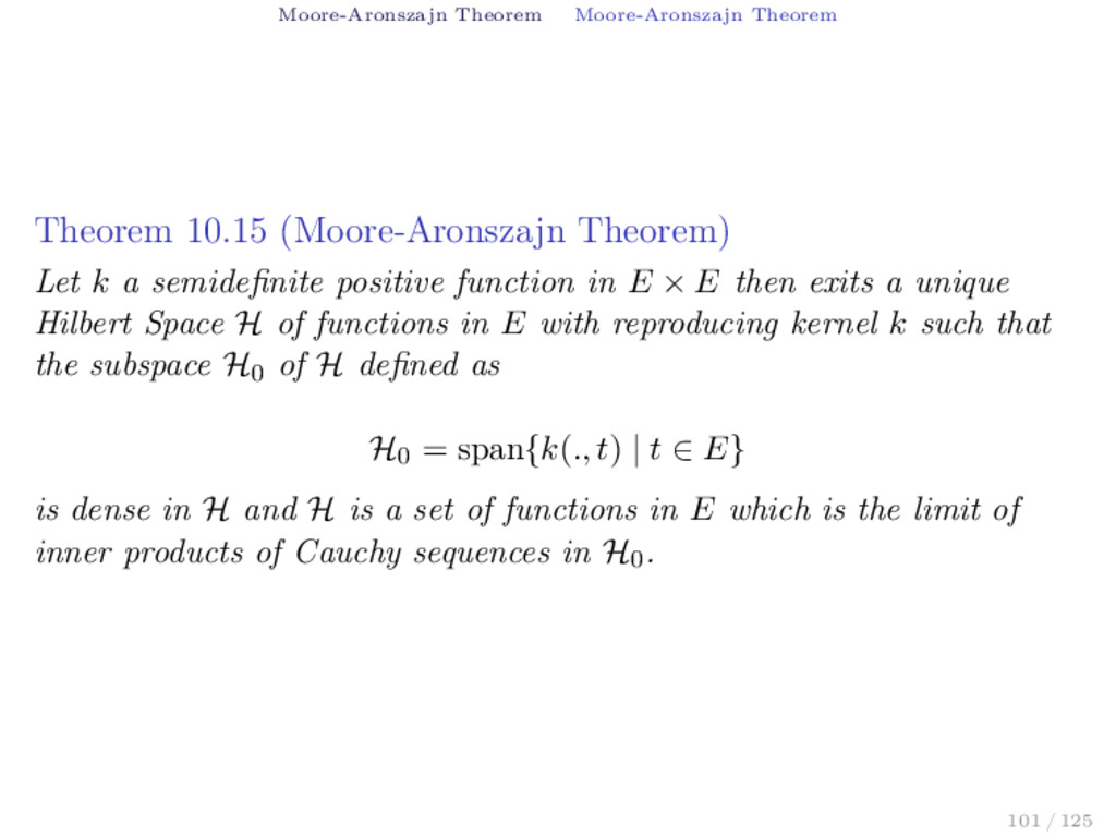
101. Moore-Aronszajn Theorem Moore-Aronszajn Theorem Theorem 10.15 (Moore-Aronszajn Theorem) Let k a semidefinite positive function in E × E then exits a unique Hilbert Space H of functions in E with reproducing kernel k such that the subspace H0 of H defined as H0 = span{k(., t) | t ∈ E} is dense in H and H is a set of functions in E which is the limit of inner products of Cauchy sequences in H0. 101 / 125
102. References for Moore-Aronszajn Theorem References for Moore-Aronszajn Theorem Main Sources: [4] Alain Berlinet and Christine Thomas. Reproducing kernel Hilbert spaces in Probability and Statistics. Kluwer Academic Publishers, 2004. [42] D. Sejdinovic and A. Gretton. Foundations of Reproducing Kernel Hilbert Space I. url: http://www.stats.ox.ac.uk/~sejdinov/RKHS_Slides1.pdf (visited on 03/11/2012). [43] D. Sejdinovic and A. Gretton. Foundations of Reproducing Kernel Hilbert Space II. url: http://www.gatsby.ucl.ac.uk/ ~gretton/coursefiles/RKHS_Slides2.pdf (visited on 03/11/2012). [44] D. Sejdinovic and A. Gretton. What is an RKHS? url: http://www.gatsby.ucl.ac.uk/~gretton/coursefiles/RKHS_ Notes1.pdf (visited on 03/11/2012). 102 / 125
103. The kernel Trick
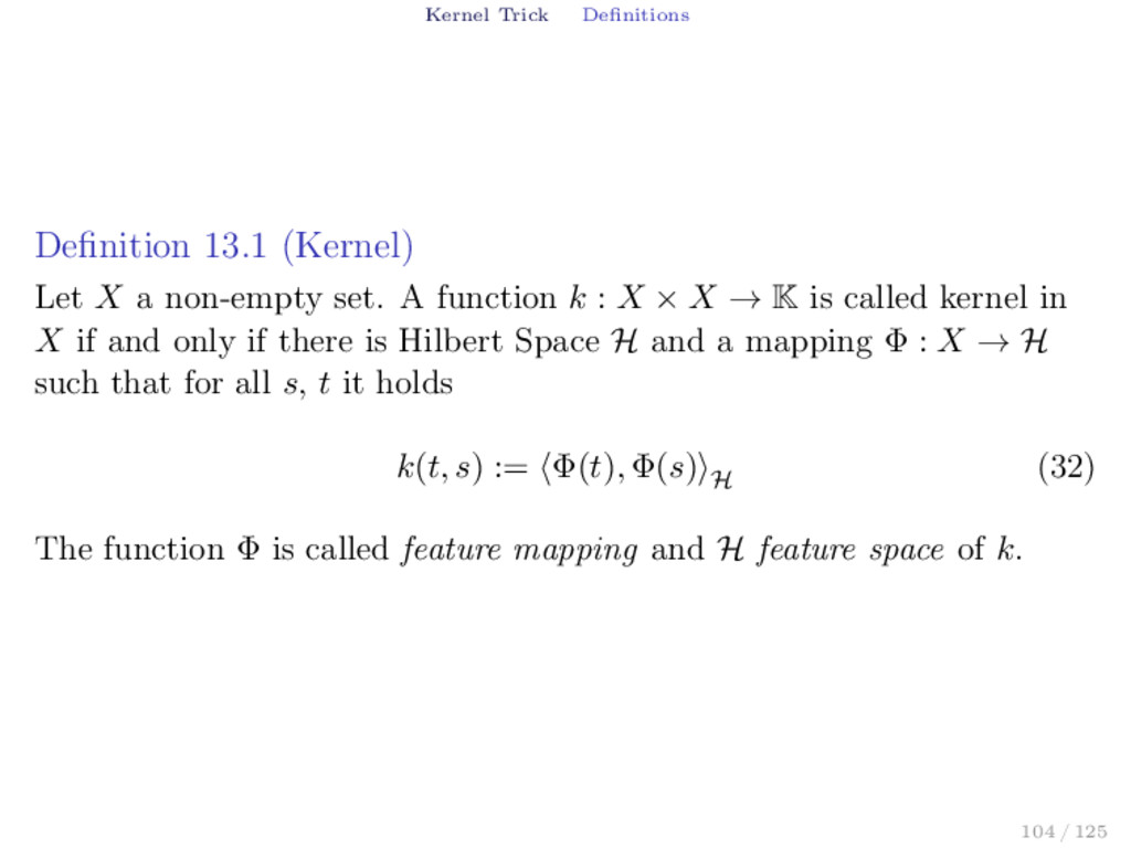
104. Kernel Trick Definitions Definition 13.1 (Kernel) Let X a non-empty set. A function k : X × X → K is called kernel in X if and only if there is Hilbert Space H and a mapping Φ : X → H such that for all s, t it holds k(t, s) := Φ(t), Φ(s) H (32) The function Φ is called feature mapping and H feature space of k. 104 / 125
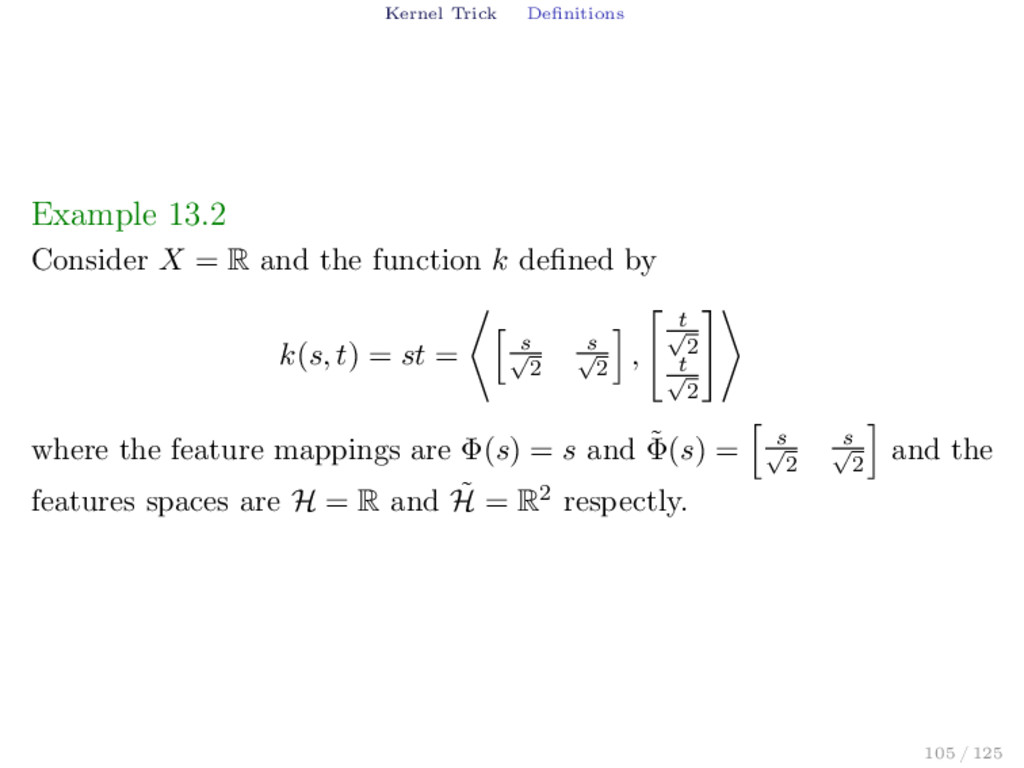
105. Kernel Trick Definitions Example 13.2 Consider X = R and the function k defined by k(s, t) = st = s √ 2 s √ 2 , t √ 2 t √ 2 where the feature mappings are Φ(s) = s and ˜ Φ(s) = s √ 2 s √ 2 and the features spaces are H = R and ˜ H = R2 respectly. 105 / 125
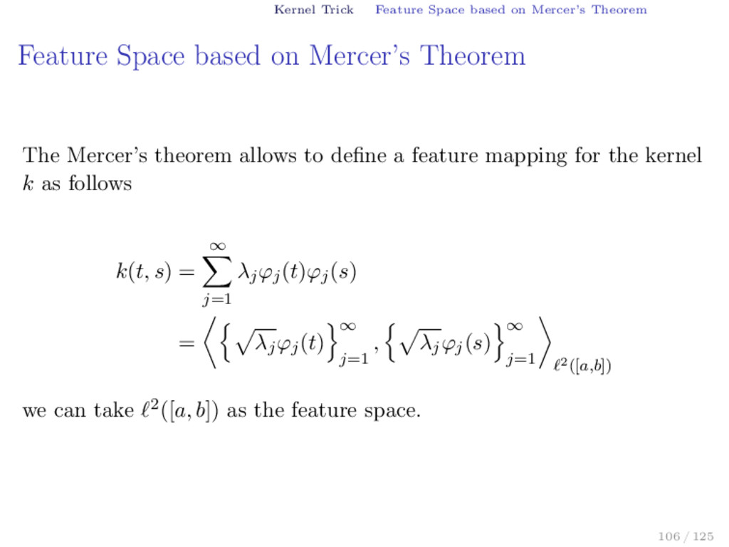
106. Kernel Trick Feature Space based on Mercer’s Theorem Feature Space based on Mercer’s Theorem The Mercer’s theorem allows to define a feature mapping for the kernel k as follows k(t, s) = ∞ j=1 λj ϕj (t)ϕj (s) = λj ϕj (t) ∞ j=1 , λj ϕj (s) ∞ j=1 2([a,b]) we can take 2([a, b]) as the feature space. 106 / 125
107. Kernel Trick Feature Space based on Mercer’s Theorem Theorem 13.3 The application Φ defined as Φ : [a, b] → 2([a, b]) t → λj ϕj (t) ∞ j=1 es well defined and satifies k(t, s) = Φ(t), Φ(s) 2([a,b]) (33) 107 / 125
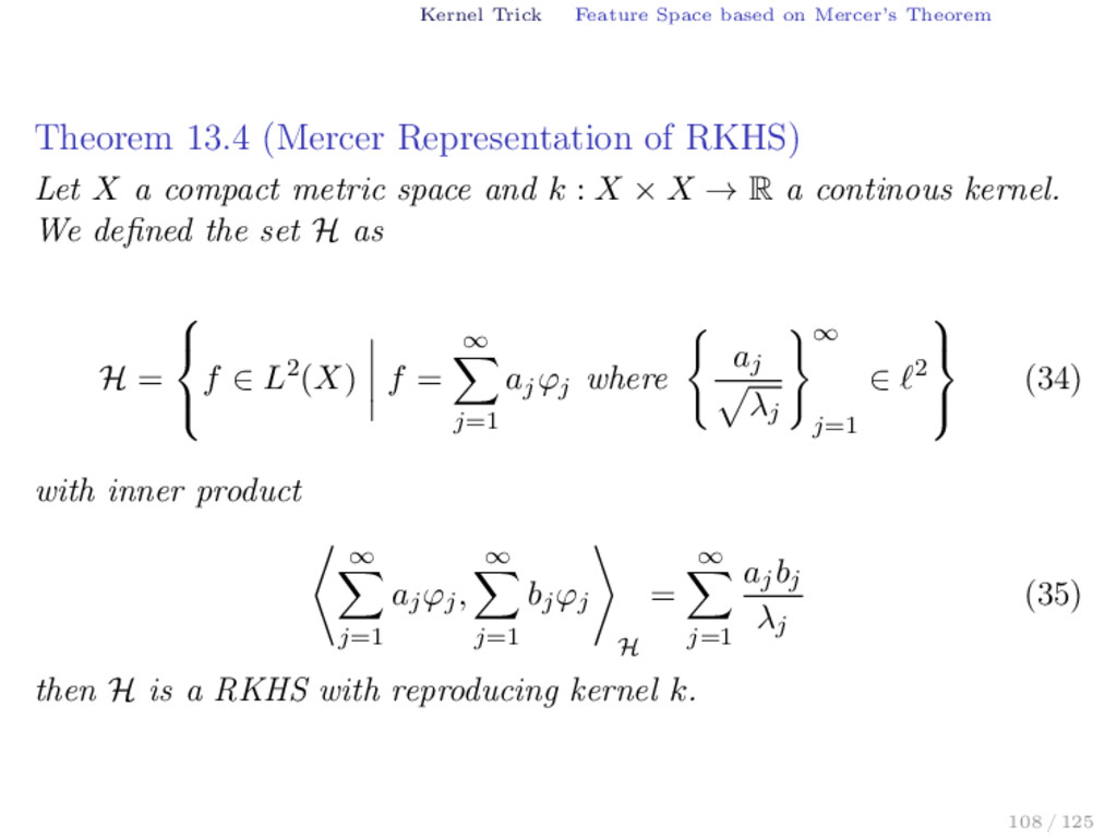
108. Kernel Trick Feature Space based on Mercer’s Theorem Theorem 13.4 (Mercer Representation of RKHS) Let X a compact metric space and k : X × X → R a continous kernel. We defined the set H as H =    f ∈ L2(X) f = ∞ j=1 aj ϕj where aj λj ∞ j=1 ∈ 2    (34) with inner product ∞ j=1 aj ϕj , ∞ j=1 bj ϕj H = ∞ j=1 aj bj λj (35) then H is a RKHS with reproducing kernel k. 108 / 125
109. History
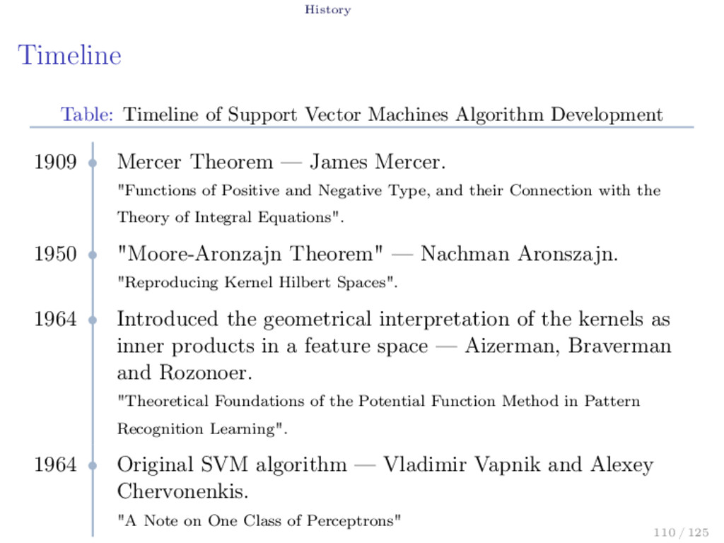
110. History Timeline Table: Timeline of Support Vector Machines Algorithm Development 1909 • Mercer Theorem — James Mercer. "Functions of Positive and Negative Type, and their Connection with the Theory of Integral Equations". 1950 • "Moore-Aronzajn Theorem" — Nachman Aronszajn. "Reproducing Kernel Hilbert Spaces". 1964 • Introduced the geometrical interpretation of the kernels as inner products in a feature space — Aizerman, Braverman and Rozonoer. "Theoretical Foundations of the Potential Function Method in Pattern Recognition Learning". 1964 • Original SVM algorithm — Vladimir Vapnik and Alexey Chervonenkis. "A Note on One Class of Perceptrons" 110 / 125
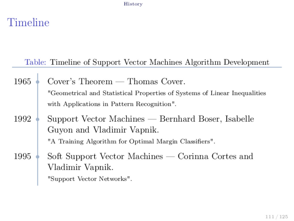
111. History Timeline Table: Timeline of Support Vector Machines Algorithm Development 1965 • Cover’s Theorem — Thomas Cover. "Geometrical and Statistical Properties of Systems of Linear Inequalities with Applications in Pattern Recognition". 1992 • Support Vector Machines — Bernhard Boser, Isabelle Guyon and Vladimir Vapnik. "A Training Algorithm for Optimal Margin Classifiers". 1995 • Soft Support Vector Machines — Corinna Cortes and Vladimir Vapnik. "Support Vector Networks". 111 / 125
112. References
113. References References I [1] Yaser S. Abu-Mostafa, Malik Magdon-Ismail, and Hsuan-Tien Lin. Learning From Data: A short course. AML Book, 2012. [2] Nachman Aronszajn. “Theory of Reproducing Kernels”. In: Transactions of the American Mathematical Society 68 (1950), pp. 337–404. [3] C. Berg, J. Reus, and P. Ressel. Harmonic Analysis on Semigroups: Theory of Positive Definite and Related Functions. Springer Science+Business Media, LLV, 1984. [4] Alain Berlinet and Christine Thomas. Reproducing kernel Hilbert spaces in Probability and Statistics. Kluwer Academic Publishers, 2004. [5] Donald L. Cohn. Measure Theory. Birkhäuser, 2013. 113 / 125
114. References References II [6] Corinna Cortes and Vladimir Vapnik. “Support Vector Networks”. In: Machine Learning (1995), pp. 273–297. [7] Thomas Cover. “Geometrical and Statistical properties of systems of linear inequalities with applications in pattern recognition”. In: IEEE Transactions on Electronic Computer (), pp. 326–334. [8] Nello Cristianini and John Shawe-Taylor. An Introduction to Support Vector Machines and Other Kernel-based Learning Methods. Cambridge University Press, 2000. [9] Felipe Cucker and Ding Xuan Zhou. Learning Theory. Cambridge University Press, 2007. [10] Steve Cucker Felipe; Smale. “On the Mathematical Foundations of Learning”. In: Bulletin of the American Mathematical Society (), pp. 1–49. 114 / 125
115. References References III [11] Naiyang Deng, Yingjie Tian, and Chunhua Zhang. Support Vector Machines: Optimization Based Theory, Algorithms, and Extensions. CRC Press, 2013. [12] Ke-Lin Du and M. N. S. Swamy. Neural Networks and Statistical Learning. Springer Science & Business Media, 2013. [13] Nelson Dunford and Jacob T. Schwartz. Linear Opertors Part II: Spectral Theory Self Adjoint Operators in Hilbert Space. Interscience Publishers, 1963. [14] Lawrence C. Evans. Partial Differential Equations. American Mathematical Society, 1998. [15] Gregory Fasshauer. Positive Definite Kernels: Past, Present and Future. url: http://www.math.iit.edu/~fass/PDKernels.pdf. 115 / 125
116. References References IV [16] Gregory E. Fasshauer. Positive Definite Kernels: Past, Present and Future. url: http://www.math.iit.edu/~fass/PDKernels.pdf. [17] Israel Gohberg, Seymour Goldberg, and Marinus A. Kaashoek. Basic Classes of Linear Operators. Birkhäuser, 2003. [18] Lutz Hamel. Knowledge Discovery with Support Vector Machines. Wiley-Interscience, 2009. [19] Simon Haykin. Neural Networks and Learning Machines. Third Edition. Pearson Prentice Hall, 2009. [20] Operadores integrais positivos e espaços de Hilbert de reprodução. “José Claudinei Ferreira”. PhD thesis. USP - São Carlos, 2010. 116 / 125
117. References References V [21] David Hilbert. “Grundzüge einer allgeminen Theorie der linaren Integralrechnungen.” In: Nachrichten, Math.-Phys. Kl (1904), pp. 49–91. url: http: //www.digizeitschriften.de/dms/img/?PPN=GDZPPN002499967. [22] Harry Hochstadt. Integral Equations. Wiley, 1989. [23] Alexey Izmailov and Mikhail Solodov. Otimização Vol.1 Condições de Otimalidade, Elementos de Analise Convexa e de Dualidade. Third Edition. IMPA, 2014. [24] Thorsten Joachims. Learning to Classify Text Using Support Vector Machines: Methods, Theory and Algorithms. Kluwer Academic Publishers, 2002. [25] J. Zico Kolter. MLSS 2014 – Introduction to Machine Learning. url: http://www.mlss2014.com/files/kolter_slides1.pdf. 117 / 125
118. References References VI [26] Hermann König. Eigenvalue Distribution of Compact Operators. Birkhäuser, 1986. [27] Elon Lages. Analisis Real, Volumen 1. Textos del IMCA, 1997. [28] Peter D. Lax. Functional Analysis. Wiley, 2002. [29] Le, Sarlos, and Smola. “Fastfood - Approximating Kernel Expansions in Loglinear Time”. In: ICML 2013 (). [30] James Mercer. “Functions of positive and negative type and their connection with the theory of integral equations”. In: Philosophical Transactions of the Royal Society (1909), pp. 415–446. [31] Mehryar Mohri, Afshin Rostamizadeh, and Ameet Talwalkar. Foundations of Machine Learning. The MIT Press, 2012. 118 / 125
119. References References VII [32] F. Pedregosa et al. “Scikit-learn: Machine Learning in Python”. In: Journal of Machine Learning Research 12 (2011), pp. 2825–2830. [33] Anthony L. Peressini, Francis E. Sullivan, and J.J. Jr. Uhl. The Mathematics of Nonlinear Programming. Springer, 1993. [34] David Porter and David S. G. Stirling. Integral Equations: A practical treatment, from spectral theory to applications. Cambridge University Press, 1990. [35] Carl Edward Rasmussen and Christopher K. I. Williams. Gaussian Processes for Machine Learning. The MIT Press, 2006. [36] Frigyes Riesz and Béla Sz.-Nagy. Functional Analysis. Dover Publications, Inc, 1990. [37] Walter Rudin. Principles of Mathematical Analysis. McGraw-Hill, Inc., 1964. 119 / 125
120. References References VIII [38] Saburou Saitoh. Theory of reproducing kernels and its appplications. Longman Scientific & Technical, 1988. [39] Bernhard Schlköpf and Alexander Smola. Learning with Kernels: Support Vector Machines, Regularization, Optimization, and Beyond. The MIT Press, 2001. [40] E. Schmidt. “Über die Auflösung linearer Gleichungen mit Unendlich vielen unbekannten”. In: Rendiconti del Circolo Matematico di Palermo (1908), pp. 53–77. url: http://link.springer.com/article/10.1007/BF03029116. [41] Bernhard Schölkopf. What is Machine Learning? Machine Learning Summer School 2013 Tübingen, 2013. 120 / 125
121. References References IX [42] D. Sejdinovic and A. Gretton. Foundations of Reproducing Kernel Hilbert Space I. url: http://www.stats.ox.ac.uk/~sejdinov/RKHS_Slides1.pdf (visited on 03/11/2012). [43] D. Sejdinovic and A. Gretton. Foundations of Reproducing Kernel Hilbert Space II. url: http://www.gatsby.ucl.ac.uk/ ~gretton/coursefiles/RKHS_Slides2.pdf (visited on 03/11/2012). [44] D. Sejdinovic and A. Gretton. What is an RKHS? url: http://www.gatsby.ucl.ac.uk/~gretton/coursefiles/RKHS_ Notes1.pdf (visited on 03/11/2012). [45] Alex Smola. 4.2.2 Kernels - Machine Learning Class 10-701. url: https://www.youtube.com/watch?v=0Nis-oMLbDs. 121 / 125
122. References References X [46] Alexander Stantnikov et al. A Gentle Introduction to Support Vector Machines in Biomedicine. World Scientific, 2011. [47] Ingo Steinwart and Christmannm Andreas. Support Vector Machines. 2008. [48] Yichuan Tang. Deep Learning using Linear Support Vector Machines. url: http://deeplearning.net/wp- content/uploads/2013/03/dlsvm.pdf. [49] Sergios Theodoridis. Machine Learning: A Bayesian and Optimization Perspective. Academic Press, 2015. [50] Joachims Thorsten. Learning to Classify Text Using Support Vector Machines. Springer, 2002. [51] Vladimir Vapnik. Estimation of Dependences Based on Empirical Data. Springer, 2006. 122 / 125
123. References References XI [52] Grace Wahba. Spline Models for Observational Data. SIAM, 1900. [53] Holger Wendland. Scattered Data Approximation. Cambridge University Press, 2005. [54] Eberhard Zeidler. Applied Functional Analysis: Main Principles and Their Applications. Springer, 1995. [55] Stephen M. Zemyan. The Classical Theory of Integral Equations: A Concise Treatment. Birkhauser, 2010. 123 / 125
124. Questions?
125. Thanks