mimic

Transcript

1. SWITCHING-STATE AUTOREGRESSIVE SYSTEMS FOR CLINICAL PREDICTIONS MIKE WU, MARZYEH GHASSEMI, FINALE DOSHI-VELEZ
2. THINGS TO TALK ABOUT ROADMAP 1. THE PROBLEM 2. THE DATA 3. THE MODEL 4. THE RESULTS 5. CURRENT WORK 6. FUTURE WORK 2 How sick is he? Tests? Treatment? Renal Cardio … Resp
3. THE PROBLEM CLINICIANS WANT TO ESTIMATE PATIENT STATE AND PREDICT OUTCOME. I DO TOO! ▸ How do I figure out which patients to prioritize right now? ▸ What will be patient’s state in 6 hours? In a day? In a week? ▸ How will the patient’s health respond to my medication and my plan of care? ▸ Big questions; hard to answer via case study.
4. THE PROBLEM LIKE ANY REAL DATA, CLINICAL DATA IS REALLY REALLY MESSY ▸ There’s a lot of different types: ▸ Signals, groups, lab results, snapshot statistics. ▸ The data is a time-series. ▸ Time-based relationships? ▸ There’s a lot of missing data. ▸ Irregular samples ▸ Human error ▸ There’s a lot of data per patient.
6. THE PROBLEM PREVIOUS WORK ‣ In 2009, 118 validated mortality prediction tools published. Mainly focused on feature engineering for specific populations. ‣ Gold standard acuity variables like SAPS, or SOPA are based on snapshots of the patient’s status during their stay in the ICU. ‣ How can we use machine learning to be more robust and capture relationships that evolve over time?
7. THE PROBLEM THE INTENSIVE CARE UNIT AND INTERVENTIONS Intervention Onset The ICU is playing an expanding role in acute hospital care. The value of many treatments and interventions in the ICU is unproven, and high-quality data supporting or discouraging specific practices are sparse. Many standard treatments are ineffective, or even harmful to patients. Intervention Weaning (Offset) Not possible with conventional observational studies (regardless of size). Few controlled clinical trials have documented improved outcomes from common interventions like vasopressors, and they may be harmful in some populations.
8. THE DATA WHAT DOES THE DATA LOOK LIKE? ▸ Comes from MIMIC-III database (electronic medical records) ▸ About 30,000 patients, each with at least 12 hours of data. Only keep patients alive 30 days post-discharge, and without orders for reduced care. ▸ 9 static variables (including SOPA, OASIS, and SAPS scores). ▸ 18 continuous variables (ex. heart rate, lactate levels)
9. THE DATA PREPARING DATA FOR MODEL PREDICTION ‣ Sample and hold for missing data ‣ Z-score and discretize time series using population μ, σ per non-discrete feature (-4 to 4) ‣ Group data into windows of previous 4 hours of data X[:, t-4:t] where X[:, t] contains the discretized continuous features at time t. The static features for this patient are prepended for a combined vector of size 9+18*4 = 81
11. Patients : 1, 2, 3, 4, …, N Time Series : 0, 1, 2, 3, 4, ..., T Features : 1, 2, 3, 4, ..., D Features : 1, 2, 3, ..., D Static Features : Weight, Age, Sex, Height, ... Language Model x1:D, 1, n x1:D, 2, n x1:D, 3, n x1:D, 4, n x1:D, 1:4, n + + + + Y* = Y* = p(Y p(Y p(Y = Time Series : 0, 1, 2, …, T xd, t, n x1:D, t, n y 1 y 2 y 3 y 4 … y D A slice of the MIMIC II database showing all time-series and features for a single patient. Each blue square contains 1 character. Let X* be a concatenate features and 4 hours of c exists a X* for each patie Estimate the lik character y usi exists such an a Using a random models LM for i p(Y p(Y
12. THE MODEL WORD-TO-LETTER MAPPINGS ▸ A word is the whole vector of features at any time T, xn t . ▸ A letter is a single feature of the word at time T, xn t (p). WORD LETTER
13. THE MODEL BASELINE MODELS ▸ Plug the data in vanilla. ▸ SVM, Naive Bayes, Logistic Regression (L1) ▸ Tuned hyperparameters via cross-validation. ▸ LSTM (50 hidden units, 100 iterations, SGD)
14. THE MODEL WHAT KIND OF MODEL TO USE? ▸ Two main things: unsupervised and generative. ▸ We don’t want to fit the model for a specific intervention/ medicine. Are there interesting features about the patient that summarize their health condition in general? ▸ Clinical tasks are not terribly complex. Prioritize simple models for interpretability and analysis.
15. THE MODEL DISCRETE SWITCHING-STATE CLASSIFIER ‣ Let y be states and x be the data; p is a dimension. T is a time-based model. ‣ HMM sequence yn t on the signals xn t ‣ Each state 1… k is associated with a distinct set of parameters {θp,k }, via K sets of tuples and P classifiers. ‣ Training happens via EM: ‣ Train parameters θp;k to predict xn t (p) given xn t-1 . ‣ Given {θp,k }, update state sequences, for each state yt n.

17. THE MODEL N-GRAMS ▸ Bigram: ▸ (<word, word>, letter) is what I used. ▸ Can do unigram or trigram: ▸ (word, letter), (<word, word, word>, letter) , etc… ▸ Picked bigram because I don’t think things 8 hours before should be that predictive! Things change a lot of ICU.
18. THE MODEL NAIVE BAYES/RANDOM FOREST AS AN INTERNAL CLASSIFIER ▸ Given (word, letter) pairs, or (X_{t}, x_{t+1, j}) pairs, a random forest is trained to predict the letter (feature) at time t+1 given the word at time t. ▸ This also gives us the probability distribution of seeing all letters -4 to 4 given a word input. ▸ Log-sum across features to get a distribution of states per word
19. THE MODEL SMOOTHING PROBABILITIES ▸ Forward filtering-backward sampling algorithm is used to smooth the probabilities (every Nth iteration of the SSAM). ▸ Initial transition probabilities are 0.80 on diagonal, uniform other columns. ▸ Initial emission probabilities : Dirichlet counting (number of outputs in each state)
20. THE MODEL TRAINING SSAM WORKFLOW ▸ Initialize random states (or do KNN). ▸ Group N-gram (word, letter) pairs for each state and for each feature. ▸ Train a classifier to predict letters from words for each state and each feature. ▸ For all words, get probability of being in each state (log-summed across features + normalized) ▸ Smooth the probability across time with HMM f-b algorithm ▸ Resample states for each word / data point ▸ Repeat until emission matrices do not change that much.
21. THE MODEL SUPERVISED LEARNING ▸ Once the SSAM is trained for M iterations, the last iteration will return probabilities for each data sample of being in each of the K states. ▸ Two types of supervised learning ▸ Just classify via these learned probabilities ▸ Prepend probabilities to raw features and classify ▸ Use SVM, NBayes, LogReg
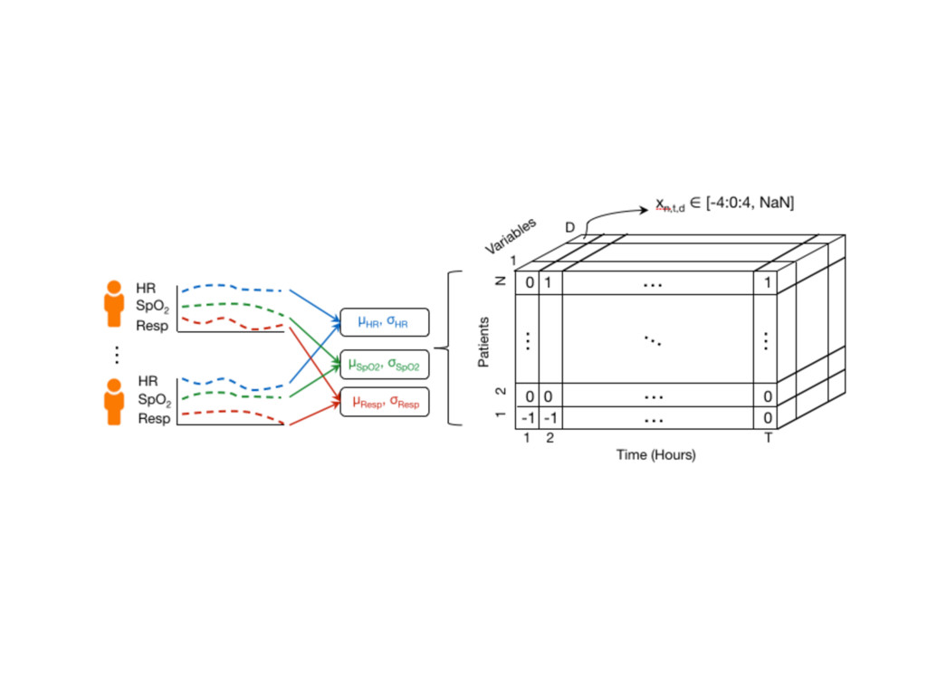
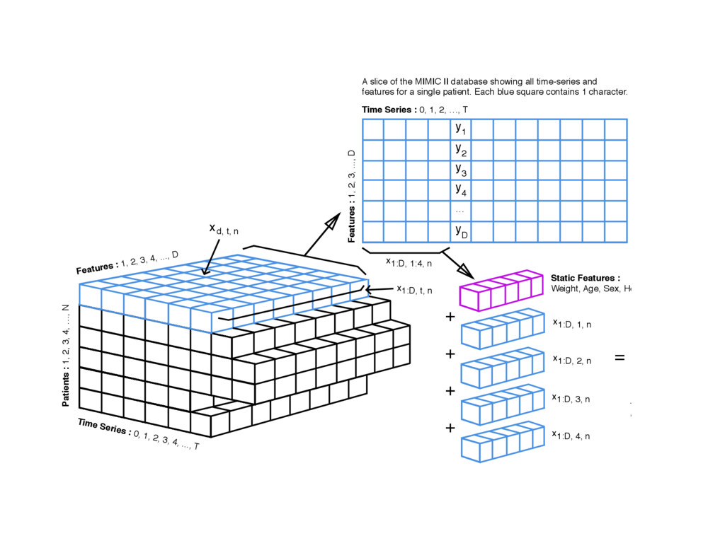
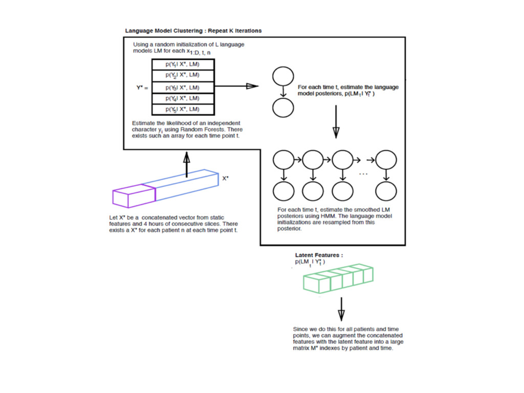
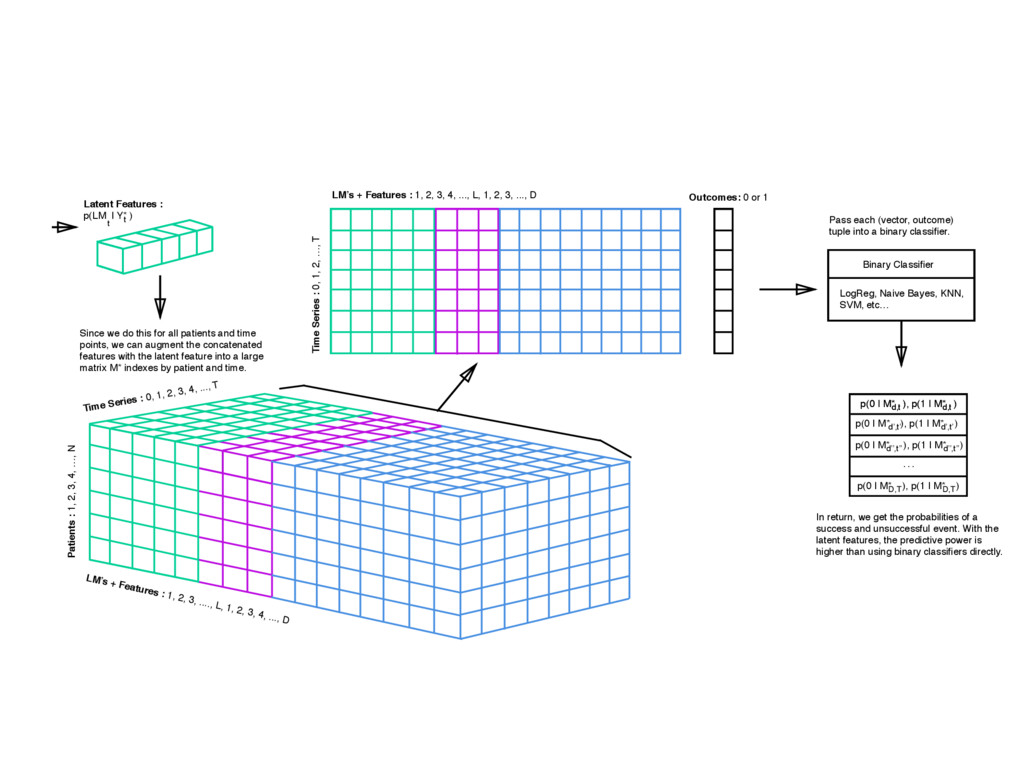
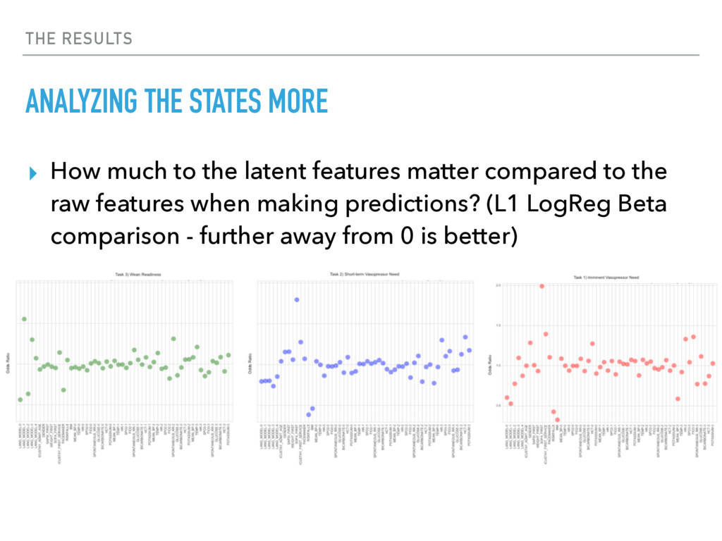
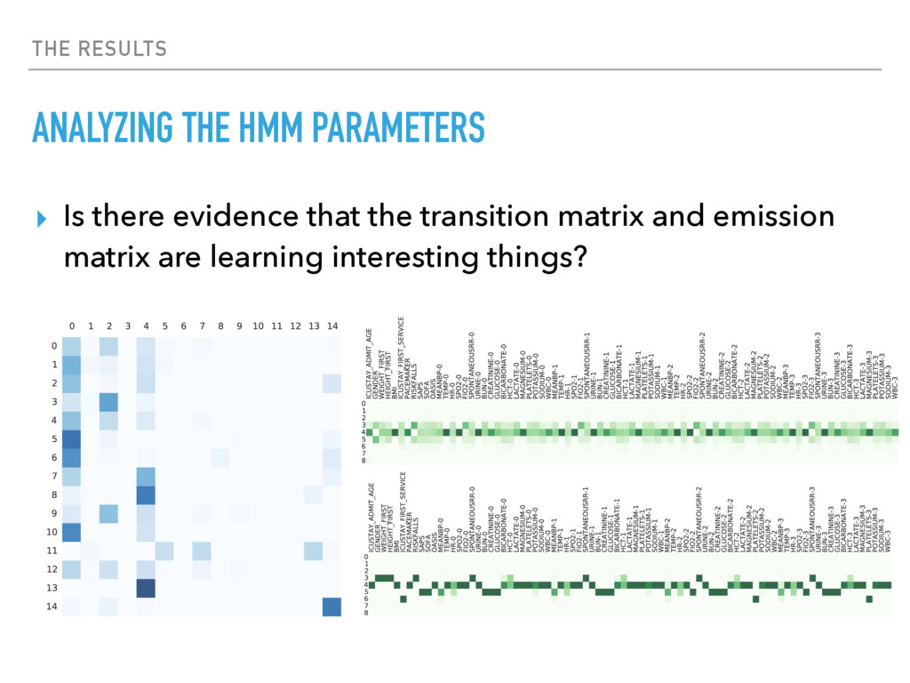
22. Patients : 1, 2, 3, 4, …, N Time Series : 0, 1, 2, 3, 4, ..., T LM’s + Features : 1, 2, 3, ...., L, 1, 2, 3, 4, ..., D Latent Features : p(LM | Y* ) Since we do this for all patients and time points, we can augment the concatenated features with the latent feature into a large matrix M* indexes by patient and time. Pass each (vector, outcome) tuple into a binary classifier. In return, we get the probabilities of a success and unsuccessful event. With the latent features, the predictive power is higher than using binary classifiers directly. age age t t el Time Series : 0, 1, 2, …, T LM’s + Features : 1, 2, 3, 4, ..., L, 1, 2, 3, ..., D Outcomes: 0 or 1 Binary Classifier LogReg, Naive Bayes, KNN, SVM, etc… … p(0 | M* ), p(1 | M* ) d,t d,t p(0 | M* ), p(1 | M* ) d’,t’ d’,t’ p(0 | M* ), p(1 | M* ) d’’,t’’ d’’,t’’ p(0 | M* ), p(1 | M* ) D,T D,T p(0 | M* ), p(1 | M* ) d,t d,t
23. THE MODEL PREDICTION TASKS ‣ Gapped intervention onset uses data from a to predict onset in c. ‣ Un-gapped intervention onset uses data from a to predict onset in b. ‣ Intervention weaning uses data from d to predict weans in e.
24. IMPLEMENTATION SPECIFICS DOING THINGS IN REASONABLE TIME ▸ Parallelized by number of states. So if you want to learn 50 states, use up to 50 nodes. ▸ Learning by batches. ▸ Warm start the same random forest across batches ▸ Loop through batches and add up probabilities from random forests before normalizing. ▸ Add counts for updating the emission & transition matrix for HMM
25. THE RESULTS RESULTS IN VASOPRESSOR ONSET PREDICTION • Benchmark to Fialho et al. (2013) using 22 features derived from physiological signals and 3 static features. • AUC of 0.79 for 2 hour gapped prediction (compared with our 0.88)
26. THE RESULTS RESULTS IN VASOPRESSOR WEANING PREDICTION Raw Features: AUC 0.67 (0.008) SSAM Features: AUC 0.63 (0.021) Raw+SSAM: AUC 0.71 (0.005) ‣ Hug (2009) used manual engineering of 438 features on 3,916 patients ‣ General model (RAS) - 0.727 AUC ‣ Targeted model (PWLM) - 0.82 AUC ‣ Patients are often left on interventions 
 longer than necessary. ‣ Extended interventions can be costly 
 and detrimental to patient health.1
28. THE RESULTS COULD WEANING HAVE BEEN DONE EARLIER?
30. THE RESULTS ANALYZING THE STATES ▸ What is the distribution of the states in those patients we are very confident will succeed in weaning and those who we are confident will not?
31. THE RESULTS ANALYZING THE STATES MORE ▸ How much to the latent features matter compared to the raw features when making predictions? (L1 LogReg Beta comparison - further away from 0 is better)
32. THE RESULTS ANALYZING THE HMM PARAMETERS ▸ Is there evidence that the transition matrix and emission matrix are learning interesting things?
33. IMPROVEMENTS HOW TO DO BETTER?
34. CURRENT WORK SAME DESIGN; DIFFERENT OUTCOMES ▸ Nothing about vasopressors is special. We can use any outcome that is related to the patient’s stay in the ICU. Here’s some I am looking at now. ▸ Vasopressor, red blood cell fusion, fresh frozen plasma fusion, platelet fusion, ventilation, mortality ▸ Results coming soon! ▸ Mortality does well! I need to run more but >0.90 AUC.
35. CURRENT WORK DIMENSIONALITY REDUCTION PRIOR TO LEARNING ▸ Concatenating 4 hours of continuous features along with the static features was to try to capture time-based relationships but maybe too much. ▸ PCA or auto-encoding prior to training.
36. CURRENT WORK CONTINUOUS VERSUS DISCRETE ▸ I z-scored the data but no reason to actually limit SSAM to the discrete space. ▸ Coded up a non-discrete version. ▸ Now creating bigram (<word, word>, word) tuples but now all words are both in R^{n}. ▸ Most things stay the same but I can’t use a random forest or Naive Bayes anymore!
37. CURRENT WORK SHALLOW NEURAL NET TO REPLACE RANDOM FOREST ▸ So use a neural network. No need to go deep. ▸ 2 dense layers (1024 hu, 256 hu), rectified linear activations, dropout, batch normalized, weight regularization, MSE loss, ADAM optimization, 25 epochs. ▸ But… because things are continuous, you can’t get probabilities of each possible output straight from the NN like before…
38. CURRENT WORK GETTING PROBABILITIES FROM A SHALLOW NETWORK ▸ A little sketchy but to get probabilities, cast Gaussian distributions. ▸ Treat the known outputs (y) as the means. ▸ This is a vector of length |features|. ▸ Standard deviation = standard deviation of predicted outputs (y_hat) per feature. ▸ Per feature, get probability of seeing the predicted value in the Gaussian distribution centered from the known output for this feature and the calculated std.
39. WORD 1 WORD 2 PREDICTED WORD 2 NN K=1 NN K=2 NN K=3 NN K=4 NN K=5 NN K=6 NN K=7 NN K=8 std
40. OTHER MODELS AUTOENCODERS / DEEP AUTOENCODERS ▸ Another way of learning latent features from the data. ▸ Seemed to have success in this paper: ▸ Miotto, Riccardo, et al. "Deep Patient: An Unsupervised Representation to Predict the Future of Patients from the Electronic Health Records." Scientific Reports 6 (2016): 26094. ▸ Learning a general purpose patient representation from a 3 layer stack of denoting auto-encoders. Applied to diabetes, schizophrenia, cancer, 78 other diseases.
41. OTHER MODELS LSTMS / BI-LSTM ▸ The LSTM we tried didn’t do so well. It couldn’t seem to pick up on anything. Feeding it time-series data per patient (reinitializing memory per patient) ▸ I tried tuning hyper parameters a lot, editing the input structure, but to no avail. ▸ Could be due my poor training. ▸ Better idea: forward and backward LSTMs.
42. BIG THANKS LOTS OF CREDIT GOES TO… ▸ Marzyeh Ghassemi (MIT) ▸ Finale Doshi-Velez (Harvard) ▸ Peter Solovitz (MIT) THANKS FOR LISTENING! QUESTIONS?