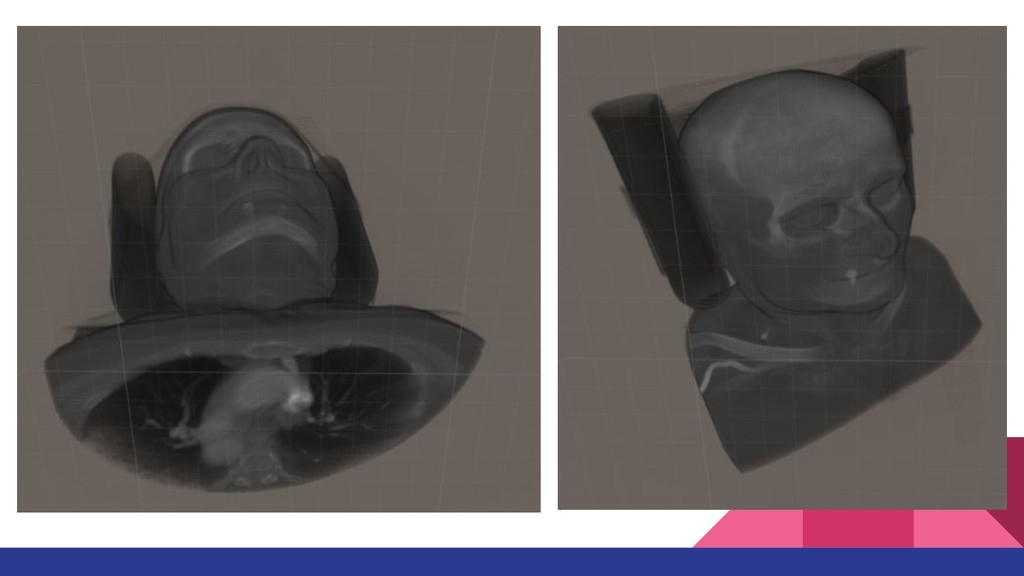
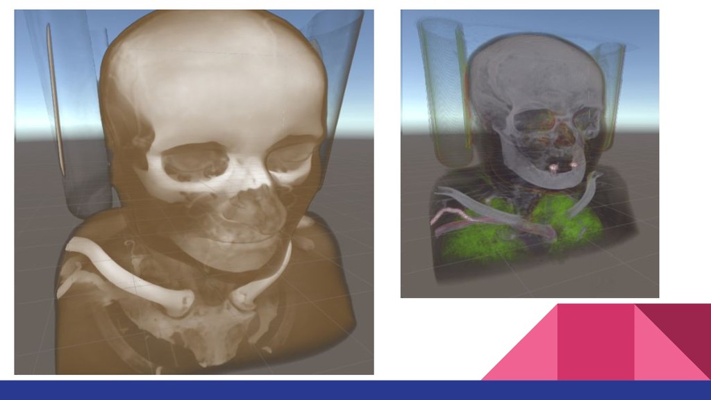
Volume Rendering in Unity3D

Volume rendering 3D volume data (medical CT scans) in Unity3D.
Covering the following topics:
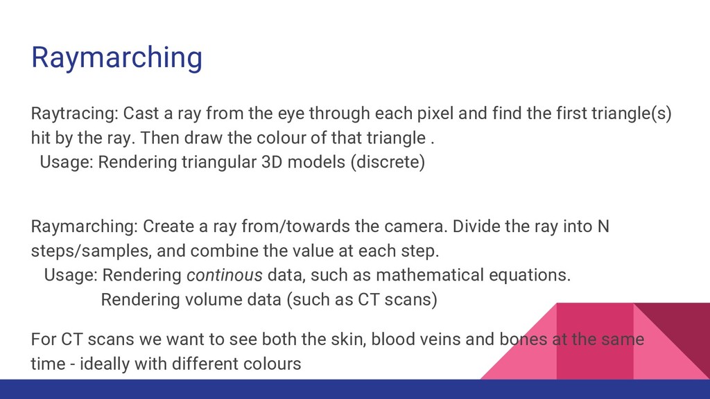
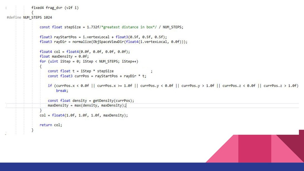
- Raymarching
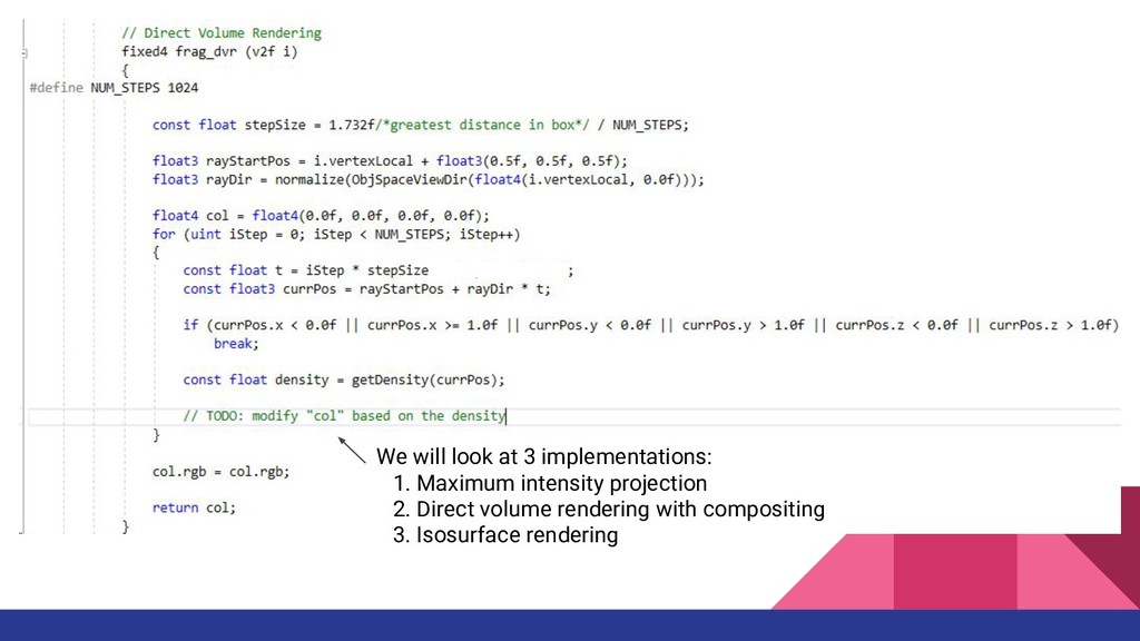
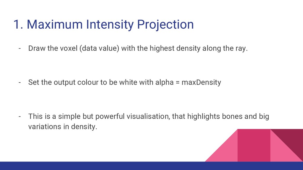
- Maximum Intensity Projection
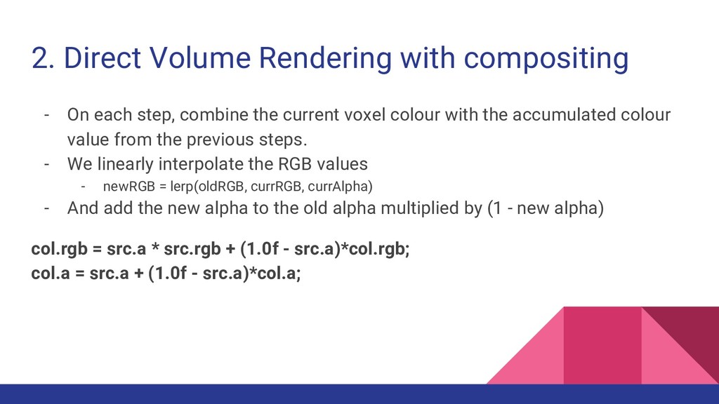
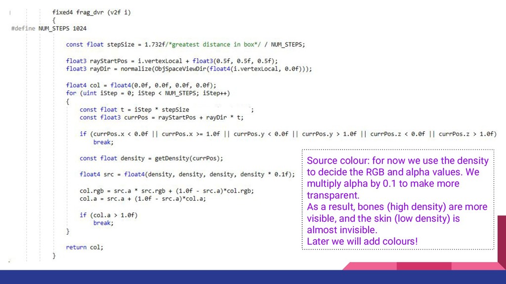
- Direct Volume Rendering with compositing
- Isosurface rendering
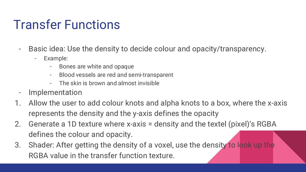
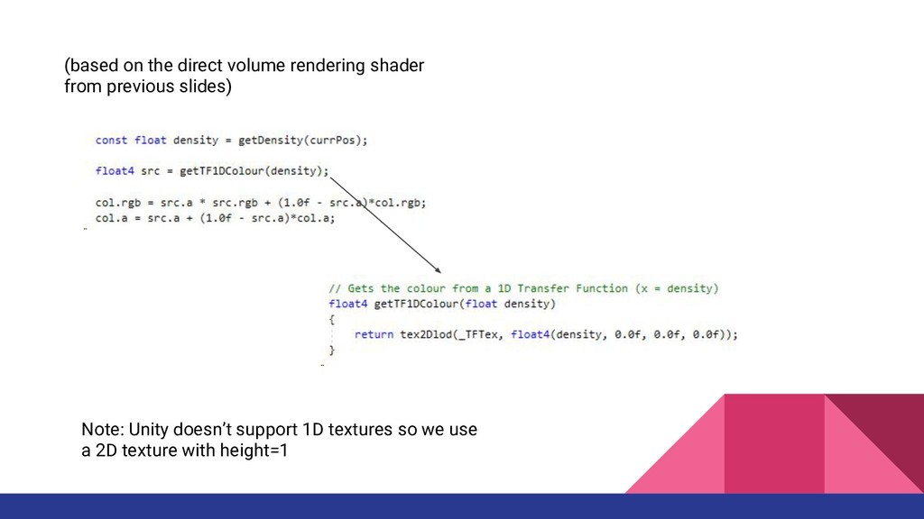
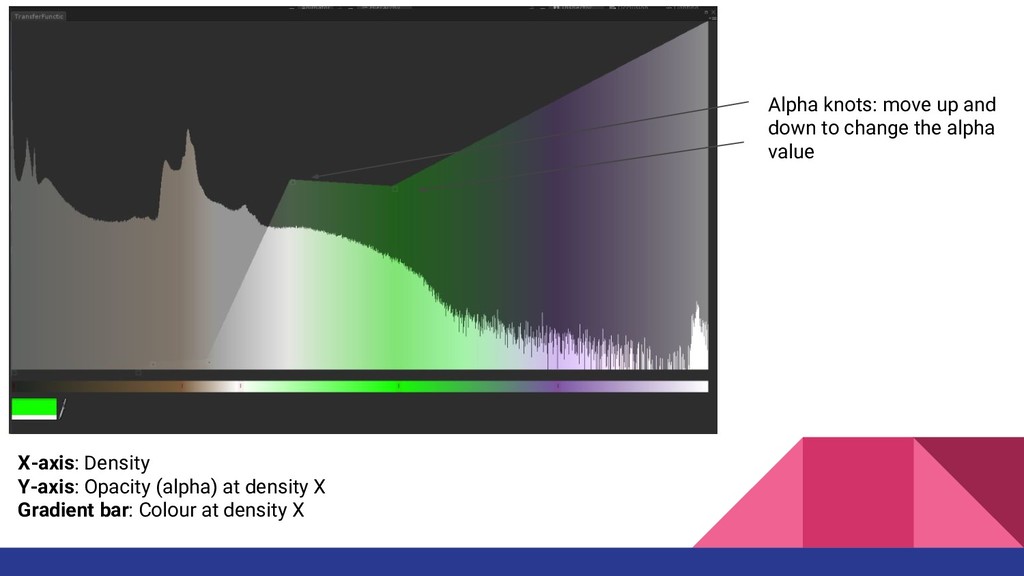
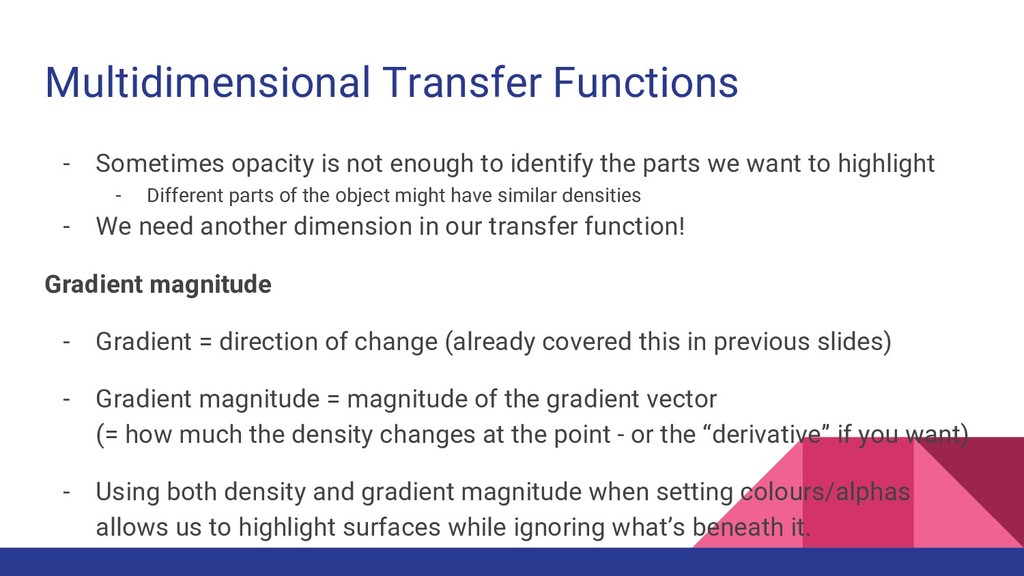
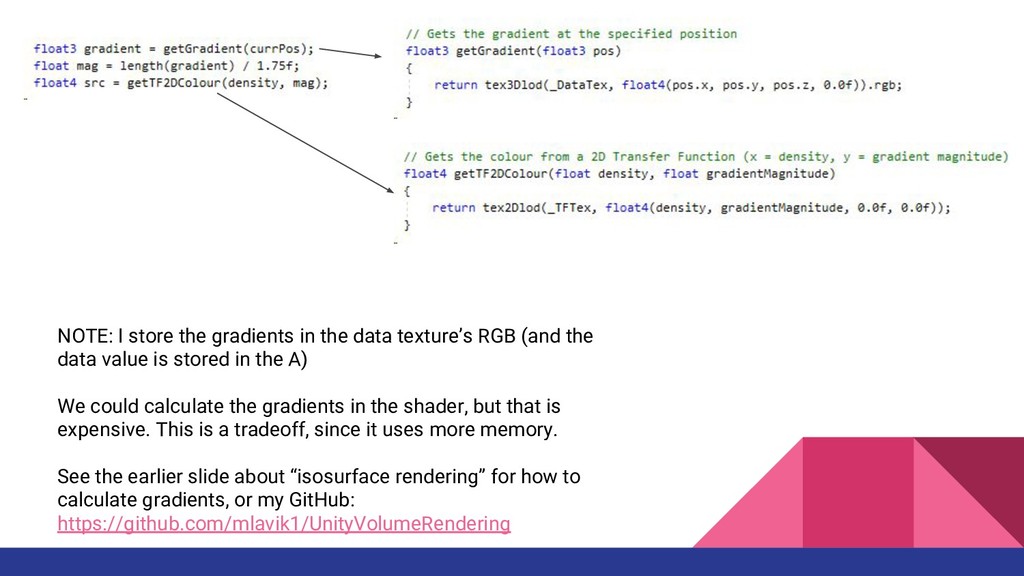
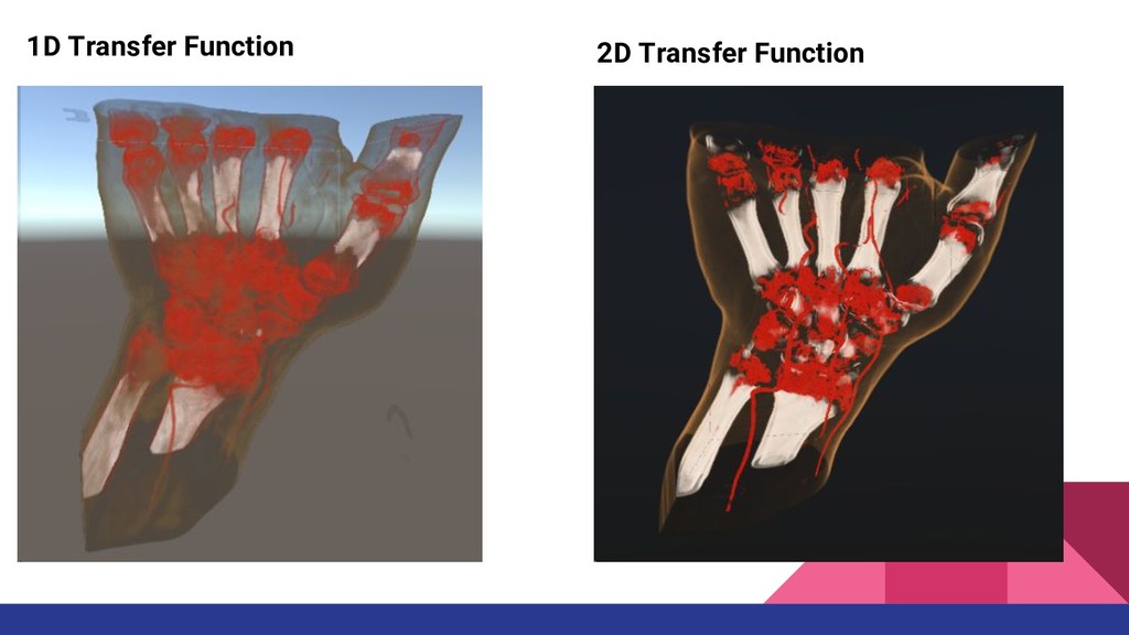
- Transfer functions
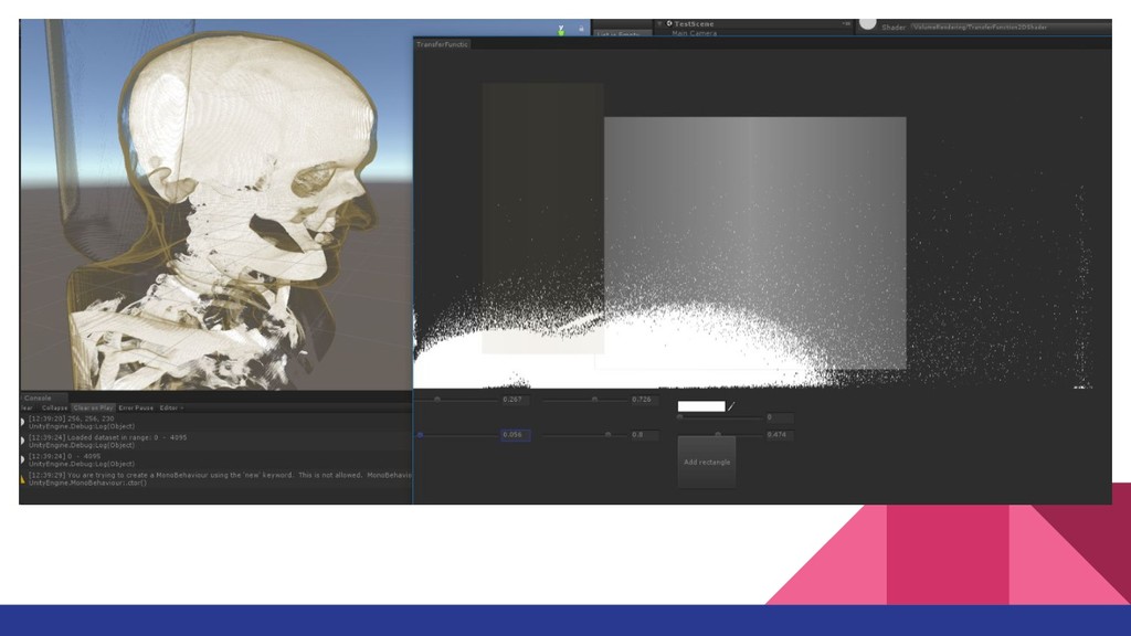
- 2D Transfer Functions
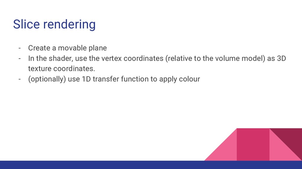
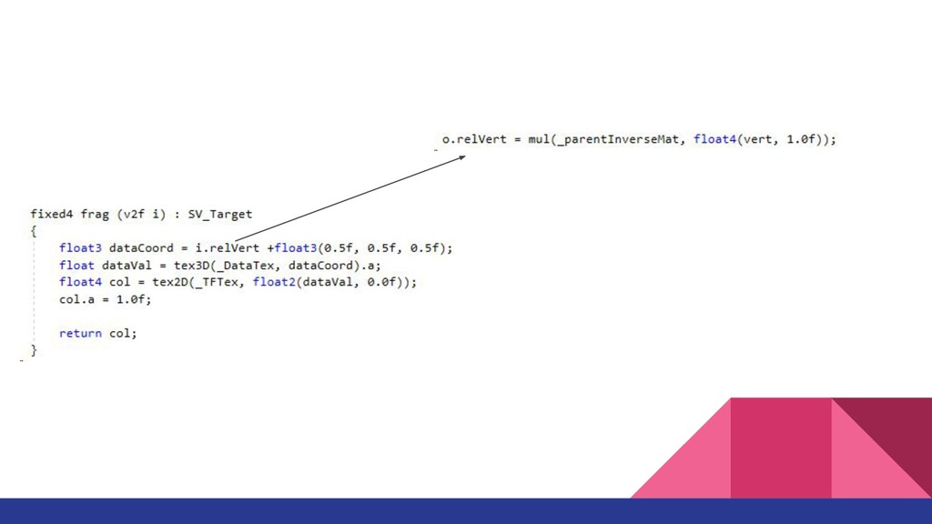
- Slice rendering

Source code here: https://github.com/mlavik1/UnityVolumeRendering

From an internal presentation I had at our company.

Transcript

1. Volume Rendering In Unity3D Matias Lavik
2. The presentation - An introduction to volume rendering of medical 3D volume data. - Based on my hobby-project: https://github.com/mlavik1/UnityVolumeRendering (still WIP) - What we will cover: - Raymarching volume data - Techniques for volume rendering: Direct volume rendering with compositing, maximum intensity projection, isosurface rendering - Diffuse lighting - Transfer functions - Multidimensional transfer functions
3. The data - We use 3D voxel data from a medical CT scan. - The value of each data point represents the density. - The data is read from a file and stored in a 3D texture - The data fits nicely into a box, so we render a box (we only draw the back faces) and use raymarching to fetch the densities of each visible voxel inside the box.
4. (above illustration by: Klaus D Tönnies https://www.researchgate.net/figure/3D-volume-d ata-representation_fig1_238687132 )
5. Raymarching Raytracing: Cast a ray from the eye through each pixel and find the first triangle(s) hit by the ray. Then draw the colour of that triangle . Usage: Rendering triangular 3D models (discrete) Raymarching: Create a ray from/towards the camera. Divide the ray into N steps/samples, and combine the value at each step. Usage: Rendering continous data, such as mathematical equations. Rendering volume data (such as CT scans) For CT scans we want to see both the skin, blood veins and bones at the same time - ideally with different colours
6. Raymarching the data 1. Draw the back-faces of a box 2. For each vertex: 2.1. Set startPos as the vertex local position 2.2. Set rayDir as the direction towards the eye (in model space) 2.3. Divide the ray into N steps/samples 2.4. For each step (starting at startPos moving along rayDir) 2.4.1. Get the density: use currentPos as a texture coordinate and fetch the value from the 3D texture 2.4.2. ??? (use the density to decide the output colour of the fragment/pixel)
7. startPos: we start from here rayDir: direction towards the eye n steps: we get the density (data value) at each step we stop at the border of the box
8. We will look at 3 implementations: 1. Maximum intensity projection 2. Direct volume rendering with compositing 3. Isosurface rendering
9. 1. Maximum Intensity Projection - Draw the voxel (data value) with the highest density along the ray. - Set the output colour to be white with alpha = maxDensity - This is a simple but powerful visualisation, that highlights bones and big variations in density.
11. Result
12. 2. Direct Volume Rendering with compositing - On each step, combine the current voxel colour with the accumulated colour value from the previous steps. - We linearly interpolate the RGB values - newRGB = lerp(oldRGB, currRGB, currAlpha) - And add the new alpha to the old alpha multiplied by (1 - new alpha) col.rgb = src.a * src.rgb + (1.0f - src.a)*col.rgb; col.a = src.a + (1.0f - src.a)*col.a;
13. Source colour: for now we use the density to decide the RGB and alpha values. We multiply alpha by 0.1 to make more transparent. As a result, bones (high density) are more visible, and the skin (low density) is almost invisible. Later we will add colours!
15. 3. Isosurface Rendering - Draw the first voxel (data value) with a density higher than some threshold. - Now we need to start raymarching at the eye (or ideally at the point where the ray hits the front face of the box) and move away from the eye. - When we hit a voxel with density > threshold we stop, and use that density -
16. Lighting - Since we are rendering the surfaces only, we need light reflection to make it look good. Diffuse reflection: Light intensity is decided by the angle between the direction to the light source and the surface normal (θ), and a diffuse constant (Kd - we can set it to 1). Id = Kd · cos(θ) When l and n are normalised, we have: cos(θ) = dot(n, l) Id = Kd · dot(n, l)
17. How do we get the normal? - Since we are working with 3D voxels and not triangles, getting the normal requires some extra work. Solution: Use the gradient Gradient = direction of change Compare the neighbour data values in each axis When the data values decrease towards the right (positive X-axis), the normal will point to the right
18. You might want to use another lighting calculation, such as Phong (which includes specular reflection as well). NOTE: Here we use a transfer function to decide colour. (see next slides) (Note: we now add a random offset to the ray start position, to improve the sample artifacts.)
19. Without lighting With lighting
20. With Transfer Function (see next slides)
21. Transfer Functions - Basic idea: Use the density to decide colour and opacity/transparency. - Example: - Bones are white and opaque - Blood vessels are red and semi-transparent - The skin is brown and almost invisible - Implementation 1. Allow the user to add colour knots and alpha knots to a box, where the x-axis represents the density and the y-axis defines the opacity 2. Generate a 1D texture where x-axis = density and the textel (pixel)’s RGBA defines the colour and opacity. 3. Shader: After getting the density of a voxel, use the density to look up the RGBA value in the transfer function texture.
22. (based on the direct volume rendering shader from previous slides) Note: Unity doesn’t support 1D textures so we use a 2D texture with height=1
23. X-axis: Density Y-axis: Opacity (alpha) at density X Gradient bar: Colour at density X Alpha knots: move up and down to change the alpha value
25. Multidimensional Transfer Functions - Sometimes opacity is not enough to identify the parts we want to highlight - Different parts of the object might have similar densities - We need another dimension in our transfer function! Gradient magnitude - Gradient = direction of change (already covered this in previous slides) - Gradient magnitude = magnitude of the gradient vector (= how much the density changes at the point - or the “derivative” if you want) - Using both density and gradient magnitude when setting colours/alphas allows us to highlight surfaces while ignoring what’s beneath it.
26. NOTE: I store the gradients in the data texture’s RGB (and the data value is stored in the A) We could calculate the gradients in the shader, but that is expensive. This is a tradeoff, since it uses more memory. See the earlier slide about “isosurface rendering” for how to calculate gradients, or my GitHub: https://github.com/mlavik1/UnityVolumeRendering
27. 1D Transfer Function 2D Transfer Function
29. Slice rendering - Create a movable plane - In the shader, use the vertex coordinates (relative to the volume model) as 3D texture coordinates. - (optionally) use 1D transfer function to apply colour
32. References / credits - ImageVis3D - Some of the GUI are heavily inspired by ImageVis3D - Get ImageVis3D here: http://www.sci.utah.edu/software/imagevis3d.html - Marcelo Lima - Marcelo presented his implementation of isosurface rendering during his assignment presentation for the Visualisation course at the University of Bergen. - See his amazing project here: https://github.com/m-lima/KATscans - Thanks to Stefan Bruckner and Helwig Hauser who taught me CG and visualisation at the University of Bergen.