Test Project

A test!

Transcript

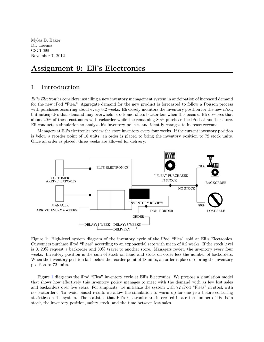
1. Myles D. Baker Dr. Leemis CSCI 698 November 7, 2012 Assignment 9: Eli’s Electronics 1 Introduction Eli’s Electronics considers installing a new inventory management system in anticipation of increased demand for the new iPod “Flea.” Aggregate demand for the new product is forecasted to follow a Poisson process with purchases occurring about every 0.2 weeks. Eli closely monitors the inventory position for the new iPod, but anticipates that demand may overwhelm stock and offers backorders when this occurs. Eli observes that about 20% of these customers will backorder while the remaining 80% purchase the iPod at another store. Eli conducts a simulation to analyze his inventory policies and identify changes to increase revenue. Managers at Eli’s electronics review the store inventory every four weeks. If the current inventory position is below a reorder point of 18 units, an order is placed to bring the inventory position to 72 stock units. Once an order is placed, three weeks are allowed for delivery. ELI’S ELECTRONICS MANAGER INVENTORY REVIEW DON’T ORDER ORDER DELAY: 3 WEEKS DELIVERY DELAY: 1 WEEK CUSTOMER ARRIVE: EXPO(0.2) ARRIVE: EVERY 4 WEEKS 20% 80% NO STOCK IN STOCK ’’FLEA’’ PURCHASED BACKORDER LOST SALE Figure 1: High-level system diagram of the inventory cycle of the iPod “Flea” sold at Eli’s Electronics. Customers purchase iPod “Fleas” according to an exponential rate with mean of 0.2 weeks. If the stock level is 0, 20% request a backorder and 80% travel to another store. Managers review the inventory every four weeks. Inventory position is the sum of stock on hand and stock on order less the number of backorders. When the inventory position falls below the reorder point of 18 units, an order is placed to bring the inventory position to 72 units. Figure 1 diagrams the iPod “Flea” inventory cycle at Eli’s Electronics. We propose a simulation model that shows how effectively this inventory policy manages to meet with the demand with as few lost sales and backorders over five years. For simplicity, we initialize the system with 72 iPod “Fleas” in stock with no backorders. To avoid biased results we allow the simulation to warm up for one year before collecting statistics on the system. The statistics that Eli’s Electronics are interested in are the number of iPods in stock, the inventory position, safety stock, and the time between lost sales.
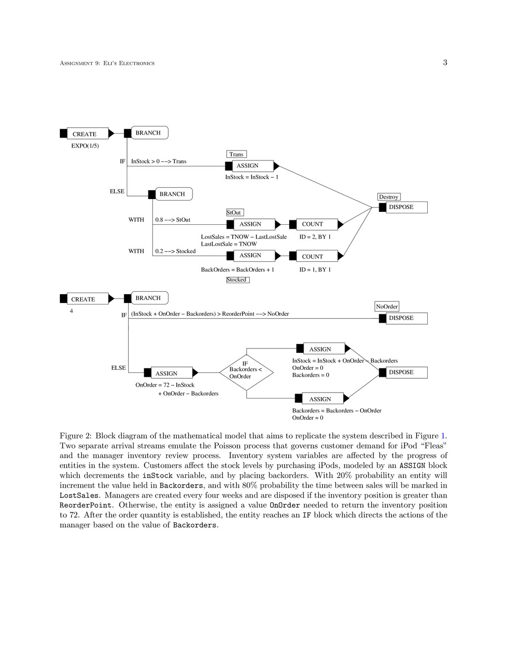
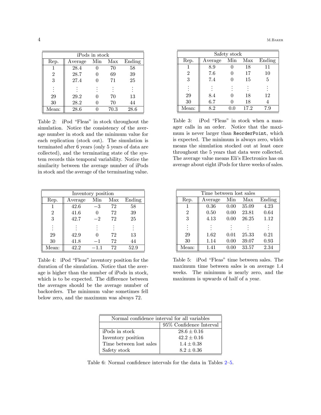
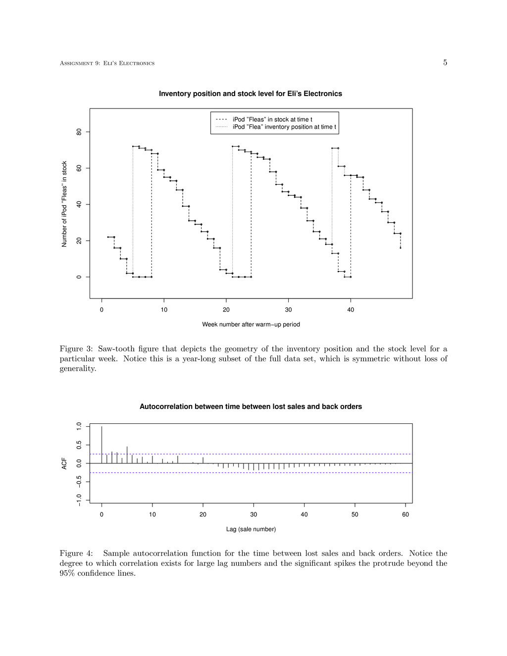
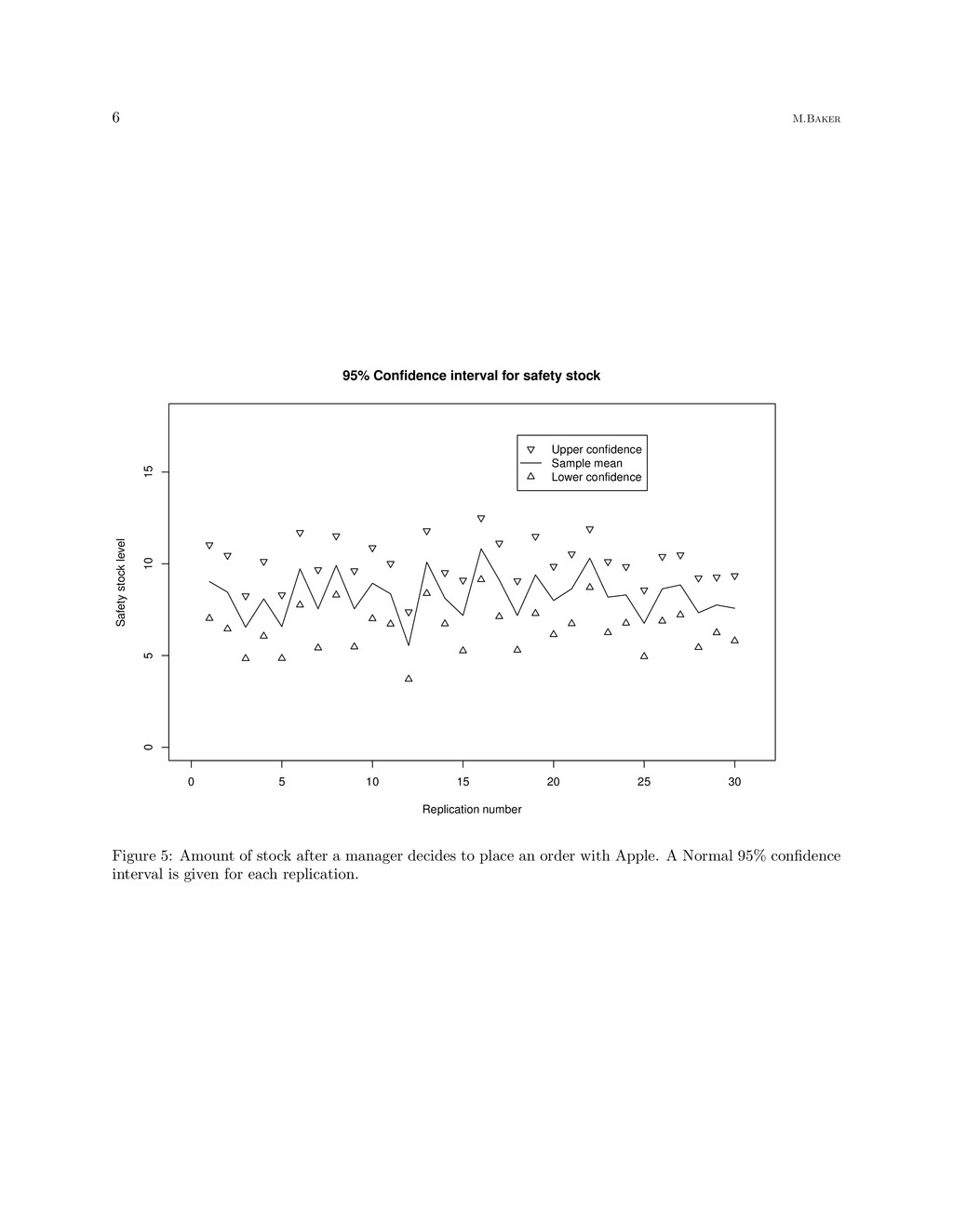
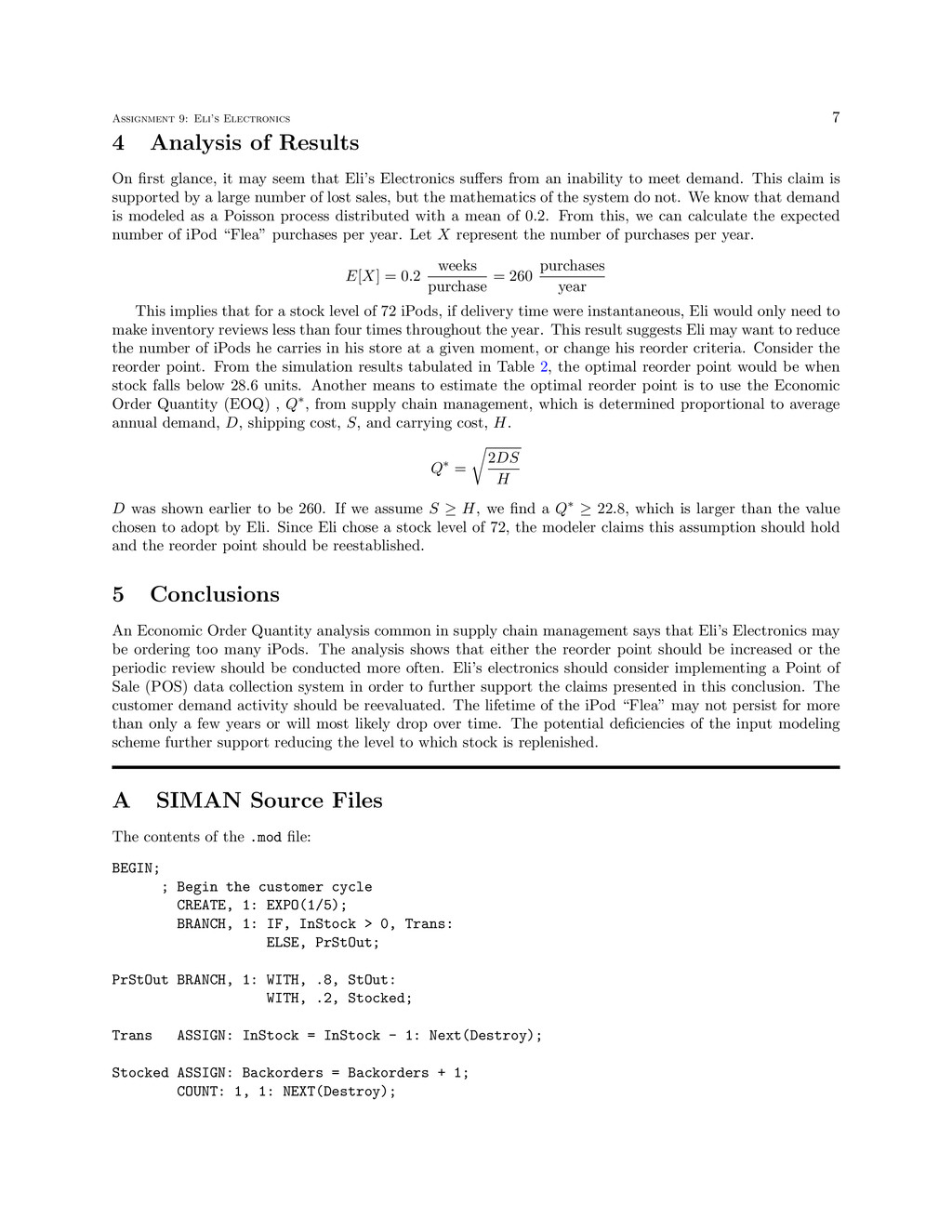
2. 2 M.Baker 2 Model Description SIMAN is used to model the system. For this system we have the following assumptions: 1. The warm up period allows for the system to achieve a steady-state. 2. Seasonality is not accounted for. 3. The system parameters may be modified. We desire an extensible model. 4. The service component of Eli’s Electronics does not affect any customers purchase decision. 5. Managers review the inventory level at exactly the four week mark. Furthermore, deliveries take exactly three weeks and Apple always can always fully meet Eli’s stock requests. 2.1 Block Diagram The system diagramed in Figure 1 easily translates into the SIMAN model depicted in Figure 2. The most striking difference between this and other SIMAN models is the absence of a QUEUE-SEIZE-DELAY-RELEASE chain. In many ways, this Monte Carlo simulation could be implemented in other languages like R because it doesn’t utilize features unique to SIMAN. This model destroys managers based on a branching condition rather than cycling one manager in a DELAY condition. 2.2 SIMAN Variables All SIMAN variables are initialized to 0, except for InStock and ReorderPoint, which are set to 72 and 18, respectively. Table 1 summarizes the meanings of the different variables used during the simulation. Variable name Meaning Initial value InStock Current number of iPods in stock 72 ReorderPoint Number governing ordering decision during periodic review 18 OnOrder Current number of iPods in stock 0 LostSales Time between lost sale 0 LastLostSale Time recorded during the last lost sale 0 Backorders Number of backorders 0 SafetyStock iPods in stock when an order is placed 0 Table 1: Summary of variables 2.3 SIMAN Attributes and Queues No SIMAN attributes or queues are used in this model. 3 Presentation of Results In this section the results of the simulation are presented and analyzed. In order to conduct an analysis we collect data for the number of iPods in stock, on order, and backordered. The time between lost sales is recorded . Since the simulation is run thirty times, we can aggregate results over all runs. However, for simplicity of this analysis, we present summary data in Tables 2–6 and Figures 3–5. In Table 2 we present the stock level throughout the simulation. Table 3 shows the level of safety stock and is depicted in Figure 5. Table 4 displays the inventory position and combined with Table 2 has a saw- tooth depiction in Figure 3. Table 5 shows the time between lost sales. Table 6 contains calculated Normal 95% confidence intervals for all of the data contained in Tables 2–5, and the confidence interval for safety stock is presented in Figure 5. Figure 4 shows the relationship between backorders and lost sales.
3. Assignment 9: Eli’s Electronics 3 DISPOSE BRANCH BRANCH DISPOSE BRANCH ASSIGN ASSIGN ASSIGN COUNT CREATE COUNT EXPO(1/5) InStock > 0 −−> Trans WITH 0.8 −−> StOut 0.2 −−> Stocked ID = 2, BY 1 ID = 1, BY 1 ASSIGN DISPOSE ASSIGN ASSIGN CREATE InStock = InStock + OnOrder − Backorders OnOrder = 0 Backorders = 0 Backorders = Backorders − OnOrder OnOrder = 0 IF ELSE InStock = InStock − 1 Destroy Trans WITH LostSales = TNOW − LastLostSale LastLostSale = TNOW BackOrders = BackOrders + 1 StOut Stocked IF (InStock + OnOrder − Backorders) > ReorderPoint −−> NoOrder NoOrder ELSE OnOrder = 72 − InStock + OnOrder − Backorders IF Backorders < OnOrder 4 Figure 2: Block diagram of the mathematical model that aims to replicate the system described in Figure 1. Two separate arrival streams emulate the Poisson process that governs customer demand for iPod “Fleas” and the manager inventory review process. Inventory system variables are affected by the progress of entities in the system. Customers affect the stock levels by purchasing iPods, modeled by an ASSIGN block which decrements the inStock variable, and by placing backorders. With 20% probability an entity will increment the value held in Backorders, and with 80% probability the time between sales will be marked in LostSales. Managers are created every four weeks and are disposed if the inventory position is greater than ReorderPoint. Otherwise, the entity is assigned a value OnOrder needed to return the inventory position to 72. After the order quantity is established, the entity reaches an IF block which directs the actions of the manager based on the value of Backorders.
4. 4 M.Baker iPods in stock Rep. Average Min Max Ending 1 28.4 0 70 58 2 28.7 0 69 39 3 27.4 0 71 25 . . . . . . . . . . . . . . . 29 29.2 0 70 13 30 28.2 0 70 44 Mean: 28.6 0 70.3 28.6 Table 2: iPod “Fleas” in stock throughout the simulation. Notice the consistency of the aver- age number in stock and the minimum value for each replication (stock out). The simulation is terminated after 6 years (only 5 years of data are collected), and the terminating state of the sys- tem records this temporal variability. Notice the similarity between the average number of iPods in stock and the average of the terminating value. Safety stock Rep. Average Min Max Ending 1 8.9 0 18 11 2 7.6 0 17 10 3 7.4 0 15 5 . . . . . . . . . . . . . . . 29 8.4 0 18 12 30 6.7 0 18 4 Mean: 8.2 0.0 17.2 7.9 Table 3: iPod “Fleas” in stock when a man- ager calls in an order. Notice that the maxi- mum is never larger than ReorderPoint, which is expected. The minimum is always zero, which means the simulation stocked out at least once throughout the 5 years that data were collected. The average value means Eli’s Electronics has on average about eight iPods for three weeks of sales. Inventory position Rep. Average Min Max Ending 1 42.6 −3 72 58 2 41.6 0 72 39 3 42.7 −2 72 25 . . . . . . . . . . . . . . . 29 42.9 0 72 13 30 41.8 −1 72 44 Mean: 42.2 −1.1 72 52.9 Table 4: iPod “Fleas” inventory position for the duration of the simulation. Notice that the aver- age is higher than the number of iPods in stock, which is to be expected. The difference between the averages should be the average number of backorders. The minimum value sometimes fell below zero, and the maximum was always 72. Time between lost sales Rep. Average Min Max Ending 1 0.36 0.00 35.09 4.23 2 0.50 0.00 23.81 0.64 3 4.13 0.00 26.25 1.12 . . . . . . . . . . . . . . . 29 1.62 0.01 25.33 0.21 30 1.14 0.00 39.07 0.93 Mean: 1.41 0.00 33.57 2.34 Table 5: iPod “Fleas” time between sales. The maximum time between sales is on average 1.4 weeks. The minimum is nearly zero, and the maximum is upwards of half of a year. Normal confidence interval for all variables 95% Confidence Interval iPods in stock 28.6 ± 0.16 Inventory position 42.2 ± 0.16 Time between lost sales 1.4 ± 0.38 Safety stock 8.2 ± 0.36 Table 6: Normal confidence intervals for the data in Tables 2–5.
5. Assignment 9: Eli’s Electronics 5 0 10 20 30 40 0 20 40 60 80 Inventory position and stock level for Eli’s Electronics Week number after warm−up period Number of iPod ’’Fleas’’ in stock iPod ’’Fleas’’ in stock at time t iPod ’’Flea’’ inventory position at time t Figure 3: Saw-tooth figure that depicts the geometry of the inventory position and the stock level for a particular week. Notice this is a year-long subset of the full data set, which is symmetric without loss of generality. 0 10 20 30 40 50 60 −1.0 −0.5 0.0 0.5 1.0 Lag (sale number) ACF Autocorrelation between time between lost sales and back orders Figure 4: Sample autocorrelation function for the time between lost sales and back orders. Notice the degree to which correlation exists for large lag numbers and the significant spikes the protrude beyond the 95% confidence lines.
6. 6 M.Baker 0 5 10 15 20 25 30 0 5 10 15 95% Confidence interval for safety stock Replication number Safety stock level Upper confidence Sample mean Lower confidence Figure 5: Amount of stock after a manager decides to place an order with Apple. A Normal 95% confidence interval is given for each replication.
7. Assignment 9: Eli’s Electronics 7 4 Analysis of Results On first glance, it may seem that Eli’s Electronics suffers from an inability to meet demand. This claim is supported by a large number of lost sales, but the mathematics of the system do not. We know that demand is modeled as a Poisson process distributed with a mean of 0.2. From this, we can calculate the expected number of iPod “Flea” purchases per year. Let X represent the number of purchases per year. E[X] = 0.2 weeks purchase = 260 purchases year This implies that for a stock level of 72 iPods, if delivery time were instantaneous, Eli would only need to make inventory reviews less than four times throughout the year. This result suggests Eli may want to reduce the number of iPods he carries in his store at a given moment, or change his reorder criteria. Consider the reorder point. From the simulation results tabulated in Table 2, the optimal reorder point would be when stock falls below 28.6 units. Another means to estimate the optimal reorder point is to use the Economic Order Quantity (EOQ) , Q∗, from supply chain management, which is determined proportional to average annual demand, D, shipping cost, S, and carrying cost, H. Q∗ = 2DS H D was shown earlier to be 260. If we assume S ≥ H, we find a Q∗ ≥ 22.8, which is larger than the value chosen to adopt by Eli. Since Eli chose a stock level of 72, the modeler claims this assumption should hold and the reorder point should be reestablished. 5 Conclusions An Economic Order Quantity analysis common in supply chain management says that Eli’s Electronics may be ordering too many iPods. The analysis shows that either the reorder point should be increased or the periodic review should be conducted more often. Eli’s electronics should consider implementing a Point of Sale (POS) data collection system in order to further support the claims presented in this conclusion. The customer demand activity should be reevaluated. The lifetime of the iPod “Flea” may not persist for more than only a few years or will most likely drop over time. The potential deficiencies of the input modeling scheme further support reducing the level to which stock is replenished. A SIMAN Source Files The contents of the .mod file: BEGIN; ; Begin the customer cycle CREATE, 1: EXPO(1/5); BRANCH, 1: IF, InStock > 0, Trans: ELSE, PrStOut; PrStOut BRANCH, 1: WITH, .8, StOut: WITH, .2, Stocked; Trans ASSIGN: InStock = InStock - 1: Next(Destroy); Stocked ASSIGN: Backorders = Backorders + 1; COUNT: 1, 1: NEXT(Destroy);
8. 8 M.Baker StOut ASSIGN: LostSales = TNOW - LastLostSale: LastLostSale = TNOW; COUNT: 2, 1: NEXT(Destroy); Destroy DISPOSE; ; Reordering Cycle CREATE, 1: 4; BRANCH, 1: IF, (InStock + OnOrder - Backorders) > ReorderPoint, NoOrder: ELSE, Order; NoOrder DISPOSE; Order ASSIGN: OnOrder = 72 - (InStock + OnOrder - Backorders): SafetyStock = InStock; DELAY: 3; IF: BackOrders < OnOrder; ASSIGN: InStock = InStock + OnOrder - Backorders: OnOrder = 0: Backorders = 0; ELSE; ASSIGN: Backorders = Backorders - OnOrder: OnOrder = 0; ENDIF; DISPOSE; END; The contents of the .exp file: BEGIN; PROJECT, Elis Electronic Store, Myles Baker; VARIABLES: InStock, 72: OnOrder, 0: Backorders, 0: LostSales, 0: LastLostSale, 0: SafetyStock, 72: ReorderPoint, 18; REPLICATE, 30, 0, 312, , , 52; COUNTERS: 1, Backorders filled: 2, Lost sales; DSTATS: InStock, iPod Fleas in stock, "hw9-instock.doc": SafetyStock, iPod Fleas in stock at time of order, "hw9-safetystock.doc":
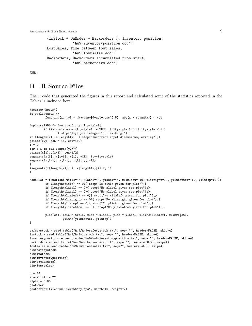
9. Assignment 9: Eli’s Electronics 9 (InStock + OnOrder - Backorders ), Inventory position, "hw9-inventoryposition.doc": LostSales, Time between lost sales, "hw9-lostsales.doc": Backorders, Backorders accumulated from start, "hw9-backorders.doc"; END; B R Source Files The R code that generated the figures in this report and calculated some of the statistics reported in the Tables is included here. #source("hw1.r") is.wholenumber <- function(x, tol = .Machine$double.eps^0.5) abs(x - round(x)) < tol EmpiricalADD <- function(x, y, ltystyle){ if (is.wholenumber(ltystyle) != TRUE || ltystyle > 6 || ltystyle < 1 ) { stop("ltystyle integer 1-6, exiting.");} if (length(x) != length(y)) { stop("Incorrect input dimensions, exiting");} points(x,y, pch = 16, cex=1/2) i = 0 for ( i in c(2:length(y))){ points(x[i],y[i-1], cex=1/2) segments(x[i], y[i-1], x[i], y[i], lty=ltystyle) segments(x[i-1], y[i-1], x[i], y[i-1]) } #segments(x[length(x)], 1, x[length(x)]*1.2, 1) } MakePlot = function( title="", xlabel="", ylabel="", xlimleft=-10, xlimright=10, ylimbottom=-10, ylimtop=10 ){ if (length(title) == 0){ stop("No title given for plot");} if (length(xlabel) == 0){ stop("No xlabel given for plot");} if (length(ylabel) == 0){ stop("No ylabel given for plot");} if (length(xlimleft) == 0){ stop("No xlimleft given for plot");} if (length(xlimright) == 0){ stop("No xlimright given for plot");} if (length(ylimtop) == 0){ stop("No ylimtop given for plot");} if (length(ylimbottom) == 0){ stop("No ylimbottom given for plot");} plot(c(), main = title, xlab = xlabel, ylab = ylabel, xlim=c(xlimleft, xlimright), ylim=c(ylimbottom, ylimtop)) } safetystock = read.table("hw9/hw9-safetystock.txt", sep= "", header=FALSE, skip=4) instock = read.table("hw9/hw9-instock.txt", sep= "", header=FALSE, skip=4) inventoryposition = read.table("hw9/hw9-inventoryposition.txt", sep= "", header=FALSE, skip=4) backorders = read.table("hw9/hw9-backorders.txt", sep= "", header=FALSE, skip=4) lostsales = read.table("hw9/hw9-lostsales.txt", sep="", header=FALSE, skip=4) dim(safetystock) dim(instock) dim(inventoryposition) dim(backorders) dim(lostsales) n = 48 stocklimit = 72 alpha = 0.05 plot.new postscript(file="hw9-inventory.eps", width=10, height=7)
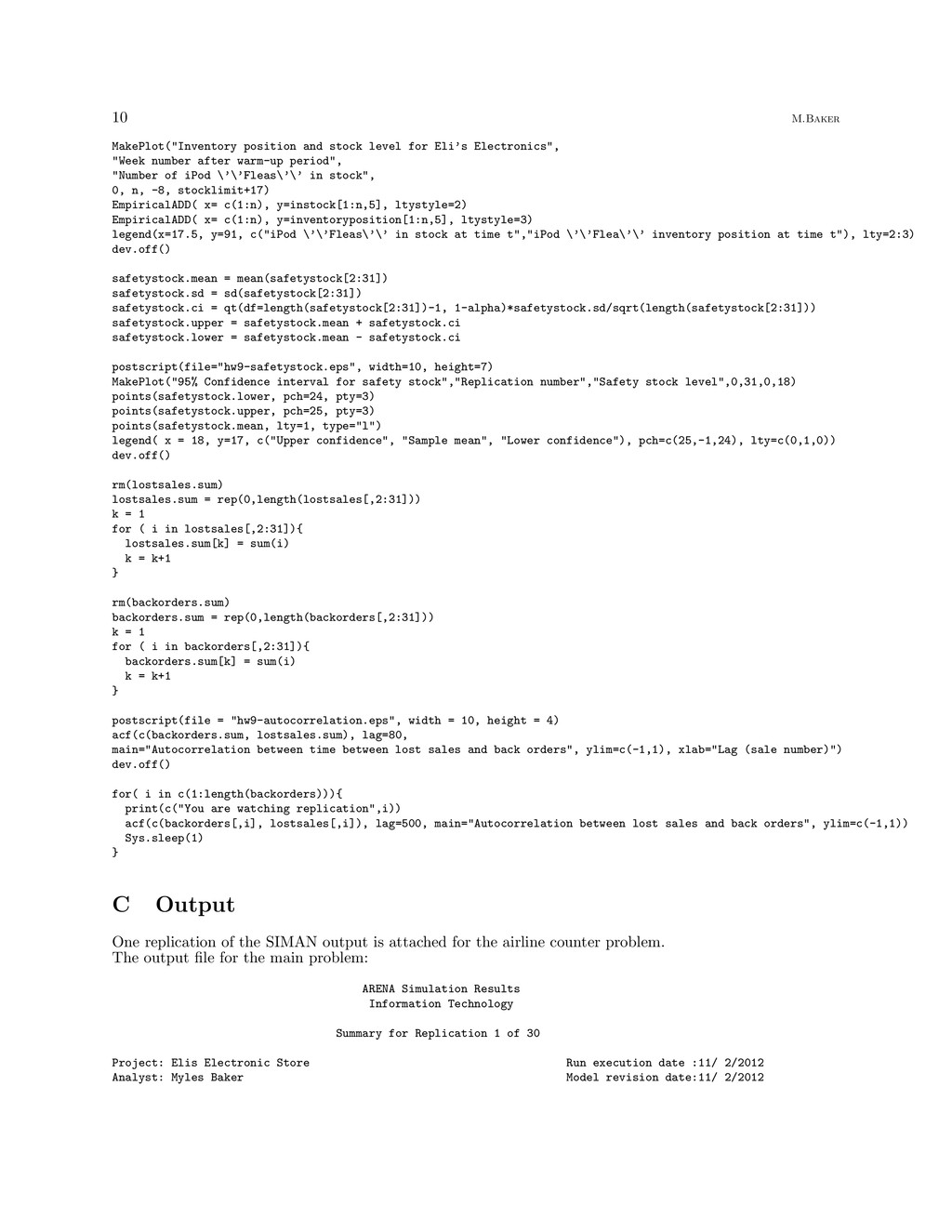
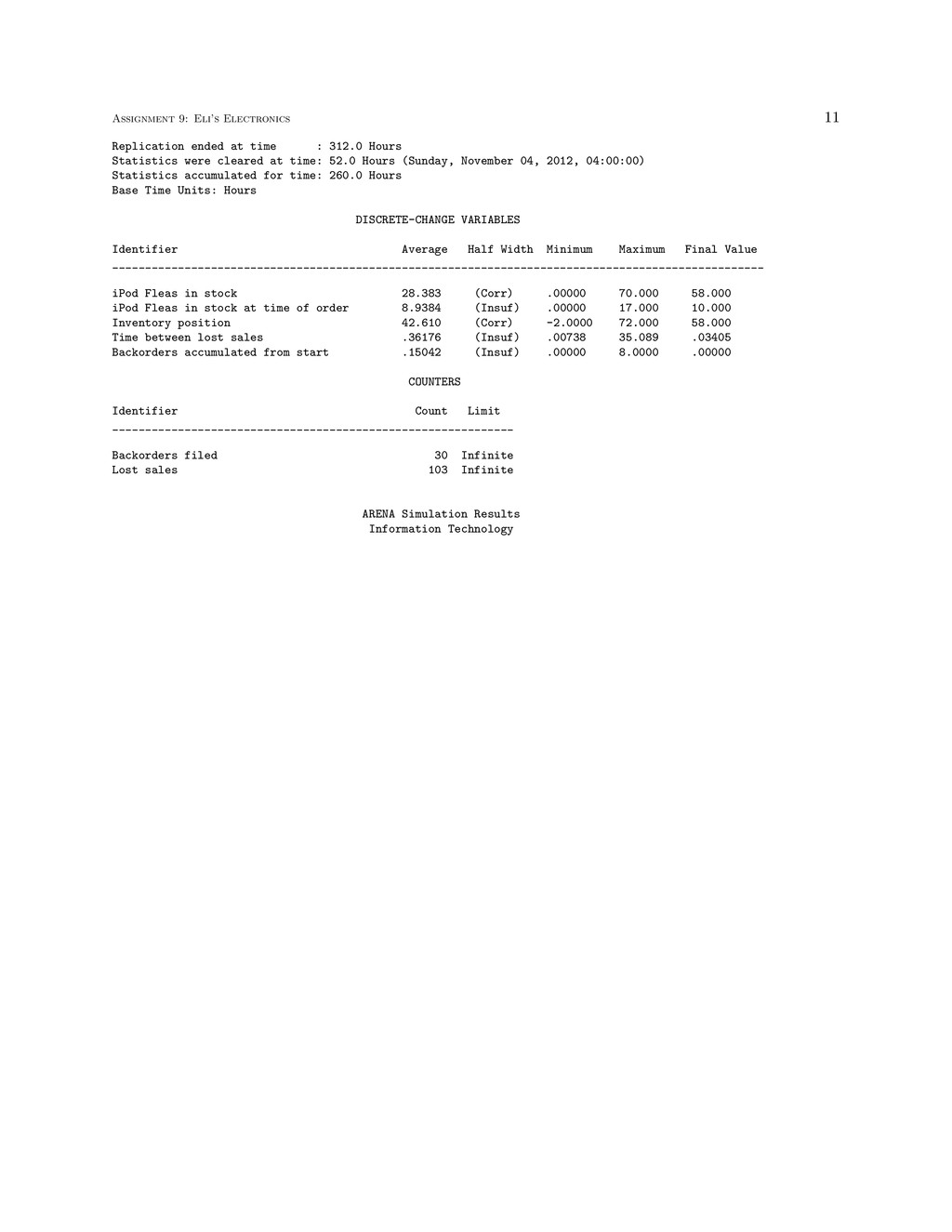
10. 10 M.Baker MakePlot("Inventory position and stock level for Eli’s Electronics", "Week number after warm-up period", "Number of iPod \’\’Fleas\’\’ in stock", 0, n, -8, stocklimit+17) EmpiricalADD( x= c(1:n), y=instock[1:n,5], ltystyle=2) EmpiricalADD( x= c(1:n), y=inventoryposition[1:n,5], ltystyle=3) legend(x=17.5, y=91, c("iPod \’\’Fleas\’\’ in stock at time t","iPod \’\’Flea\’\’ inventory position at time t"), lty=2:3) dev.off() safetystock.mean = mean(safetystock[2:31]) safetystock.sd = sd(safetystock[2:31]) safetystock.ci = qt(df=length(safetystock[2:31])-1, 1-alpha)*safetystock.sd/sqrt(length(safetystock[2:31])) safetystock.upper = safetystock.mean + safetystock.ci safetystock.lower = safetystock.mean - safetystock.ci postscript(file="hw9-safetystock.eps", width=10, height=7) MakePlot("95% Confidence interval for safety stock","Replication number","Safety stock level",0,31,0,18) points(safetystock.lower, pch=24, pty=3) points(safetystock.upper, pch=25, pty=3) points(safetystock.mean, lty=1, type="l") legend( x = 18, y=17, c("Upper confidence", "Sample mean", "Lower confidence"), pch=c(25,-1,24), lty=c(0,1,0)) dev.off() rm(lostsales.sum) lostsales.sum = rep(0,length(lostsales[,2:31])) k = 1 for ( i in lostsales[,2:31]){ lostsales.sum[k] = sum(i) k = k+1 } rm(backorders.sum) backorders.sum = rep(0,length(backorders[,2:31])) k = 1 for ( i in backorders[,2:31]){ backorders.sum[k] = sum(i) k = k+1 } postscript(file = "hw9-autocorrelation.eps", width = 10, height = 4) acf(c(backorders.sum, lostsales.sum), lag=80, main="Autocorrelation between time between lost sales and back orders", ylim=c(-1,1), xlab="Lag (sale number)") dev.off() for( i in c(1:length(backorders))){ print(c("You are watching replication",i)) acf(c(backorders[,i], lostsales[,i]), lag=500, main="Autocorrelation between lost sales and back orders", ylim=c(-1,1)) Sys.sleep(1) } C Output One replication of the SIMAN output is attached for the airline counter problem. The output file for the main problem: ARENA Simulation Results Information Technology Summary for Replication 1 of 30 Project: Elis Electronic Store Run execution date :11/ 2/2012 Analyst: Myles Baker Model revision date:11/ 2/2012
11. Assignment 9: Eli’s Electronics 11 Replication ended at time : 312.0 Hours Statistics were cleared at time: 52.0 Hours (Sunday, November 04, 2012, 04:00:00) Statistics accumulated for time: 260.0 Hours Base Time Units: Hours DISCRETE-CHANGE VARIABLES Identifier Average Half Width Minimum Maximum Final Value ___________________________________________________________________________________________________ iPod Fleas in stock 28.383 (Corr) .00000 70.000 58.000 iPod Fleas in stock at time of order 8.9384 (Insuf) .00000 17.000 10.000 Inventory position 42.610 (Corr) -2.0000 72.000 58.000 Time between lost sales .36176 (Insuf) .00738 35.089 .03405 Backorders accumulated from start .15042 (Insuf) .00000 8.0000 .00000 COUNTERS Identifier Count Limit _____________________________________________________________ Backorders filed 30 Infinite Lost sales 103 Infinite ARENA Simulation Results Information Technology