Learning, Prediction and Optimisation in RTB Display Advertising

CIKM16 Tutorial "Learning, Prediction and Optimisation in RTB Display Advertising" slide deck

Transcript

1. Learning, Prediction and Optimisation in RTB Display Advertising Weinan Zhang, Shanghai Jiao Tong University Jian Xu, TouchPal Inc. http://www.optimalrtb.com/cikm16/ October 24, 2016, Indianapolis, United States CIKM16 Tutorial
2. Speakers • Weinan Zhang – Assistant Professor at Shanghai Jiao Tong University – Ph.D. from University College London 2016 – Machine learning, data mining in computational advertising and recommender systems • Jian Xu – Principal Data Scientist at TouchPal, Mountain View – Previous Senior Data Scientist and Senior Research Engineer at Yahoo! US – Data mining, machine learning, and computational advertising
3. Tutorial Materials • Web site: http://www.optimalrtb.com/cikm16 • Supporting documents: – RTB monograph https://arxiv.org/abs/1610.03013 – RTB paper list: https://github.com/wnzhang/rtb-papers
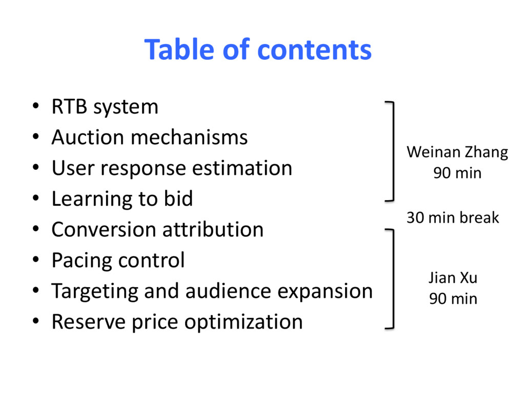
4. Table of contents • RTB system • Auction mechanisms • User response estimation • Learning to bid • Conversion attribution • Pacing control • Targeting and audience expansion • Reserve price optimization Weinan Zhang 90 min Jian Xu 90 min 30 min break
5. Table of contents • RTB system • Auction mechanisms • User response estimation • Learning to bid • Conversion attribution • Pacing control • Targeting and audience expansion • Reserve price optimization
6. Advertising • Make the best match between and with
7. - John Wanamaker (1838-1922) Father of modern advertising and a pioneer in marketing
8. Wasteful Traditional Advertising
9. Computational Advertising • Design algorithms to make the best match between the advertisers and Internet users with economic constraints
10. Search: iphone 6s case Sponsored Search
11. Sponsored Search • Advertiser sets a bid price for the keyword • User searches the keyword • Search engine hosts the auction to ranking the ads
12. Display Advertising http://www.nytimes.com/
13. Display Advertising • Advertiser targets a segment of users • Intermediary matches users and ads by user information
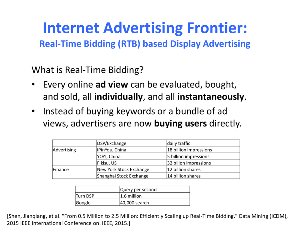
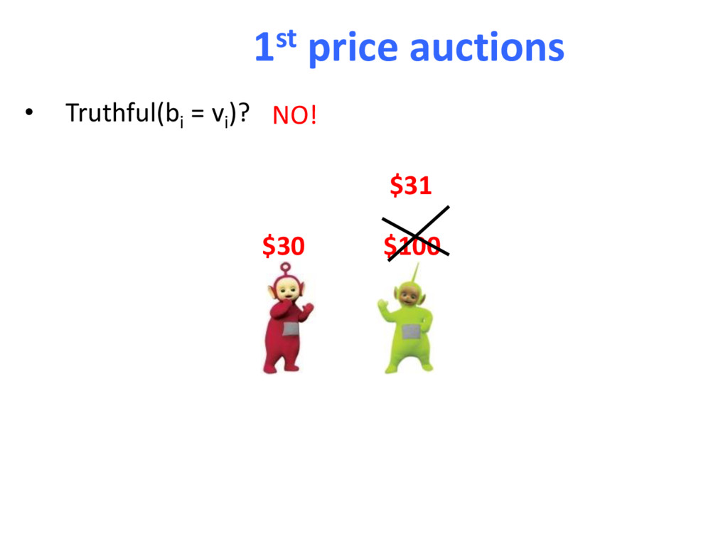
14. Internet Advertising Frontier: Real-Time Bidding (RTB) based Display Advertising What is Real-Time Bidding? • Every online ad view can be evaluated, bought, and sold, all individually, and all instantaneously. • Instead of buying keywords or a bundle of ad views, advertisers are now buying users directly. DSP/Exchange daily traffic Advertising iPinYou, China 18 billion impressions YOYI, China 5 billion impressions Fikisu, US 32 billon impressions Finance New York Stock Exchange 12 billion shares Shanghai Stock Exchange 14 billion shares Query per second Turn DSP 1.6 million Google 40,000 search [Shen, Jianqiang, et al. "From 0.5 Million to 2.5 Million: Efficiently Scaling up Real-Time Bidding." Data Mining (ICDM), 2015 IEEE International Conference on. IEEE, 2015.]
15. Suppose a student regularly reads articles on emarketer.com Content-related ads
16. He recently checked the London hotels (In fact, no login is required)
17. Relevant ads on facebook.com
18. Even on supervisor’s homepage! (User targeting dominates the context)
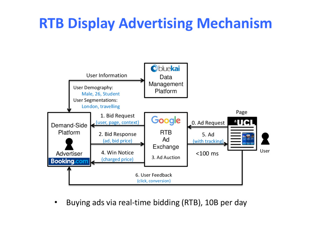
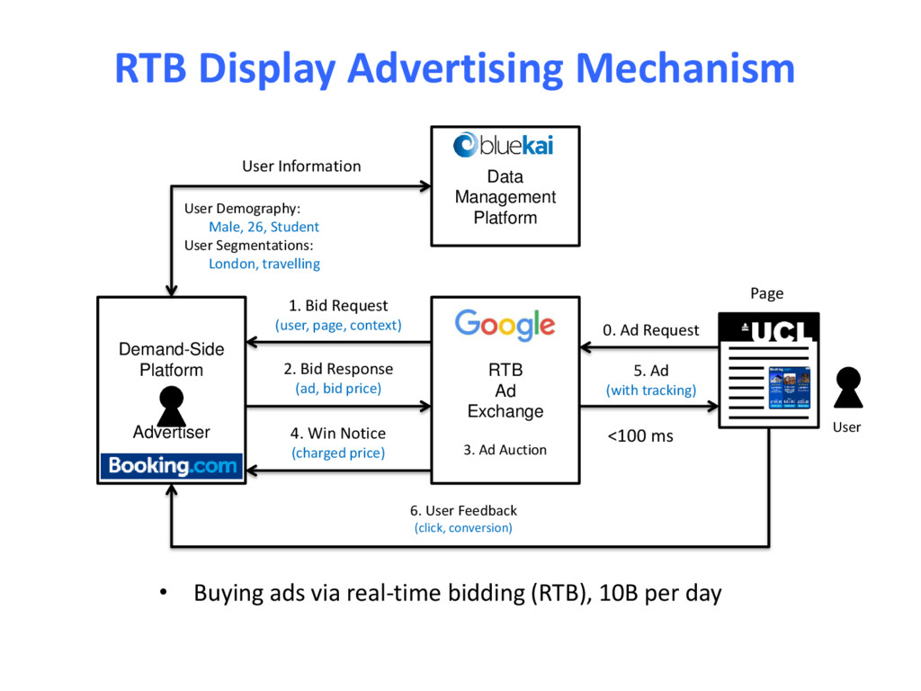
19. RTB Display Advertising Mechanism • Buying ads via real-time bidding (RTB), 10B per day RTB Ad Exchange Demand-Side Platform Advertiser Data Management Platform 0. Ad Request 1. Bid Request (user, page, context) 2. Bid Response (ad, bid price) 3. Ad Auction 4. Win Notice (charged price) 5. Ad (with tracking) 6. User Feedback (click, conversion) User Information User Demography: Male, 26, Student User Segmentations: London, travelling Page User <100 ms
20. Table of contents • RTB system • Auction mechanisms • User response estimation • Learning to bid • Conversion attribution • Pacing control • Targeting and audience expansion • Reserve price optimization
21. Auctions scheme v1 v2 v3 v4 b1 b2 b3 b4 private values bids winner payments $$$
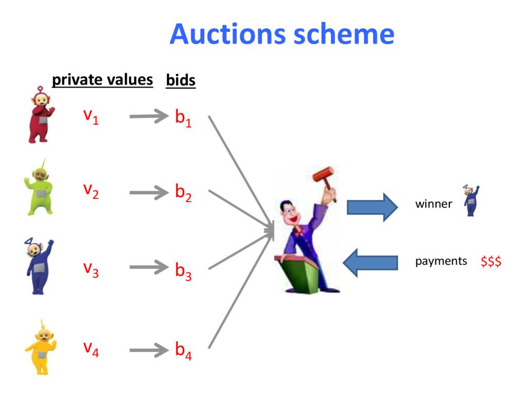
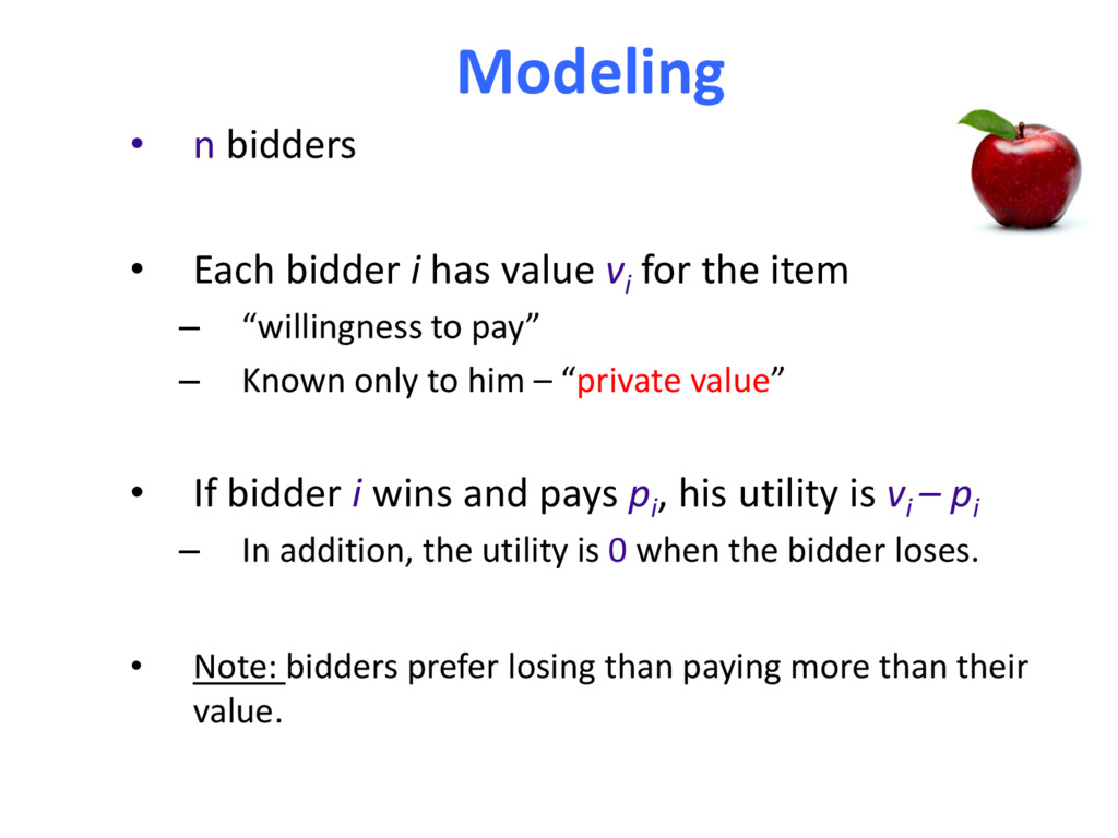
22. Modeling • n bidders • Each bidder i has value vi for the item – “willingness to pay” – Known only to him – “private value” • If bidder i wins and pays pi , his utility is vi – pi – In addition, the utility is 0 when the bidder loses. • Note: bidders prefer losing than paying more than their value.
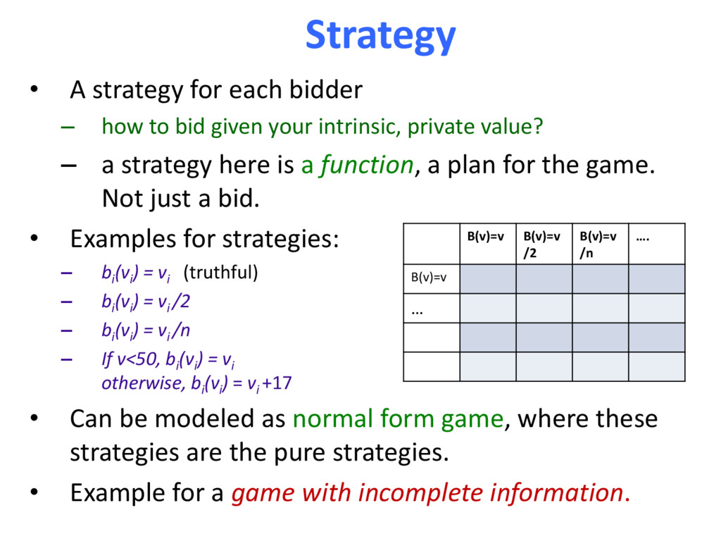
23. Strategy • A strategy for each bidder – how to bid given your intrinsic, private value? – a strategy here is a function, a plan for the game. Not just a bid. • Examples for strategies: – bi (vi ) = vi (truthful) – bi (vi ) = vi /2 – bi (vi ) = vi /n – If v<50, bi (vi ) = vi otherwise, bi (vi ) = vi +17 • Can be modeled as normal form game, where these strategies are the pure strategies. • Example for a game with incomplete information. B(v)=v B(v)=v /2 B(v)=v /n …. B(v)=v …
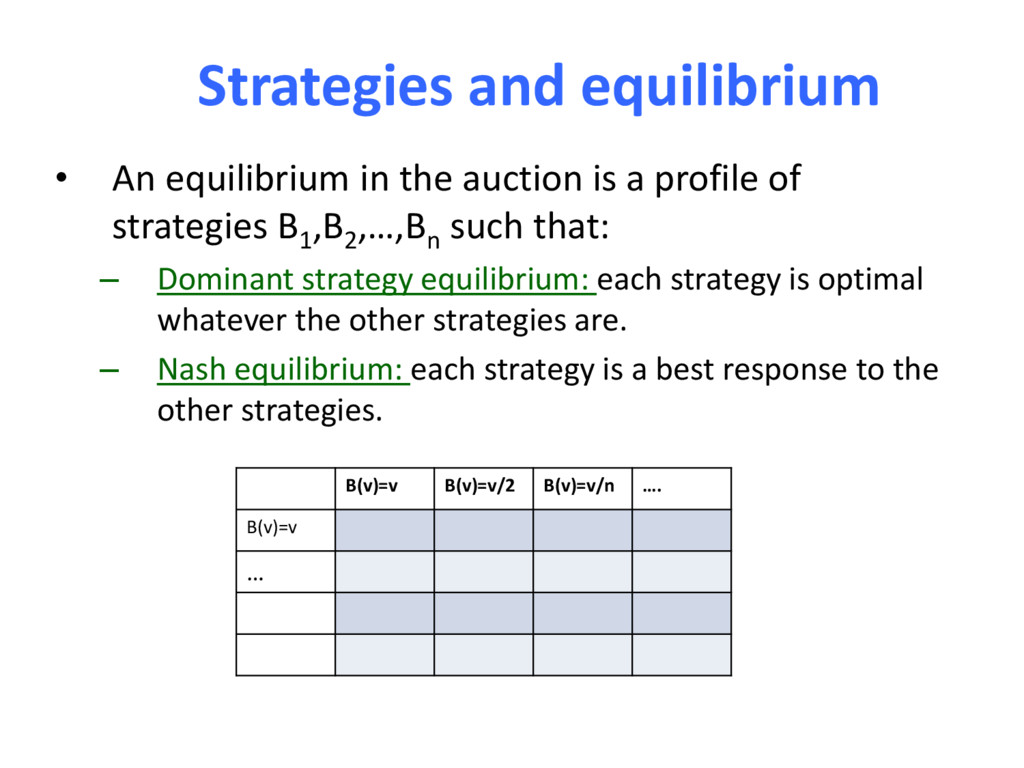
24. Strategies and equilibrium • An equilibrium in the auction is a profile of strategies B1 ,B2 ,…,Bn such that: – Dominant strategy equilibrium: each strategy is optimal whatever the other strategies are. – Nash equilibrium: each strategy is a best response to the other strategies. B(v)=v B(v)=v/2 B(v)=v/n …. B(v)=v …
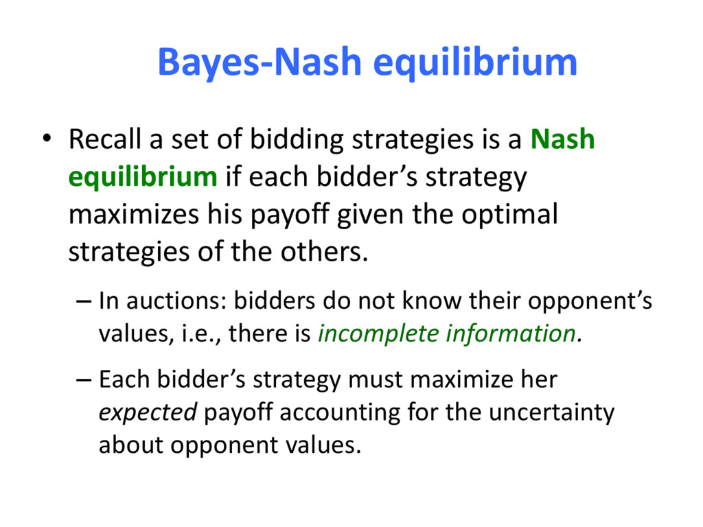
25. Bayes-Nash equilibrium • Recall a set of bidding strategies is a Nash equilibrium if each bidder’s strategy maximizes his payoff given the optimal strategies of the others. – In auctions: bidders do not know their opponent’s values, i.e., there is incomplete information. – Each bidder’s strategy must maximize her expected payoff accounting for the uncertainty about opponent values.
26. 1st price auctions • Truthful(bi = vi )? $30 $100 $31 NO!
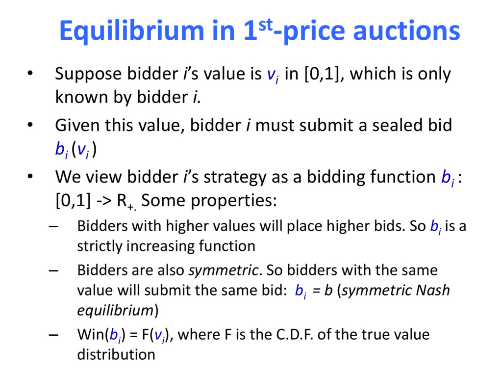
27. Equilibrium in 1st-price auctions • Suppose bidder i’s value is vi in [0,1], which is only known by bidder i. • Given this value, bidder i must submit a sealed bid bi (vi ) • We view bidder i’s strategy as a bidding function bi : [0,1] -> R+. Some properties: – Bidders with higher values will place higher bids. So bi is a strictly increasing function – Bidders are also symmetric. So bidders with the same value will submit the same bid: bi = b (symmetric Nash equilibrium) – Win(bi ) = F(vi ), where F is the C.D.F. of the true value distribution
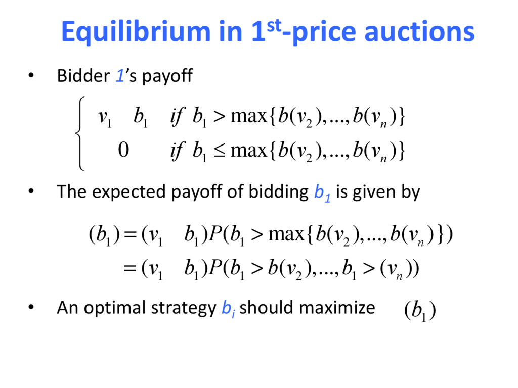
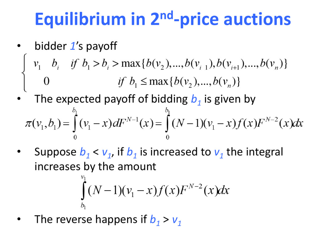
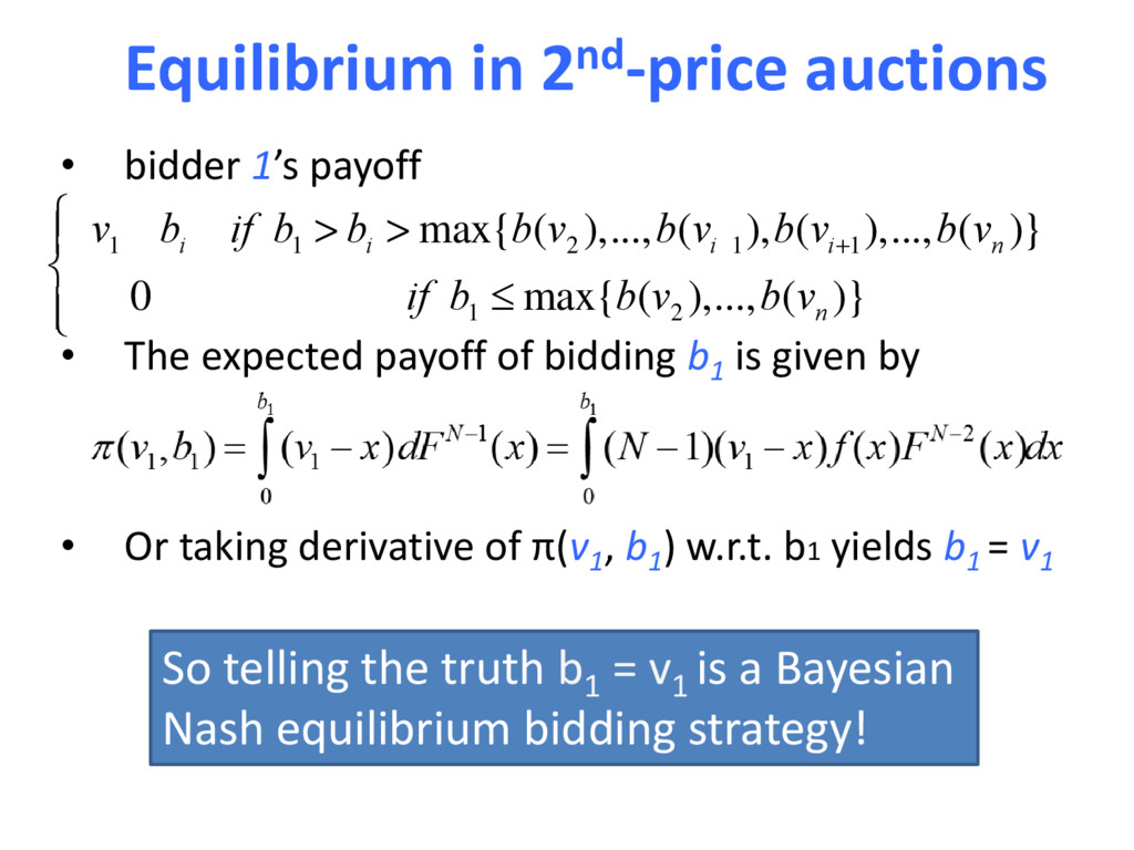
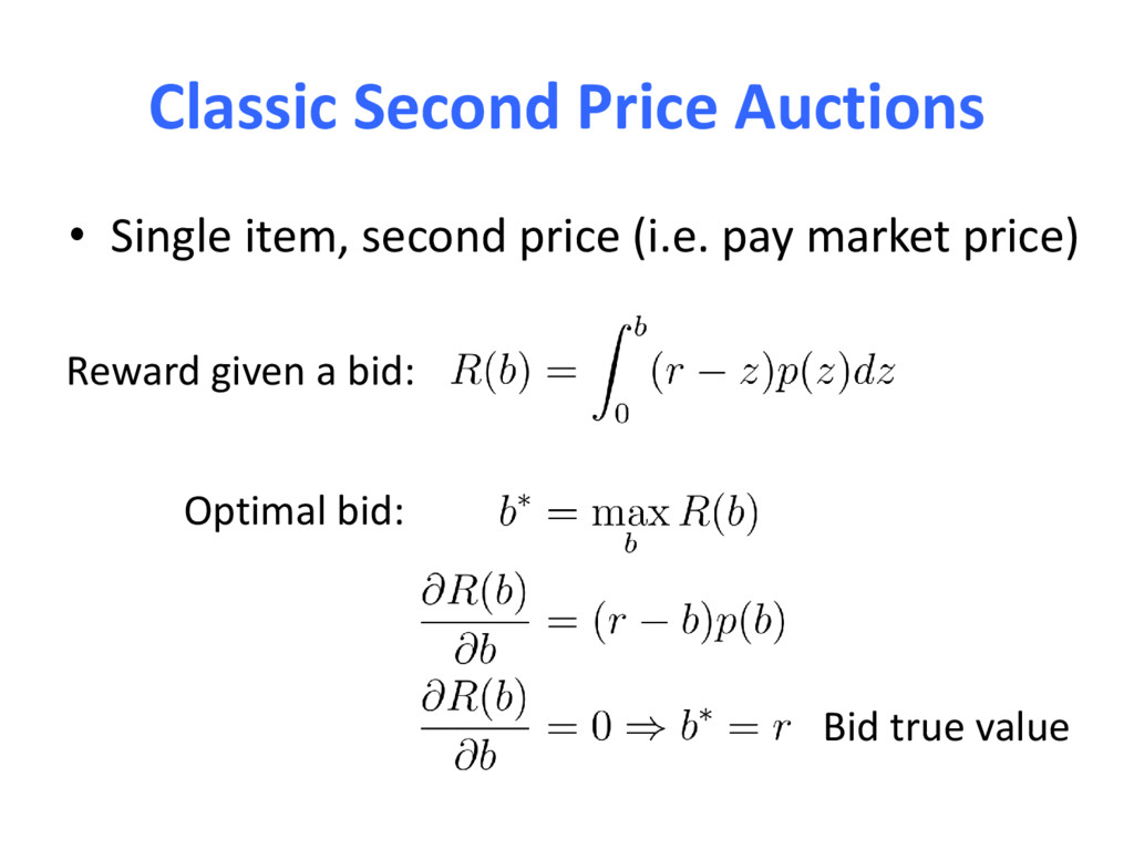
28. Equilibrium in 1st-price auctions • Bidder 1’s payoff • The expected payoff of bidding b1 is given by • An optimal strategy bi should maximize v 1 - b 1 if b 1 > max{b(v 2 ),...,b(v n )} 0 if b 1 £ max{b(v 2 ),...,b(v n )} ì í ï î ï p(b 1 ) = (v 1 - b 1 )P(b 1 > max{b(v 2 ),...,b(v n ) = (v 1 - b 1 )P(b 1 > b(v 2 ),...,b 1 > (v n )) p(b 1 ) })
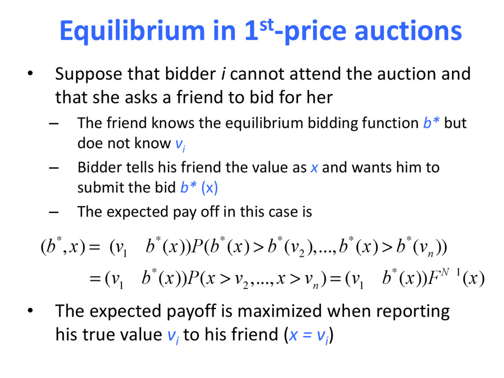
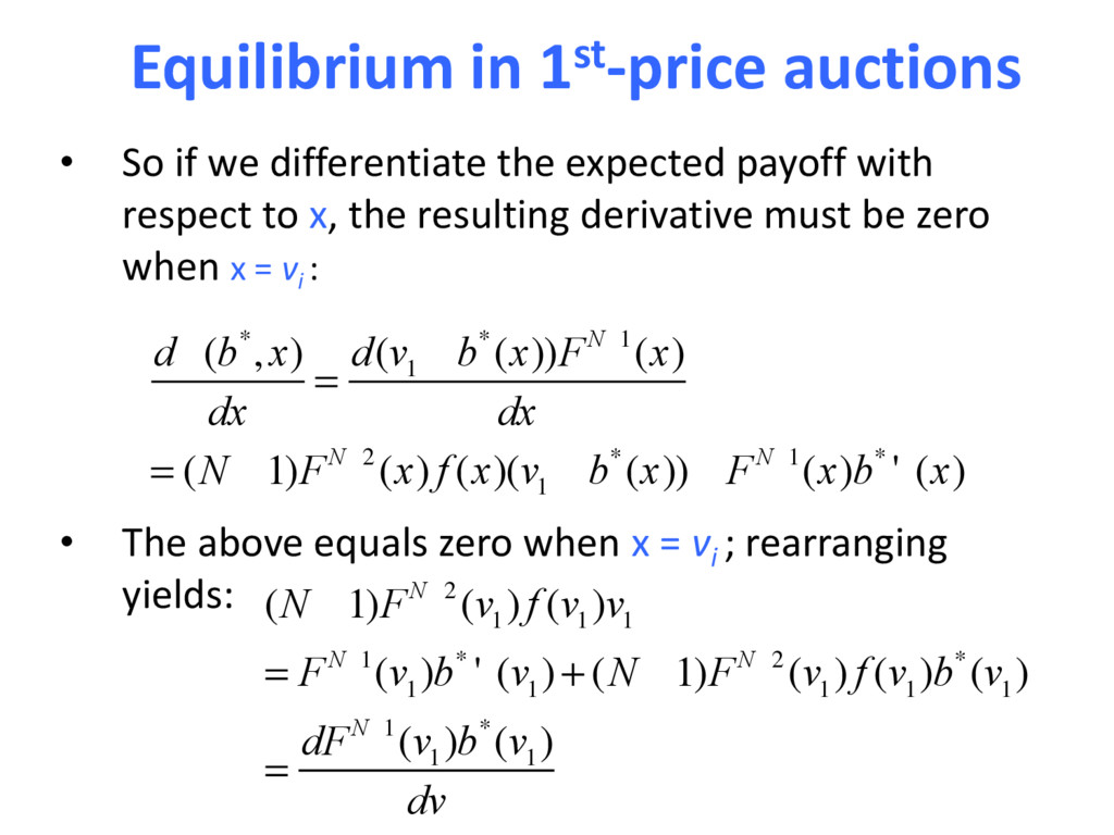
29. Equilibrium in 1st-price auctions • Suppose that bidder i cannot attend the auction and that she asks a friend to bid for her – The friend knows the equilibrium bidding function b* but doe not know vi – Bidder tells his friend the value as x and wants him to submit the bid b* (x) – The expected pay off in this case is • The expected payoff is maximized when reporting his true value vi to his friend (x = vi ) p(b*,x) = (v 1 - b*(x))P(b*(x) > b*(v 2 ),...,b*(x) > b*(v n )) = (v 1 - b*(x))P(x > v 2 ,...,x > v n ) = (v 1 - b*(x))FN-1(x)
30. Equilibrium in 1st-price auctions • So if we differentiate the expected payoff with respect to x, the resulting derivative must be zero when x = vi : • The above equals zero when x = vi ; rearranging yields: dp(b*,x) dx = d(v 1 - b*(x))FN-1(x) dx = (N -1)FN-2 (x) f (x)(v 1 - b*(x))- FN-1(x)b* ' (x) (N -1)FN-2 (v 1 ) f (v 1 )v 1 = FN-1(v 1 )b* ' (v 1 )+ (N -1)FN-2 (v 1 ) f (v 1 )b*(v 1 ) = dFN-1(v 1 )b*(v 1 ) dv
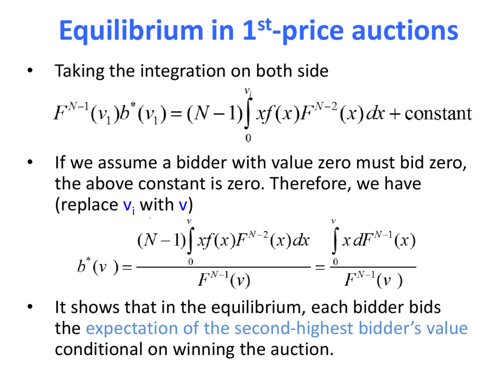
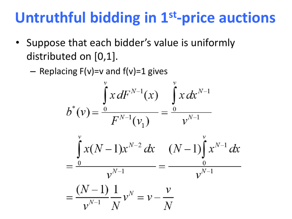
31. Equilibrium in 1st-price auctions • Taking the integration on both side • If we assume a bidder with value zero must bid zero, the above constant is zero. Therefore, we have (replace vi with v) • It shows that in the equilibrium, each bidder bids the expectation of the second-highest bidder’s value conditional on winning the auction.
32. Untruthful bidding in 1st-price auctions • Suppose that each bidder’s value is uniformly distributed on [0,1]. – Replacing F(v)=v and f(v)=1 gives
33. Equilibrium in 2nd-price auctions • bidder 1’s payoff • The expected payoff of bidding b1 is given by • Suppose b1 < v1 , if b1 is increased to v1 the integral increases by the amount • The reverse happens if b1 > v1 v 1 - b i if b 1 > b i > max{b(v 2 ),...,b(v i-1 ),b(v i+1 ),...,b(v n )} 0 if b 1 £ max{b(v 2 ),...,b(v n )} ì í ï î ï
34. Equilibrium in 2nd-price auctions • bidder 1’s payoff • The expected payoff of bidding b1 is given by • Or taking derivative of π(v1 , b1 ) w.r.t. b1 yields b1 = v1 v 1 - b i if b 1 > b i > max{b(v 2 ),...,b(v i-1 ),b(v i+1 ),...,b(v n )} 0 if b 1 £ max{b(v 2 ),...,b(v n )} ì í ï î ï So telling the truth b1 = v1 is a Bayesian Nash equilibrium bidding strategy!
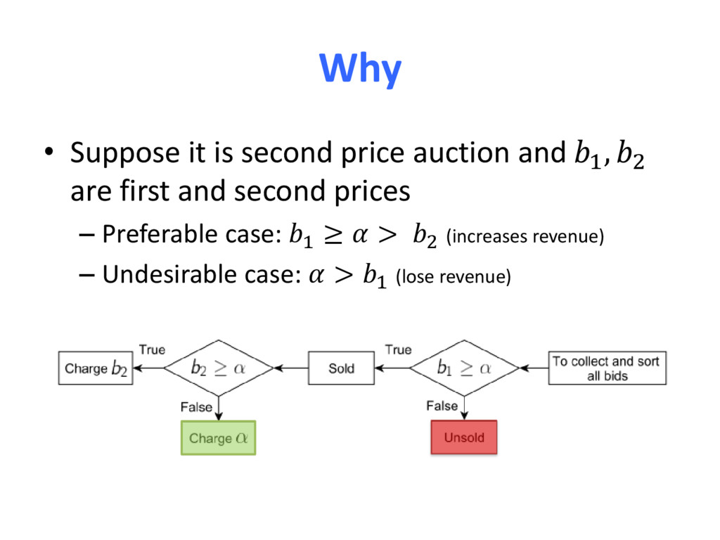
35. Reserve Prices and Entry Fees • Reserve Prices: the seller is assumed to have committed to not selling below the reserve – Reserve prices are assumed to be known to all bidders – The reserve prices = the minimum bids • Entry Fees: those bidders who enter have to pay the entry fee to the seller • They reduce bidders’ incentives to participate, but they might increase revenue as – 1) the seller collects extra revenues – 2) bidders might bid more aggressively
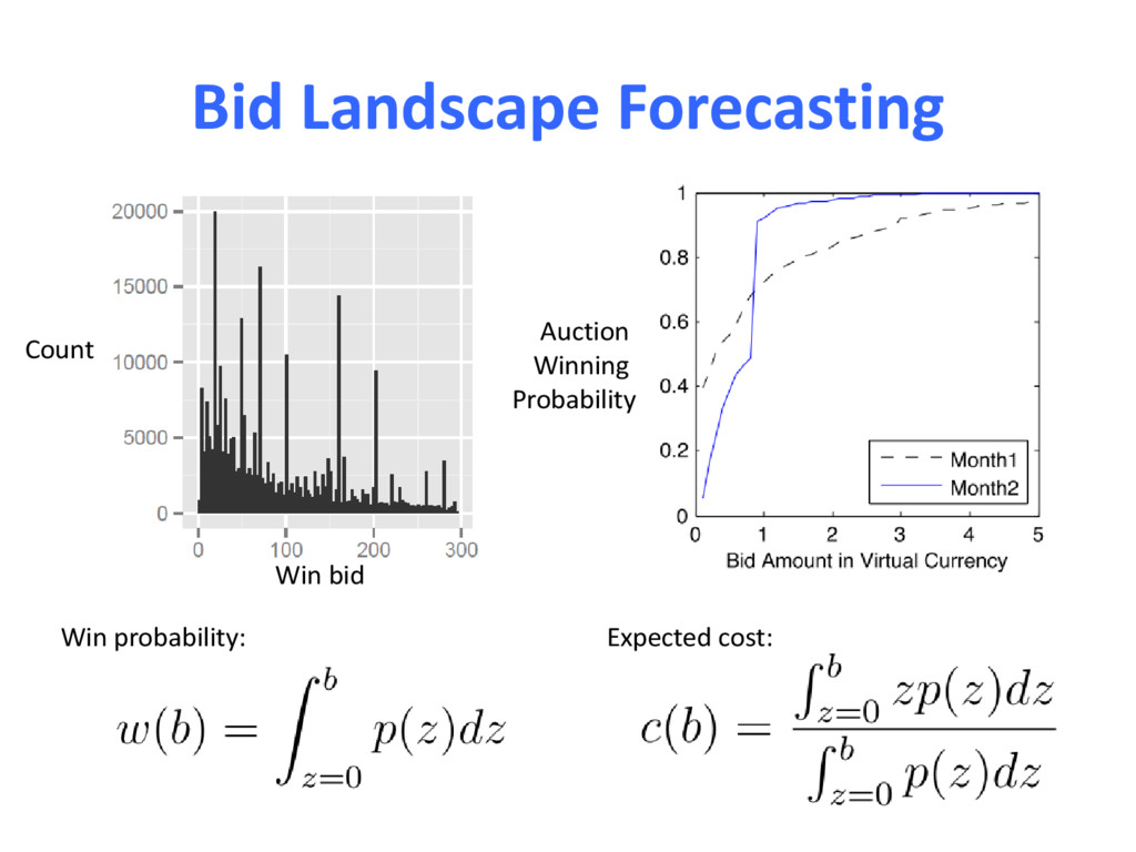
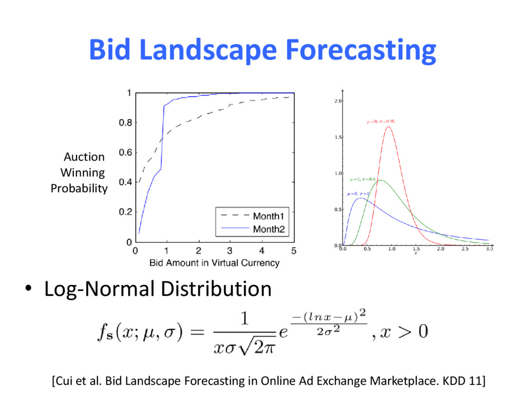
36. RTB Auctions • Second price auction with reserve price • From a bidder’s perspective, the market price z refers to the highest bid from competitors • Payoff: (vimpression – z) × P(win) • Value of impression depends on user response
37. Table of contents • RTB system • Auction mechanisms • User response estimation • Learning to bid • Conversion attribution • Pacing control • Targeting and audience expansion • Reserve price optimization
38. RTB Display Advertising Mechanism • Buying ads via real-time bidding (RTB), 10B per day RTB Ad Exchange Demand-Side Platform Advertiser Data Management Platform 0. Ad Request 1. Bid Request (user, page, context) 2. Bid Response (ad, bid price) 3. Ad Auction 4. Win Notice (charged price) 5. Ad (with tracking) 6. User Feedback (click, conversion) User Information User Demography: Male, 26, Student User Segmentations: London, travelling Page User <100 ms
39. Predict how likely the user is going to click the displayed ad.
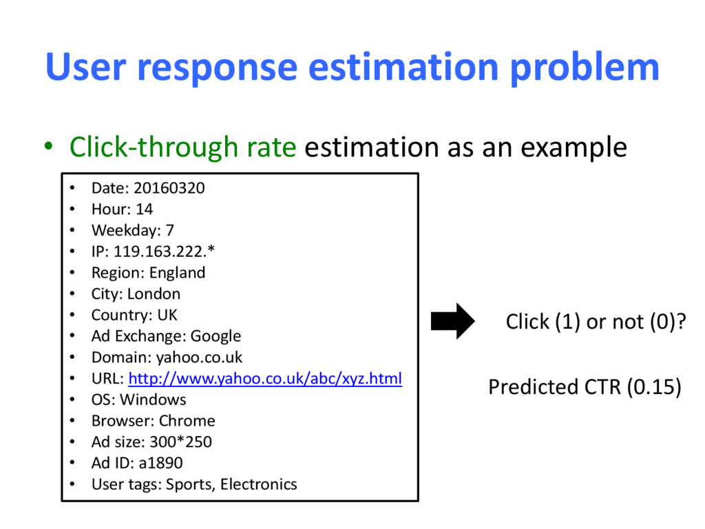
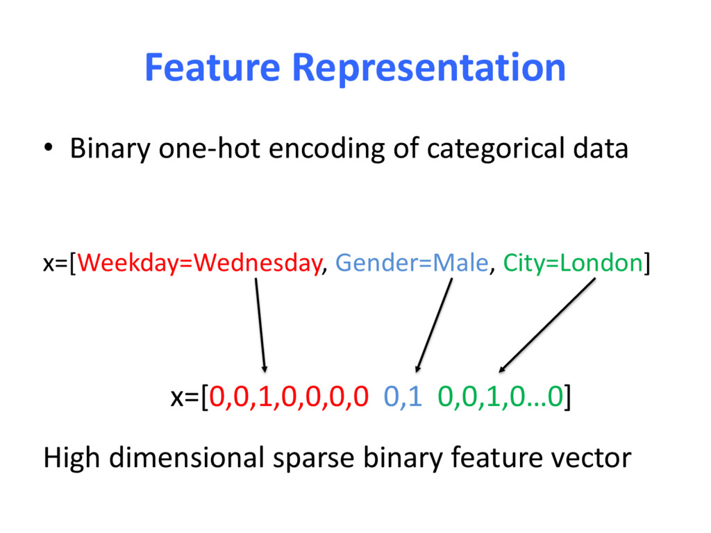
40. User response estimation problem • Click-through rate estimation as an example • Date: 20160320 • Hour: 14 • Weekday: 7 • IP: 119.163.222.* • Region: England • City: London • Country: UK • Ad Exchange: Google • Domain: yahoo.co.uk • URL: http://www.yahoo.co.uk/abc/xyz.html • OS: Windows • Browser: Chrome • Ad size: 300*250 • Ad ID: a1890 • User tags: Sports, Electronics Click (1) or not (0)? Predicted CTR (0.15)
41. Feature Representation • Binary one-hot encoding of categorical data x=[Weekday=Wednesday, Gender=Male, City=London] x=[0,0,1,0,0,0,0 0,1 0,0,1,0…0] High dimensional sparse binary feature vector
42. Linear Models • Logistic Regression – With SGD learning – Sparse solution • Online Bayesian Probit Regression
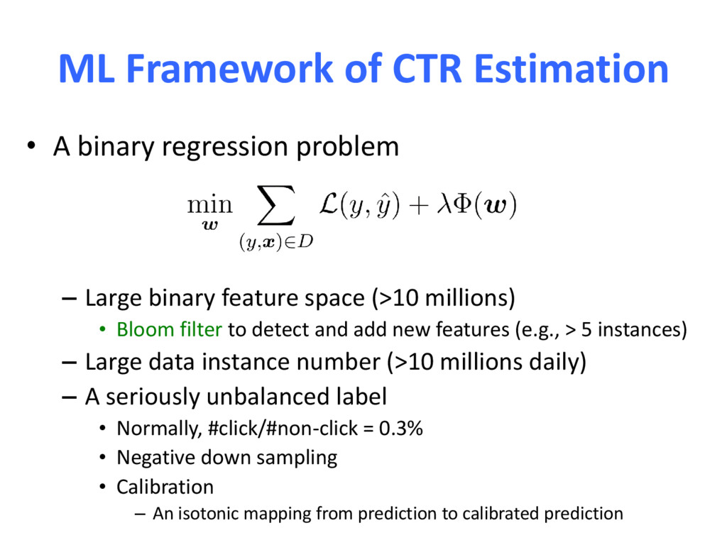
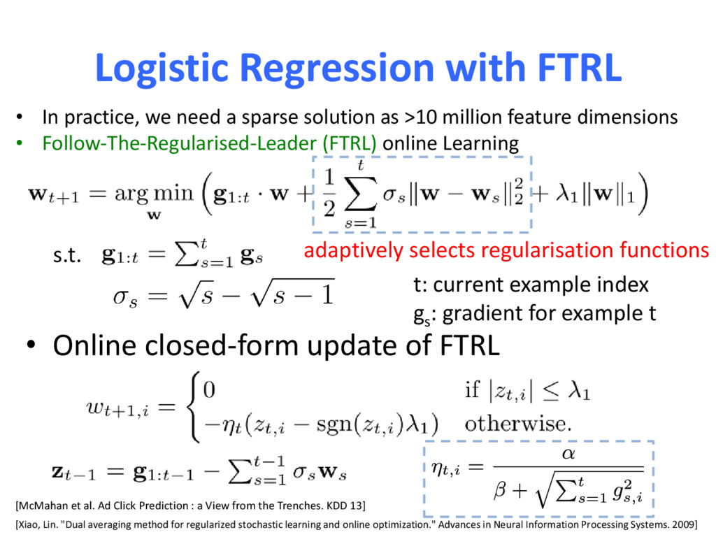
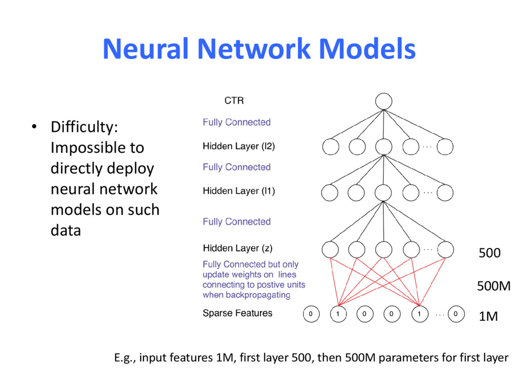
43. ML Framework of CTR Estimation • A binary regression problem – Large binary feature space (>10 millions) • Bloom filter to detect and add new features (e.g., > 5 instances) – Large data instance number (>10 millions daily) – A seriously unbalanced label • Normally, #click/#non-click = 0.3% • Negative down sampling • Calibration – An isotonic mapping from prediction to calibrated prediction
44. Logistic Regression • Prediction • Cross Entropy Loss • Stochastic Gradient Descent Learning [Lee et al. Estimating Conversion Rate in Display Advertising from Past Performance Data. KDD 12]
45. Logistic Regression with SGD • Pros – Standardised, easily understood and implemented – Easy to be parallelised • Cons – Learning rate η initialisation – Uniform learning rate against different binary features
46. Logistic Regression with FTRL • In practice, we need a sparse solution as >10 million feature dimensions • Follow-The-Regularised-Leader (FTRL) online Learning [McMahan et al. Ad Click Prediction : a View from the Trenches. KDD 13] s.t. • Online closed-form update of FTRL t: current example index gs : gradient for example t adaptively selects regularisation functions [Xiao, Lin. "Dual averaging method for regularized stochastic learning and online optimization." Advances in Neural Information Processing Systems. 2009]
47. Online Bayesian Probit Regression to approximate message passing. In order full factorial structure of the likelihood, wo latent variables , and consider the density function which (5) n can be understood in terms of the ative process, which is also reflected in in Figure 1. Sample weights from the Gaussian alculate the score for x as the inner , such that . dd zero-mean Gaussian noise to obtain h that . etermine by a threshold on the noisy ro, such that . skills in TrueSkill after a hypothetical m team with known skill of zero. Given the Figure 1 together with Table 1 in the a update equations can be derived. 3.3.1. UPDATE EQUATIONS FOR ONLINE The update equations represent a mappin posterior parameter values based o pairs ̃ ̃ . In terms of calculation can viewed as following the m schedule towards the weights . We d variance for a given input as The update for the posterior parameters is ̃ ( ̃ * (
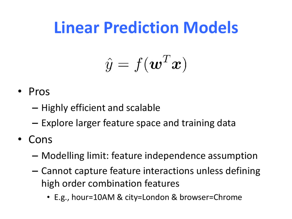
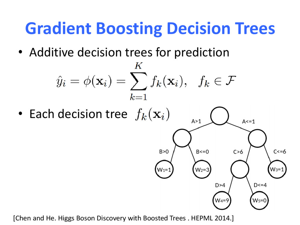
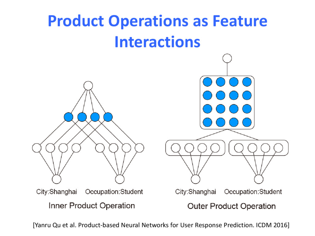
48. Linear Prediction Models • Pros – Highly efficient and scalable – Explore larger feature space and training data • Cons – Modelling limit: feature independence assumption – Cannot capture feature interactions unless defining high order combination features • E.g., hour=10AM & city=London & browser=Chrome
49. Non-linear Models • Factorisation Machines • Gradient Boosting Decision Trees • Combined Models • Deep Neural Networks
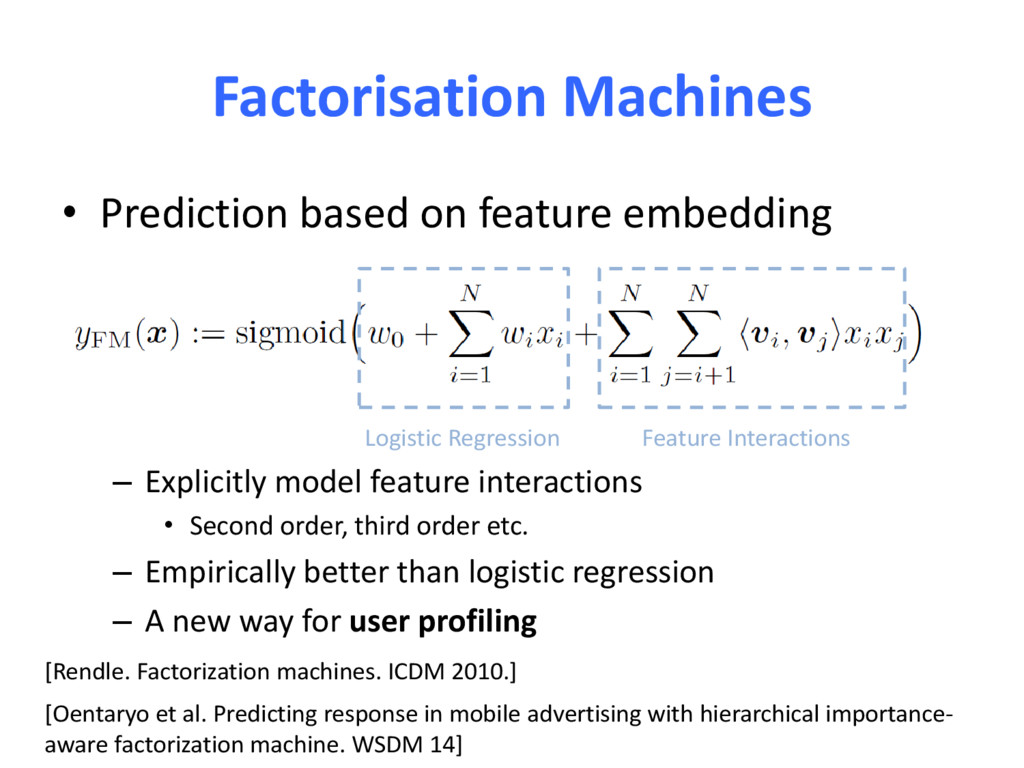
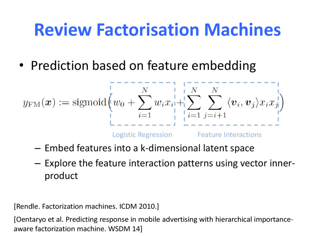
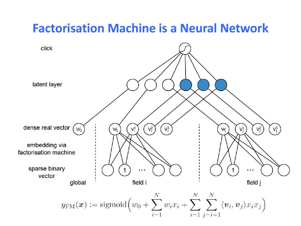
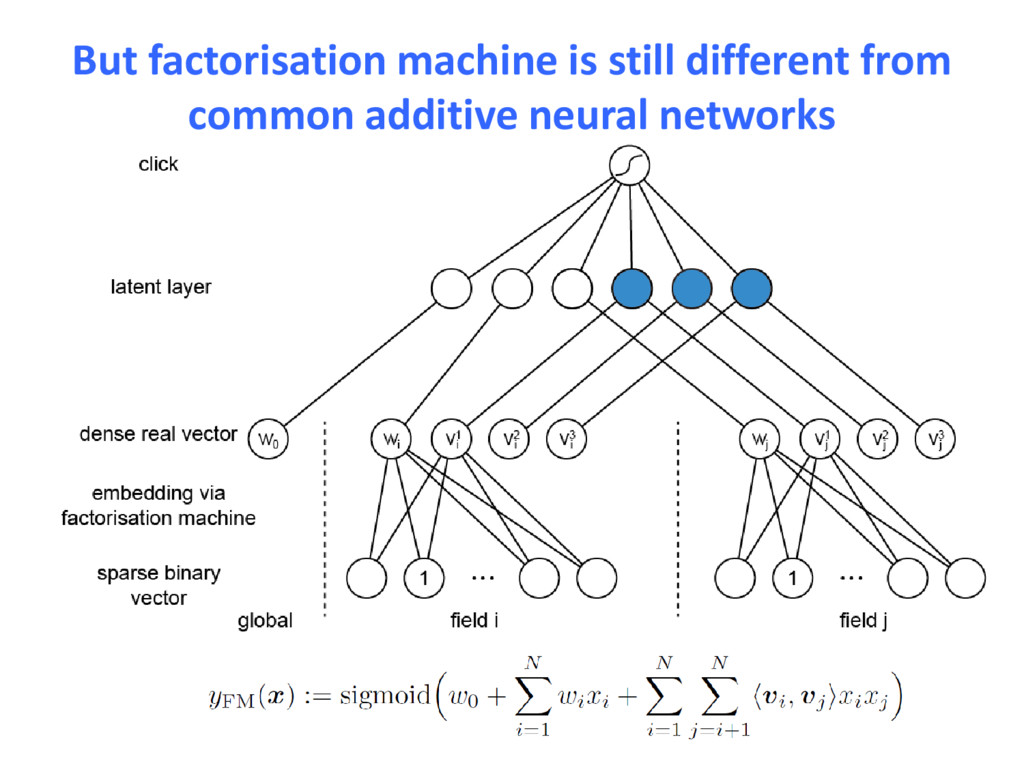
50. Factorisation Machines • Prediction based on feature embedding – Explicitly model feature interactions • Second order, third order etc. – Empirically better than logistic regression – A new way for user profiling [Oentaryo et al. Predicting response in mobile advertising with hierarchical importance- aware factorization machine. WSDM 14] [Rendle. Factorization machines. ICDM 2010.] Logistic Regression Feature Interactions
51. Factorisation Machines • Prediction based on feature embedding [Oentaryo et al. Predicting response in mobile advertising with hierarchical importance- aware factorization machine. WSDM 14] [Rendle. Factorization machines. ICDM 2010.] Logistic Regression Feature Interactions For x=[Weekday=Friday, Gender=Male, City=Shanghai]
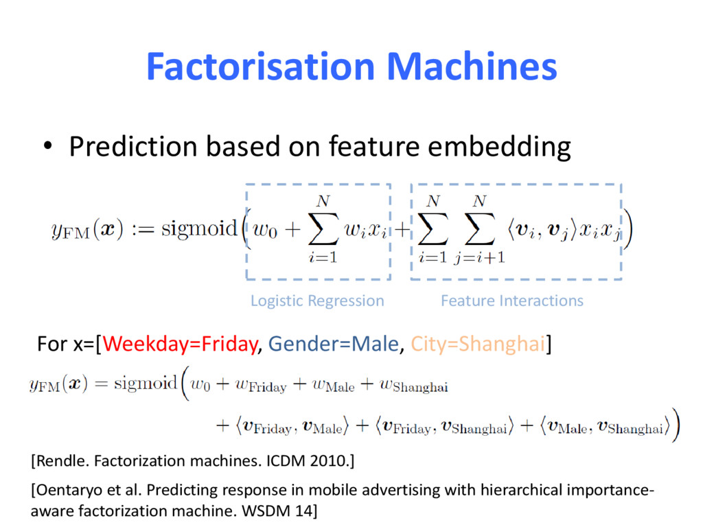
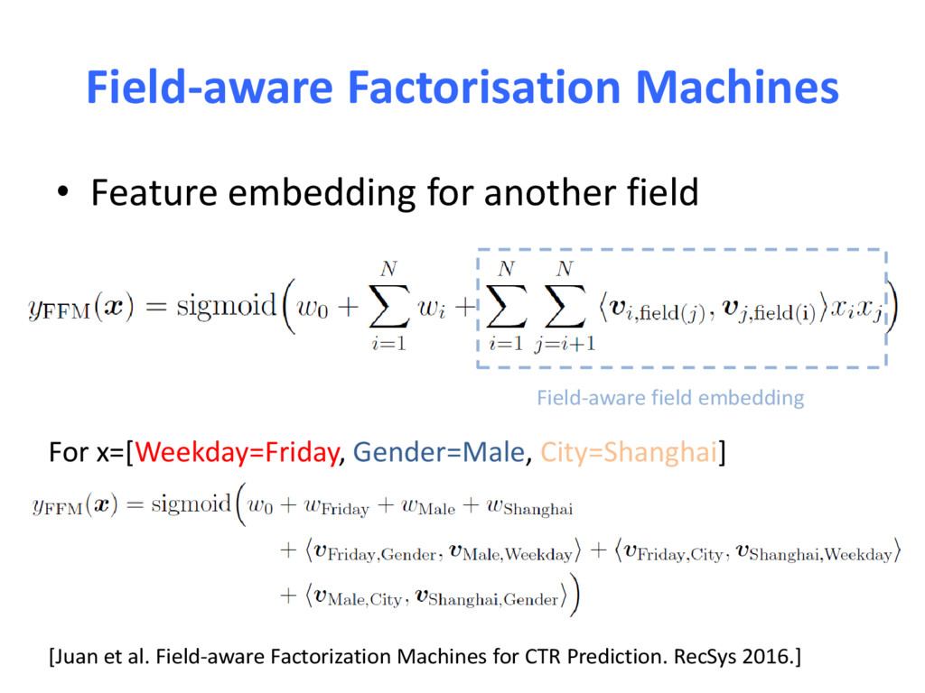
52. • Feature embedding for another field Field-aware Factorisation Machines [Juan et al. Field-aware Factorization Machines for CTR Prediction. RecSys 2016.] Field-aware field embedding For x=[Weekday=Friday, Gender=Male, City=Shanghai]
53. Gradient Boosting Decision Trees • Additive decision trees for prediction • Each decision tree [Chen and He. Higgs Boson Discovery with Boosted Trees . HEPML 2014.]
54. Gradient Boosting Decision Trees • Learning [Chen and He. Higgs Boson Discovery with Boosted Trees . HEPML 2014.] [Tianqi Chen. https://homes.cs.washington.edu/~tqchen/pdf/BoostedTree.pdf]
55. Combined Models: GBDT + LR [He et al. Practical Lessons from Predicting Clicks on Ads at Facebook . ADKDD 2014.]
56. Combined Models: GBDT + FM [http://www.csie.ntu.edu.tw/~r01922136/kaggle-2014-criteo.pdf]
57. Neural Network Models • Difficulty: Impossible to directly deploy neural network models on such data 1M 500 500M E.g., input features 1M, first layer 500, then 500M parameters for first layer
58. Review Factorisation Machines • Prediction based on feature embedding – Embed features into a k-dimensional latent space – Explore the feature interaction patterns using vector inner- product [Oentaryo et al. Predicting response in mobile advertising with hierarchical importance- aware factorization machine. WSDM 14] [Rendle. Factorization machines. ICDM 2010.] Logistic Regression Feature Interactions
59. Factorisation Machine is a Neural Network
60. [Zhang et al. Deep Learning over Multi-field Categorical Data – A Case Study on User Response Prediction. ECIR 16] [Factorisation Machine Initialised] Factorisation-machine supported Neural Networks (FNN)
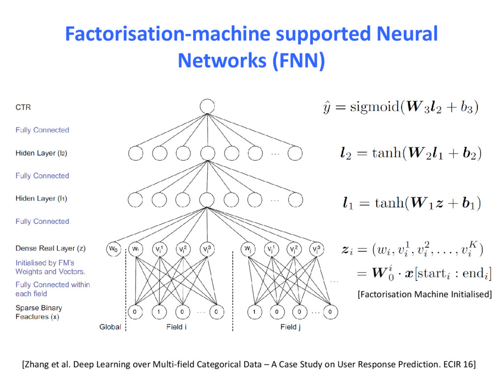
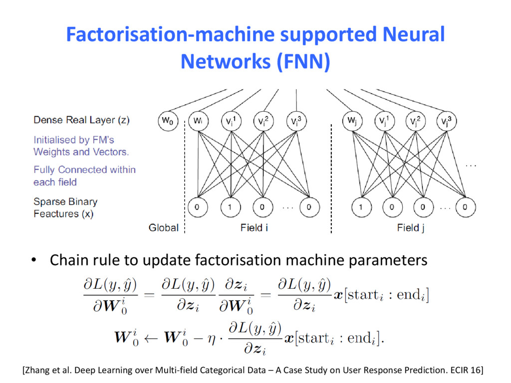
61. [Zhang et al. Deep Learning over Multi-field Categorical Data – A Case Study on User Response Prediction. ECIR 16] Factorisation-machine supported Neural Networks (FNN) • Chain rule to update factorisation machine parameters
62. But factorisation machine is still different from common additive neural networks
63. Product Operations as Feature Interactions [Yanru Qu et al. Product-based Neural Networks for User Response Prediction. ICDM 2016]
64. Product-based Neural Networks (PNN) Inner Product Or Outer Product [Yanru Qu et al. Product-based Neural Networks for User Response Prediction. ICDM 2016]
65. Convolutional Click Prediction Model (CCPM) • CNN to (partially) select good feature combinations [Qiang Liu et al. A convolutional click prediction model. CIKM 2015]
66. Overall Performance
67. Training with Instance Bias [Zhang et al. Bid-aware Gradient Descent for Unbiased Learning with Censored Data in Display Advertising. KDD 2016.]
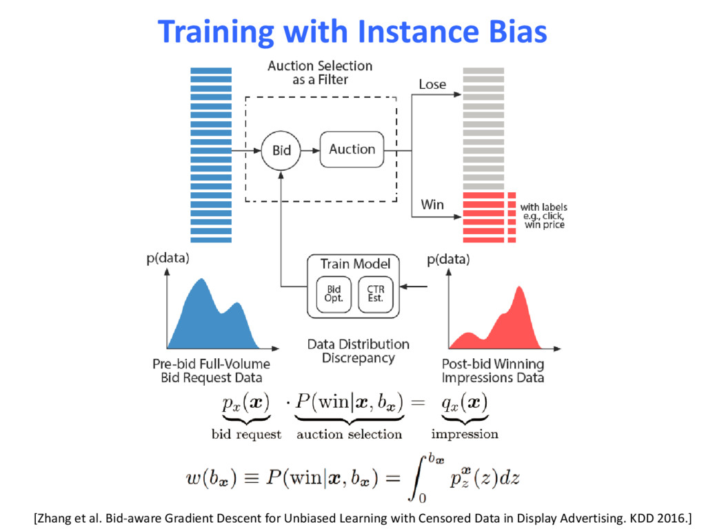
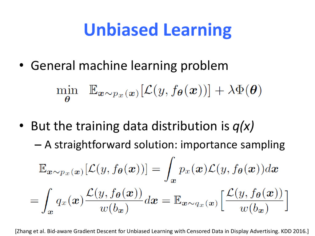
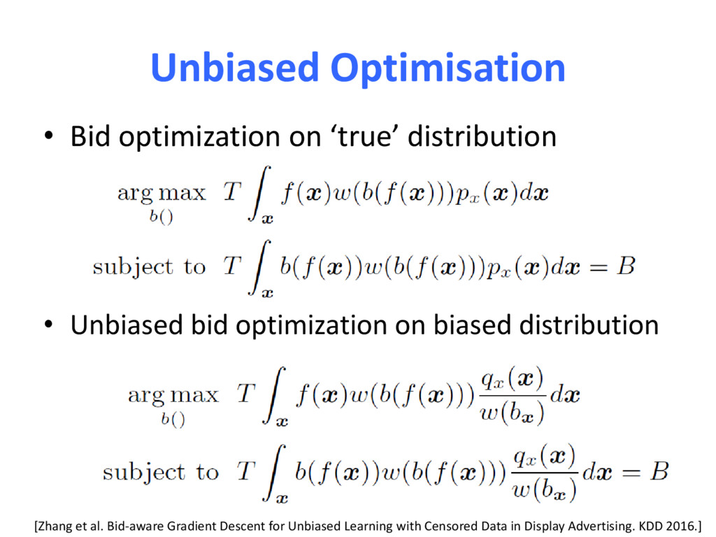
68. Unbiased Learning • General machine learning problem • But the training data distribution is q(x) – A straightforward solution: importance sampling [Zhang et al. Bid-aware Gradient Descent for Unbiased Learning with Censored Data in Display Advertising. KDD 2016.]
69. Unbiased CTR Estimator Learning [Zhang et al. Bid-aware Gradient Descent for Unbiased Learning with Censored Data in Display Advertising. KDD 2016.]
70. Table of contents • RTB system • Auction mechanisms • User response estimation • Learning to bid • Conversion attribution • Pacing control • Targeting and audience expansion • Reserve price optimization
71. RTB Display Advertising Mechanism • Buying ads via real-time bidding (RTB), 10B per day RTB Ad Exchange Demand-Side Platform Advertiser Data Management Platform 0. Ad Request 1. Bid Request (user, page, context) 2. Bid Response (ad, bid price) 3. Ad Auction 4. Win Notice (charged price) 5. Ad (with tracking) 6. User Feedback (click, conversion) User Information User Demography: Male, 26, Student User Segmentations: London, travelling Page User <100 ms
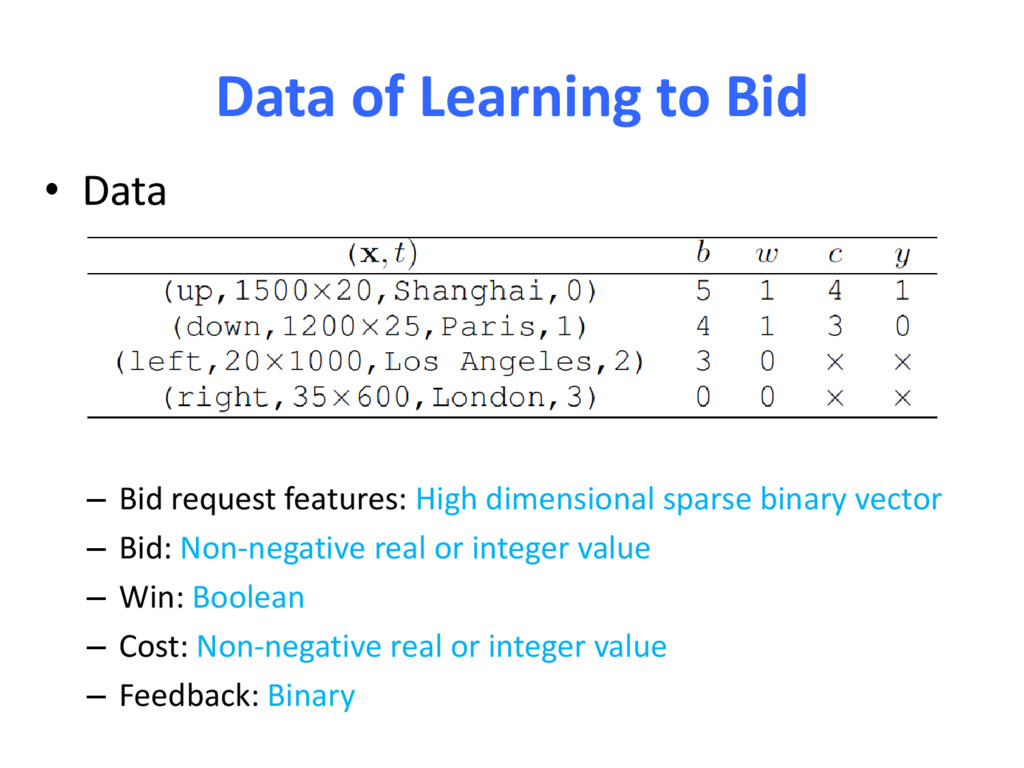
72. Data of Learning to Bid – Bid request features: High dimensional sparse binary vector – Bid: Non-negative real or integer value – Win: Boolean – Cost: Non-negative real or integer value – Feedback: Binary • Data
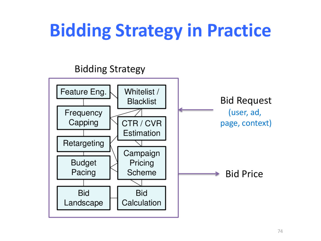
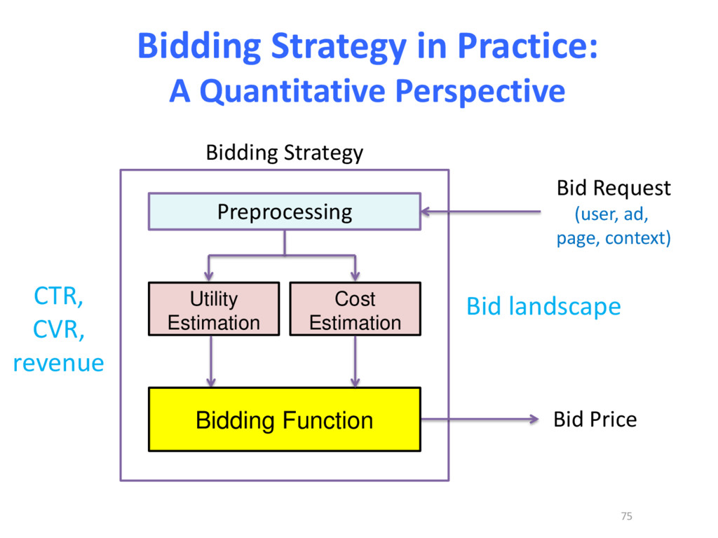
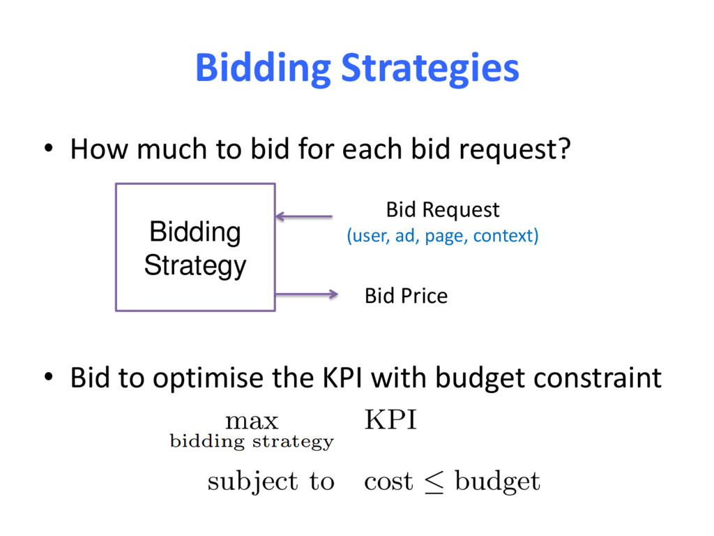
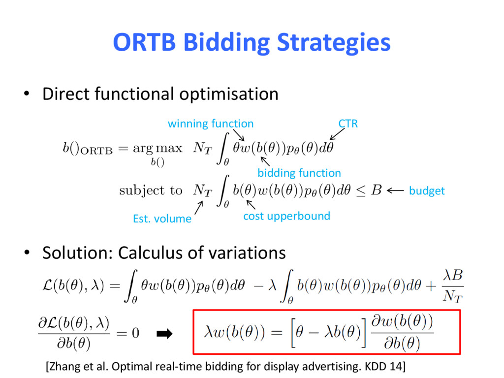
73. Problem Definition of Learning to Bid • How much to bid for each bid request? – Find an optimal bidding function b(x) • Bid to optimise the KPI with budget constraint Bid Request (user, ad, page, context) Bid Price Bidding Strategy
74. Bidding Strategy in Practice Bid Request (user, ad, page, context) Bid Price Bidding Strategy Feature Eng. Whitelist / Blacklist Retargeting Budget Pacing Bid Landscape Bid Calculation Frequency Capping CTR / CVR Estimation Campaign Pricing Scheme 74
75. Bidding Strategy in Practice: A Quantitative Perspective Bid Request (user, ad, page, context) Bid Price Bidding Strategy Utility Estimation Cost Estimation Preprocessing Bidding Function CTR, CVR, revenue Bid landscape 75
76. Bid Landscape Forecasting Auction Winning Probability Win probability: Expected cost: Count Win bid
77. Bid Landscape Forecasting • Log-Normal Distribution Auction Winning Probability [Cui et al. Bid Landscape Forecasting in Online Ad Exchange Marketplace. KDD 11]
78. Bid Landscape Forecasting • Price Prediction via Linear Regression – Modelling censored data in lost bid requests [Wu et al. Predicting Winning Price in Real Time Bidding with Censored Data. KDD 15]
79. Survival Tree Models [Yuchen Wang et al. Functional Bid Landscape Forecasting for Display Advertising. ECMLPKDD 2016 ] Node split Based on Clustering categories
80. Bidding Strategies • How much to bid for each bid request? • Bid to optimise the KPI with budget constraint Bid Request (user, ad, page, context) Bid Price Bidding Strategy
81. Classic Second Price Auctions • Single item, second price (i.e. pay market price) Reward given a bid: Optimal bid: Bid true value
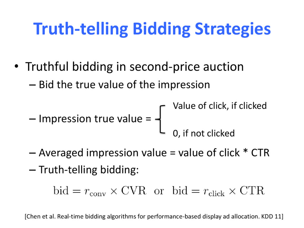
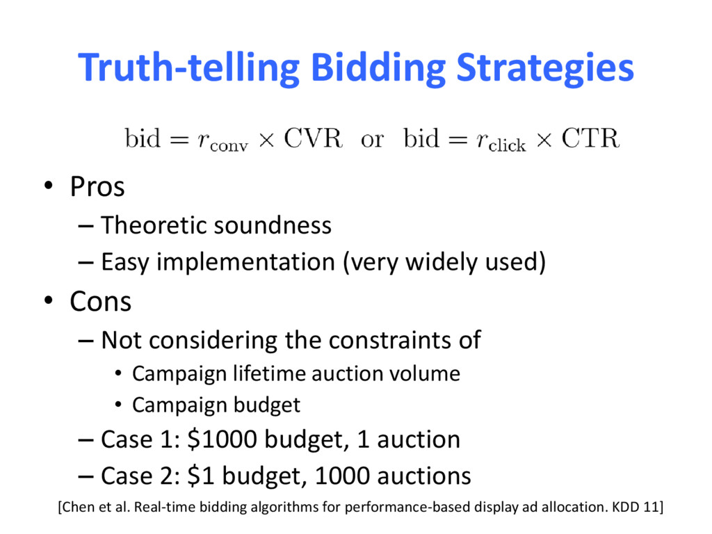
82. Truth-telling Bidding Strategies • Truthful bidding in second-price auction – Bid the true value of the impression – Impression true value = – Averaged impression value = value of click * CTR – Truth-telling bidding: [Chen et al. Real-time bidding algorithms for performance-based display ad allocation. KDD 11] Value of click, if clicked 0, if not clicked
83. Truth-telling Bidding Strategies • Pros – Theoretic soundness – Easy implementation (very widely used) • Cons – Not considering the constraints of • Campaign lifetime auction volume • Campaign budget – Case 1: $1000 budget, 1 auction – Case 2: $1 budget, 1000 auctions [Chen et al. Real-time bidding algorithms for performance-based display ad allocation. KDD 11]
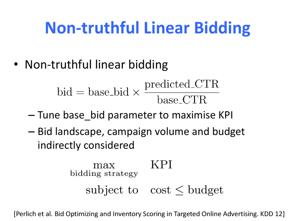
84. Non-truthful Linear Bidding • Non-truthful linear bidding – Tune base_bid parameter to maximise KPI – Bid landscape, campaign volume and budget indirectly considered [Perlich et al. Bid Optimizing and Inventory Scoring in Targeted Online Advertising. KDD 12]
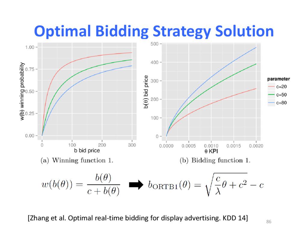
85. ORTB Bidding Strategies • Direct functional optimisation CTR winning function bidding function budget Est. volume cost upperbound [Zhang et al. Optimal real-time bidding for display advertising. KDD 14] • Solution: Calculus of variations
86. Optimal Bidding Strategy Solution 86 [Zhang et al. Optimal real-time bidding for display advertising. KDD 14]
87. Unbiased Optimisation • Bid optimization on ‘true’ distribution • Unbiased bid optimization on biased distribution [Zhang et al. Bid-aware Gradient Descent for Unbiased Learning with Censored Data in Display Advertising. KDD 2016.]
88. Unbiased Bid Optimisation A/B Testing on Yahoo! DSP. [Zhang et al. Bid-aware Gradient Descent for Unbiased Learning with Censored Data in Display Advertising. KDD 2016.]
89. That’s the first half of the tutorial! Questions?
90. Part 2 Speaker: Jian Xu, TouchPal Inc. (jian.xu AT cootek.cn) CIKM16 Tutorial
91. Part 2 Speaker: Jian Xu, TouchPal Inc. usjobs@cootek.cn
92. Table of contents • RTB system • Auction mechanisms • User response estimation • Learning to bid • Conversion attribution • Pacing control • Targeting and audience expansion • Reserve price optimization
93. Table of contents • RTB system • Auction mechanisms • User response estimation • Learning to bid • Conversion attribution • Pacing control • Targeting and audience expansion • Reserve price optimization
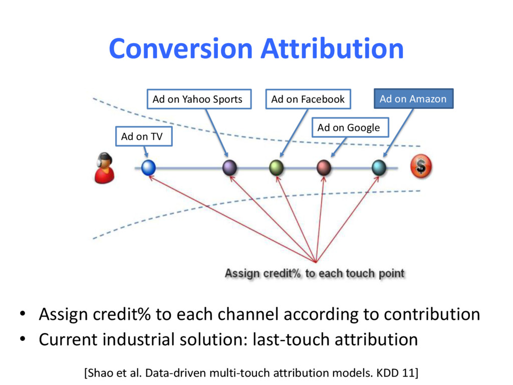
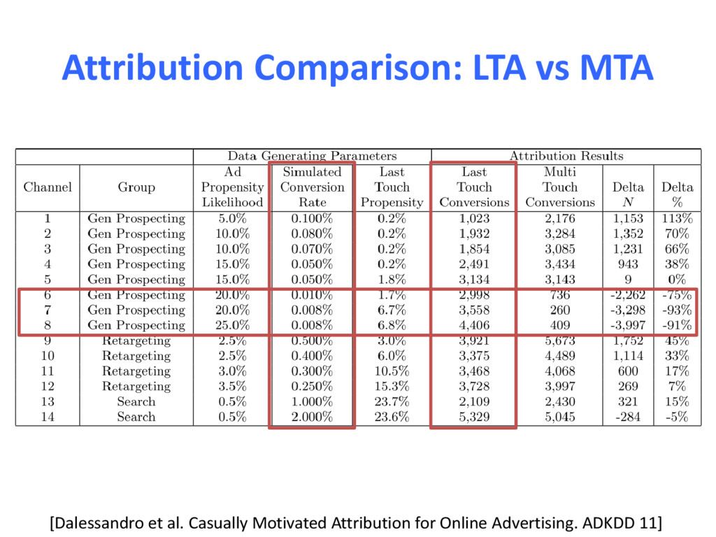
94. Conversion Attribution • Assign credit% to each channel according to contribution • Current industrial solution: last-touch attribution [Shao et al. Data-driven multi-touch attribution models. KDD 11] Ad on Yahoo Sports Ad on Facebook Ad on Amazon Ad on Google Ad on TV
95. Rule-based Attribution [Kee. Attribution playbook – google analytics. Online access.]
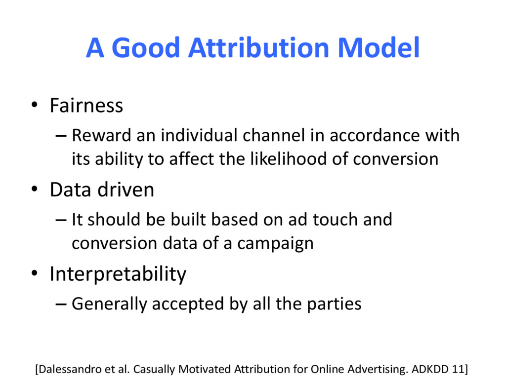
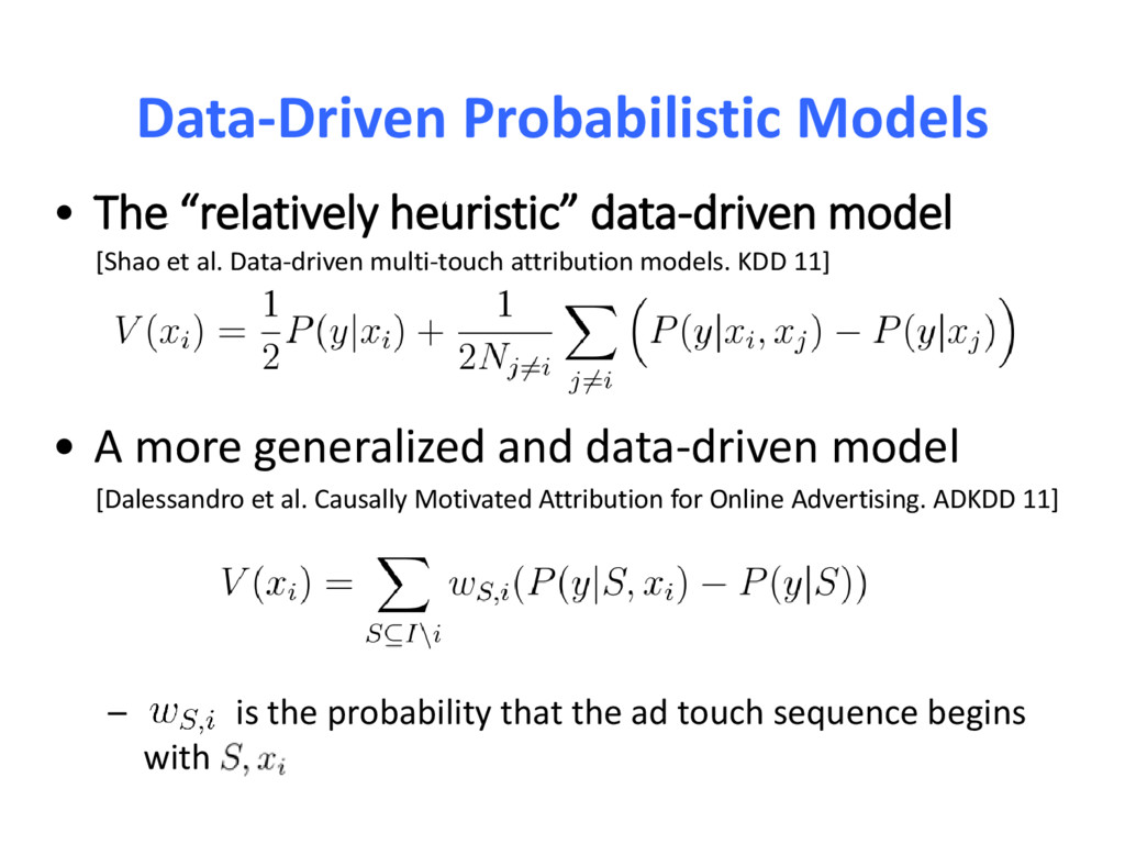
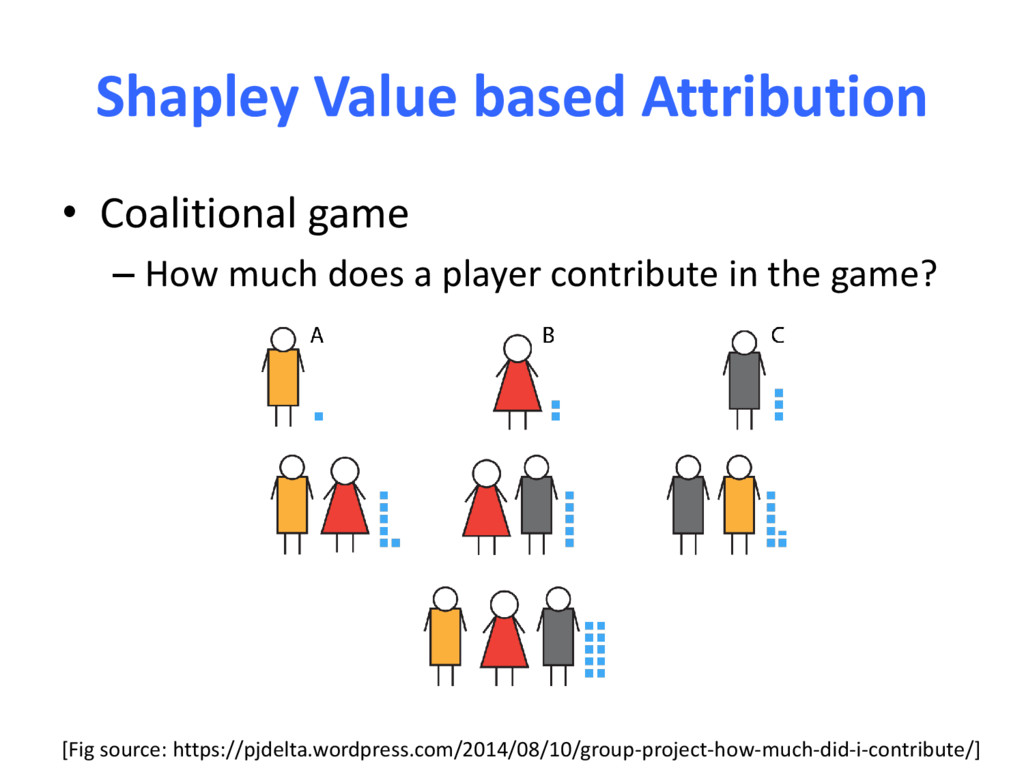
96. A Good Attribution Model • Fairness – Reward an individual channel in accordance with its ability to affect the likelihood of conversion • Data driven – It should be built based on ad touch and conversion data of a campaign • Interpretability – Generally accepted by all the parties [Dalessandro et al. Casually Motivated Attribution for Online Advertising. ADKDD 11]
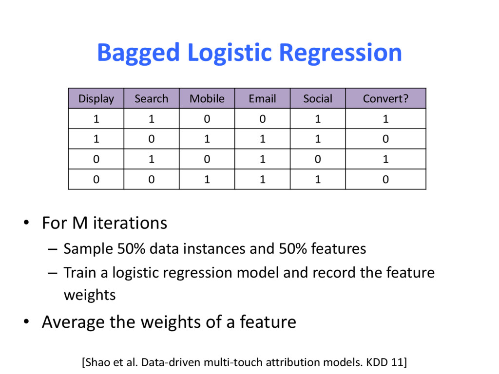
97. Bagged Logistic Regression • For M iterations – Sample 50% data instances and 50% features – Train a logistic regression model and record the feature weights • Average the weights of a feature Display Search Mobile Email Social Convert? 1 1 0 0 1 1 1 0 1 1 1 0 0 1 0 1 0 1 0 0 1 1 1 0 [Shao et al. Data-driven multi-touch attribution models. KDD 11]
98. A Probabilistic Attribution Model • Conditional probabilities • Attributed contribution (not-normalized) [Shao et al. Data-driven multi-touch attribution models. KDD 11]
99. [Shao et al. Data-driven multi-touch attribution models. KDD 11]
100. [Shao et al. Data-driven multi-touch attribution models. KDD 11]
101. Data-Driven Probabilistic Models [Shao et al. Data-driven multi-touch attribution models. KDD 11] • A more generalized and data-driven model [Dalessandro et al. Causally Motivated Attribution for Online Advertising. ADKDD 11] – is the probability that the ad touch sequence begins with • The “relatively heuristic” data-driven model
102. Attribution Comparison: LTA vs MTA [Dalessandro et al. Casually Motivated Attribution for Online Advertising. ADKDD 11]
103. Shapley Value based Attribution • Coalitional game – How much does a player contribute in the game? [Fig source: https://pjdelta.wordpress.com/2014/08/10/group-project-how-much-did-i-contribute/]
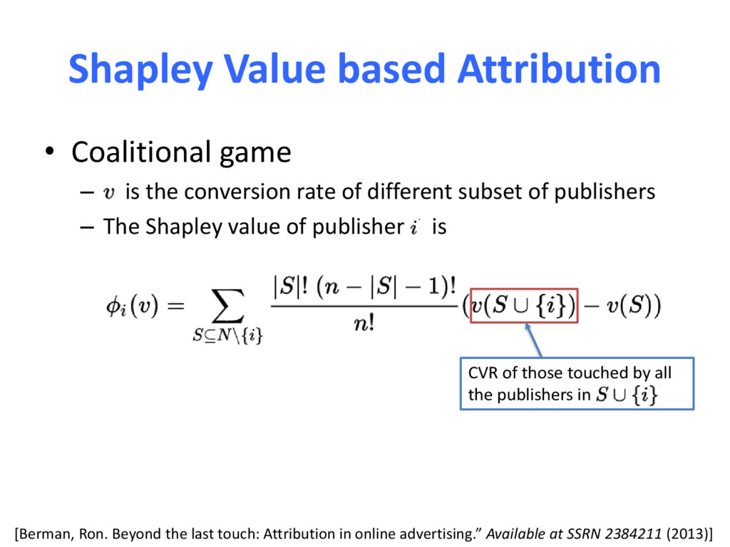
104. Shapley Value based Attribution • Coalitional game – is the conversion rate of different subset of publishers – The Shapley value of publisher is [Berman, Ron. Beyond the last touch: Attribution in online advertising.” Available at SSRN 2384211 (2013)] CVR of those touched by all the publishers in
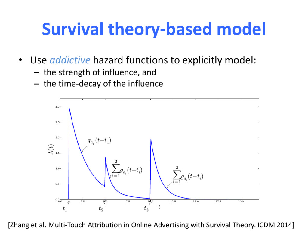
105. Survival theory-based model • Use addictive hazard functions to explicitly model: – the strength of influence, and – the time-decay of the influence [Zhang et al. Multi-Touch Attribution in Online Advertising with Survival Theory. ICDM 2014]
106. • Establish a graph from observed user journeys Markov graph-based approach [Anderl et al. Mapping the customer journey: A graph-based framework for online attribution modeling. SSRN 2014]
107. • Attribute based on probability change of reaching conversion state Markov graph-based approach [Anderl et al. Mapping the customer journey: A graph-based framework for online attribution modeling. SSRN 2014]
108. MTA-based budget allocation • Typical advertiser hierarchy • Typical budget allocation scheme [Geyik et al. Multi-Touch Attribution Based Budget Allocation in Online Advertising. ADKDD 14]
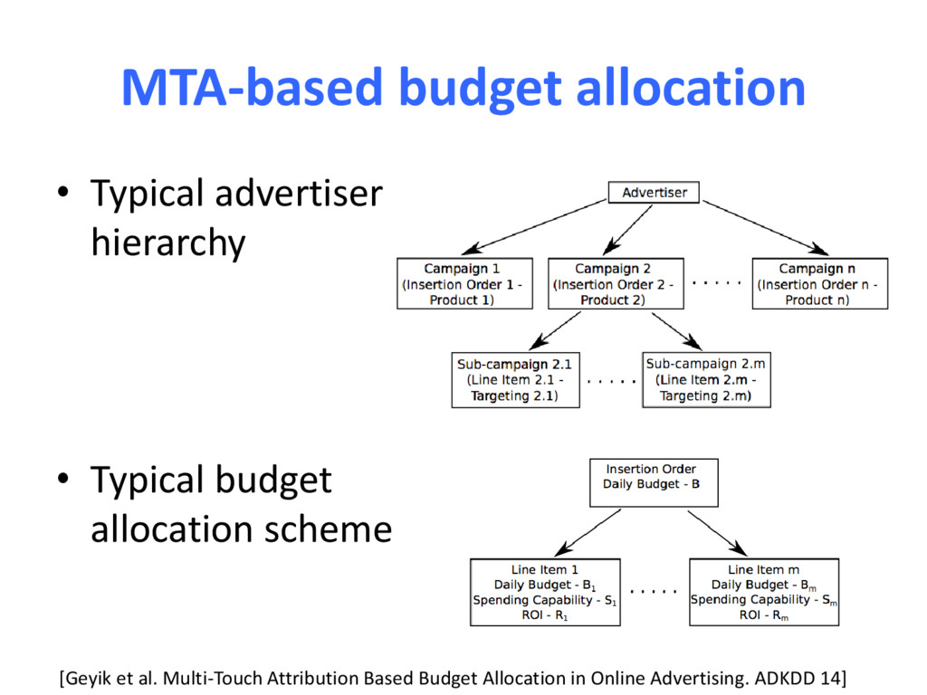
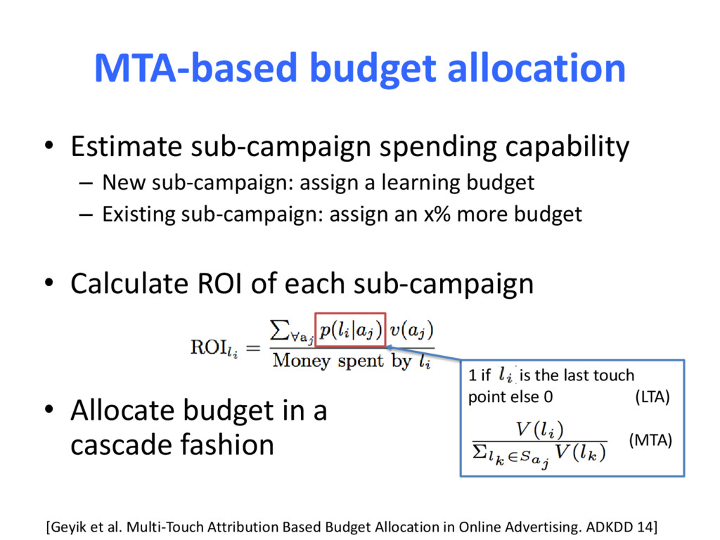
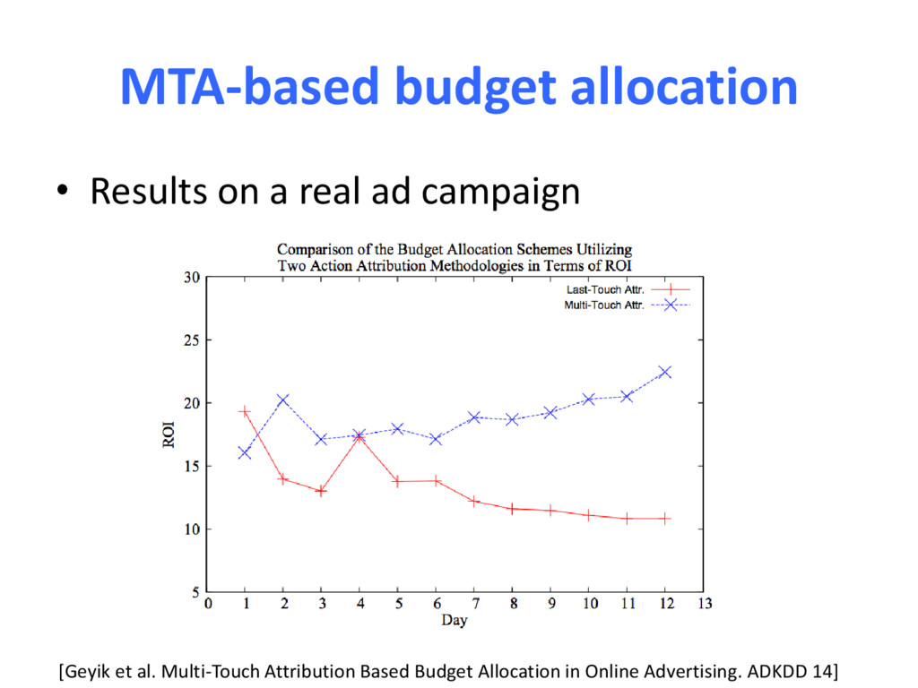
109. • Estimate sub-campaign spending capability – New sub-campaign: assign a learning budget – Existing sub-campaign: assign an x% more budget • Calculate ROI of each sub-campaign • Allocate budget in a cascade fashion 1 if is the last touch point else 0 (LTA) (MTA) MTA-based budget allocation [Geyik et al. Multi-Touch Attribution Based Budget Allocation in Online Advertising. ADKDD 14]
110. MTA-based budget allocation • Results on a real ad campaign [Geyik et al. Multi-Touch Attribution Based Budget Allocation in Online Advertising. ADKDD 14]
111. Attribution and Bidding • For CPA campaigns, conventional bidding strategy is to bid prop. to estimated action rate (a.k.a. conversion rate). Is that always correct? [Xu et al. Lift-Based Bidding in Ad Selection. AAAI 2016.]
112. Attribution and Bidding
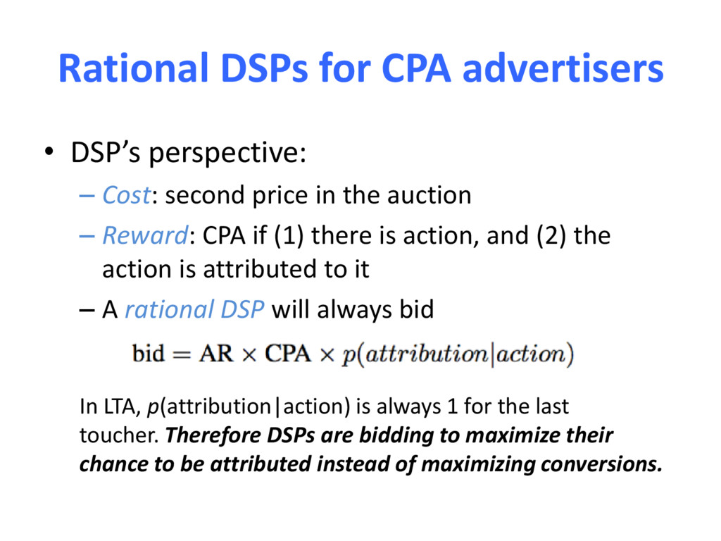
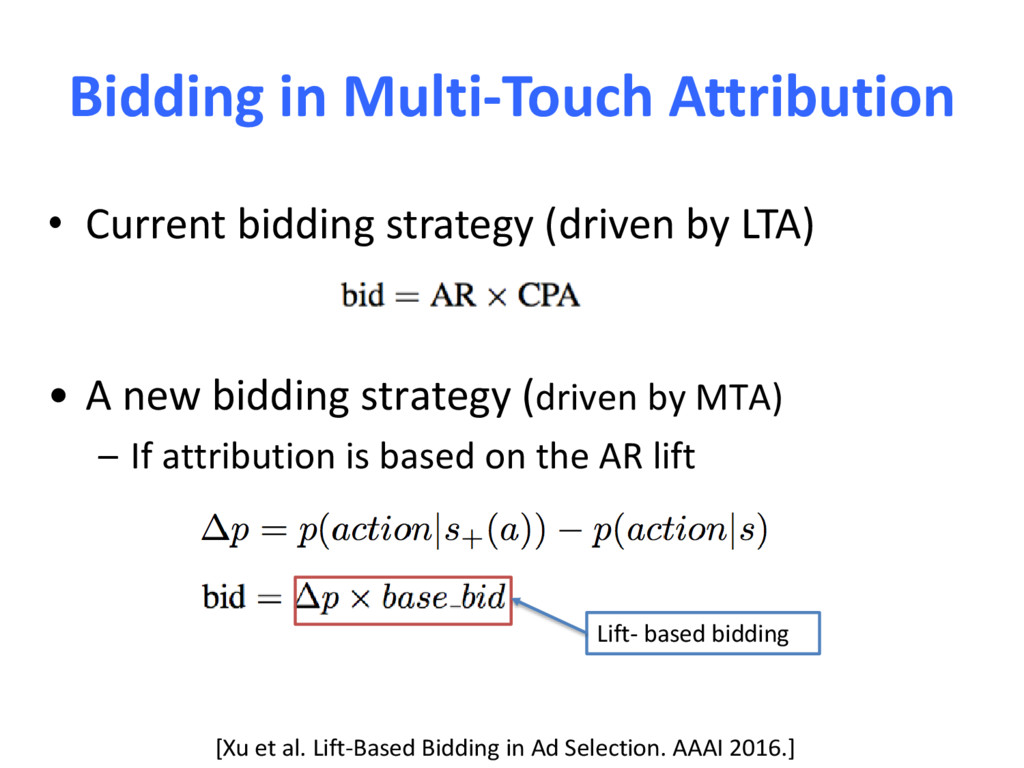
113. Rational DSPs for CPA advertisers • DSP’s perspective: – Cost: second price in the auction – Reward: CPA if (1) there is action, and (2) the action is attributed to it – A rational DSP will always bid In LTA, p(attribution|action) is always 1 for the last toucher. Therefore DSPs are bidding to maximize their chance to be attributed instead of maximizing conversions.
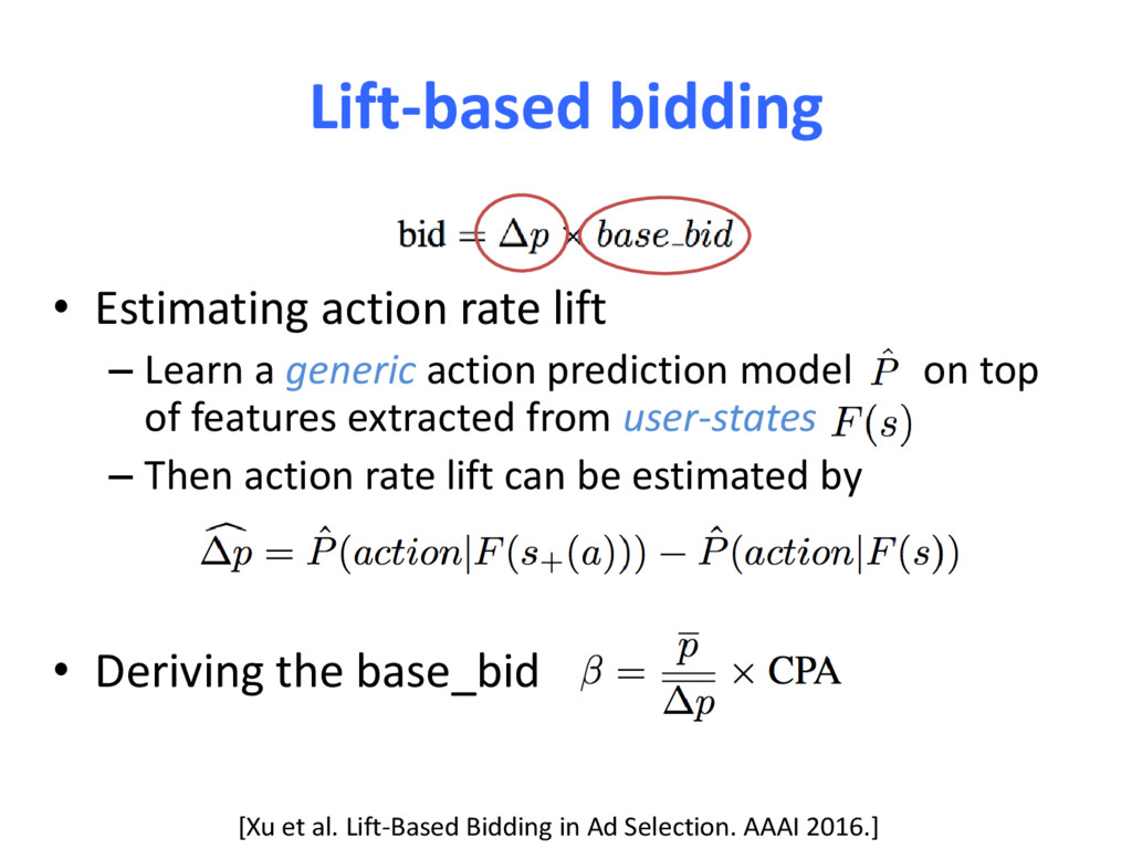
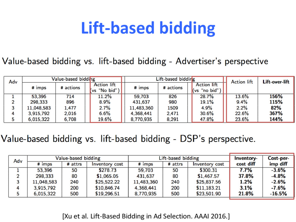
114. Bidding in Multi-Touch Attribution • Current bidding strategy (driven by LTA) • A new bidding strategy (driven by MTA) – If attribution is based on the AR lift [Xu et al. Lift-Based Bidding in Ad Selection. AAAI 2016.] Lift- based bidding
115. Lift-based bidding • Estimating action rate lift – Learn a generic action prediction model on top of features extracted from user-states – Then action rate lift can be estimated by • Deriving the base_bid [Xu et al. Lift-Based Bidding in Ad Selection. AAAI 2016.]
116. Lift-based bidding [Xu et al. Lift-Based Bidding in Ad Selection. AAAI 2016.]
117. Table of contents • RTB system • Auction mechanisms • User response estimation • Learning to bid • Conversion attribution • Pacing control • Targeting and audience expansion • Reserve price optimization
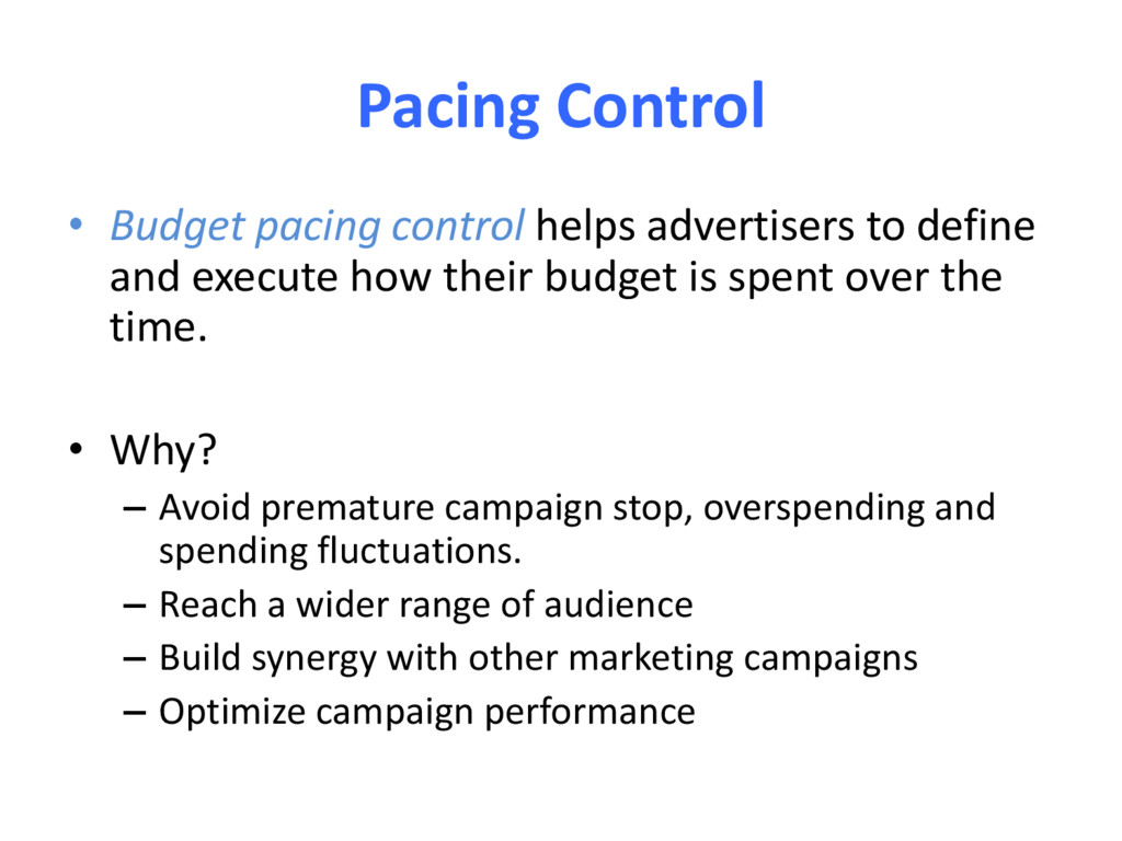
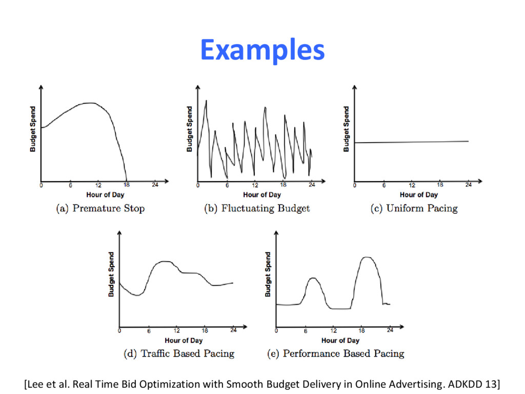
118. Pacing Control • Budget pacing control helps advertisers to define and execute how their budget is spent over the time. • Why? – Avoid premature campaign stop, overspending and spending fluctuations. – Reach a wider range of audience – Build synergy with other marketing campaigns – Optimize campaign performance
119. Examples [Lee et al. Real Time Bid Optimization with Smooth Budget Delivery in Online Advertising. ADKDD 13]
120. Two streams of approaches Bid modification Probabilistic throttling [Xu et al. Smart Pacing for Effective Online Ad Campaign Optimization. KDD 2015.]
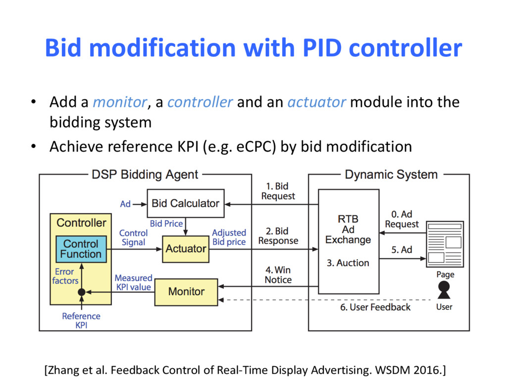
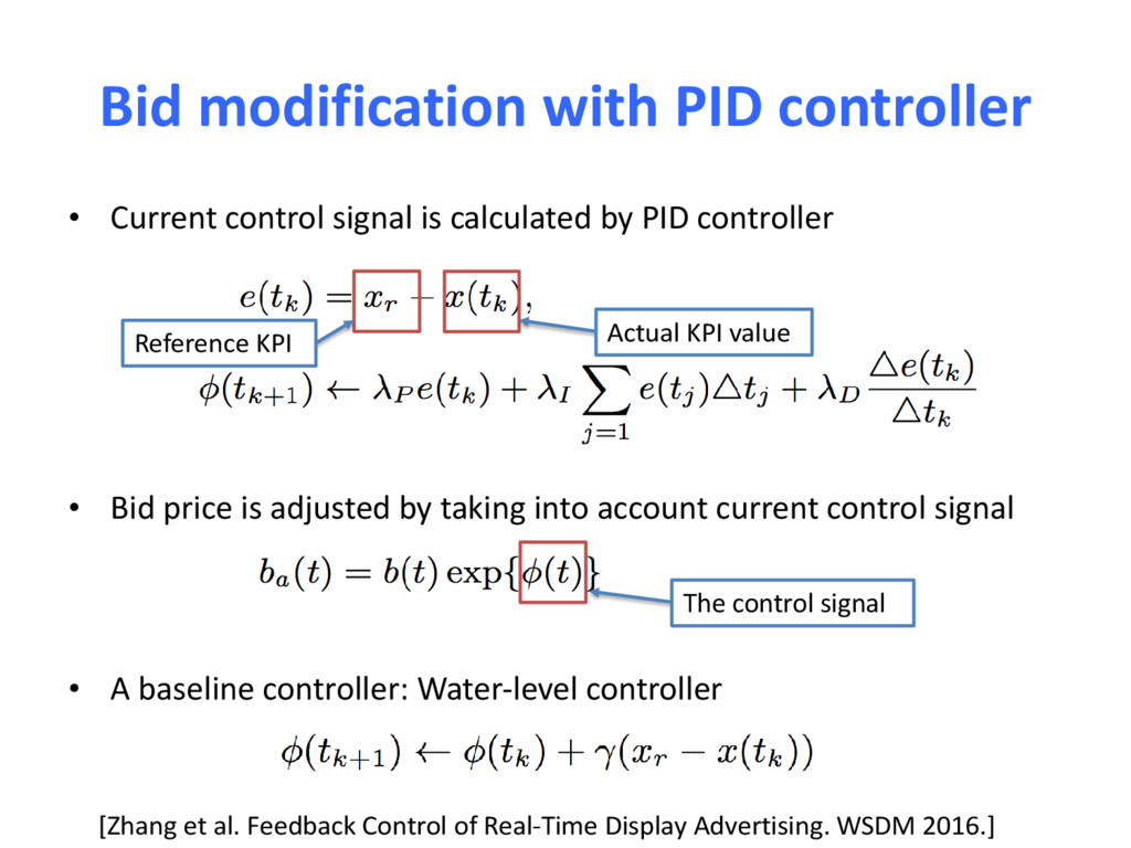
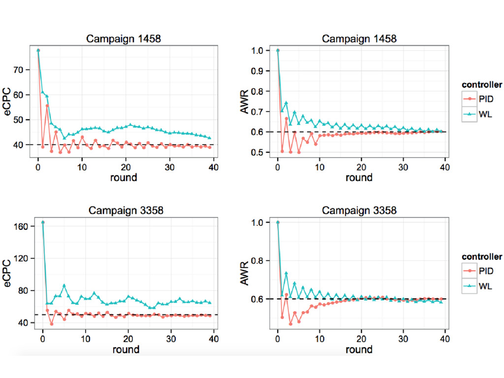
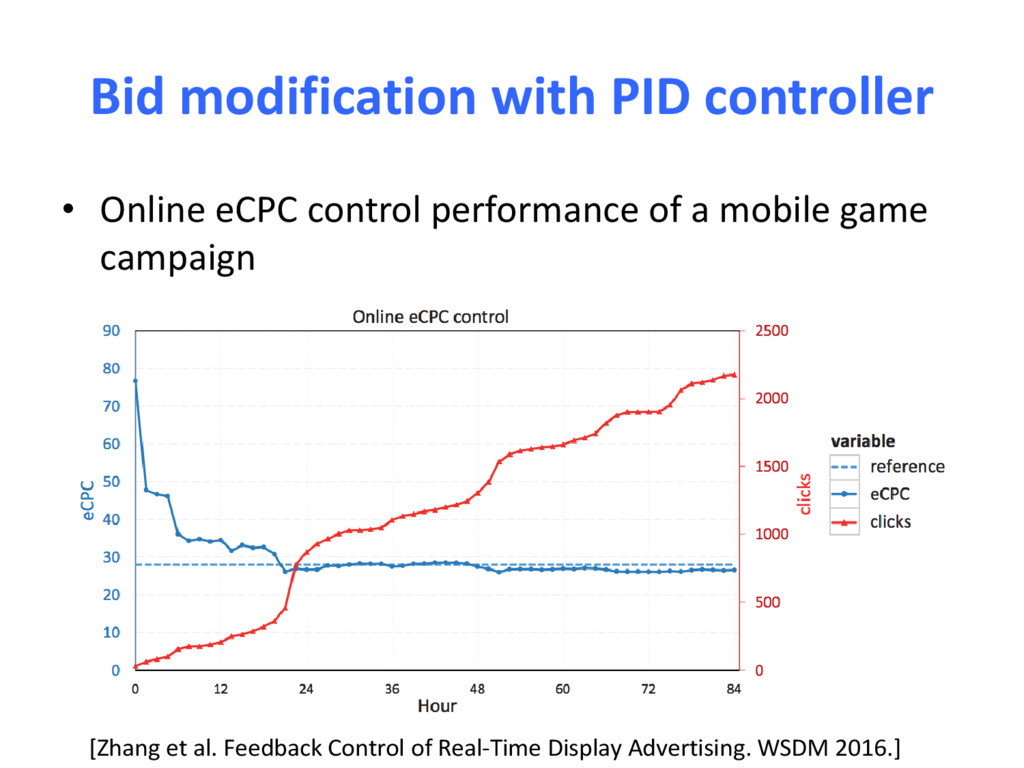
121. Bid modification with PID controller • Add a monitor, a controller and an actuator module into the bidding system • Achieve reference KPI (e.g. eCPC) by bid modification [Zhang et al. Feedback Control of Real-Time Display Advertising. WSDM 2016.]
122. Bid modification with PID controller • Current control signal is calculated by PID controller • Bid price is adjusted by taking into account current control signal • A baseline controller: Water-level controller [Zhang et al. Feedback Control of Real-Time Display Advertising. WSDM 2016.] The control signal Reference KPI Actual KPI value
124. • Online eCPC control performance of a mobile game campaign Bid modification with PID controller [Zhang et al. Feedback Control of Real-Time Display Advertising. WSDM 2016.]
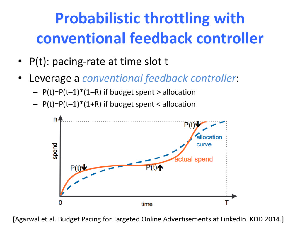
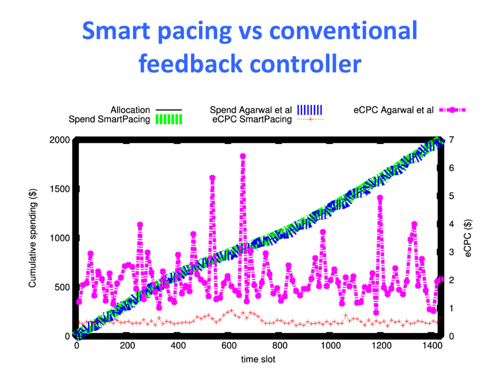
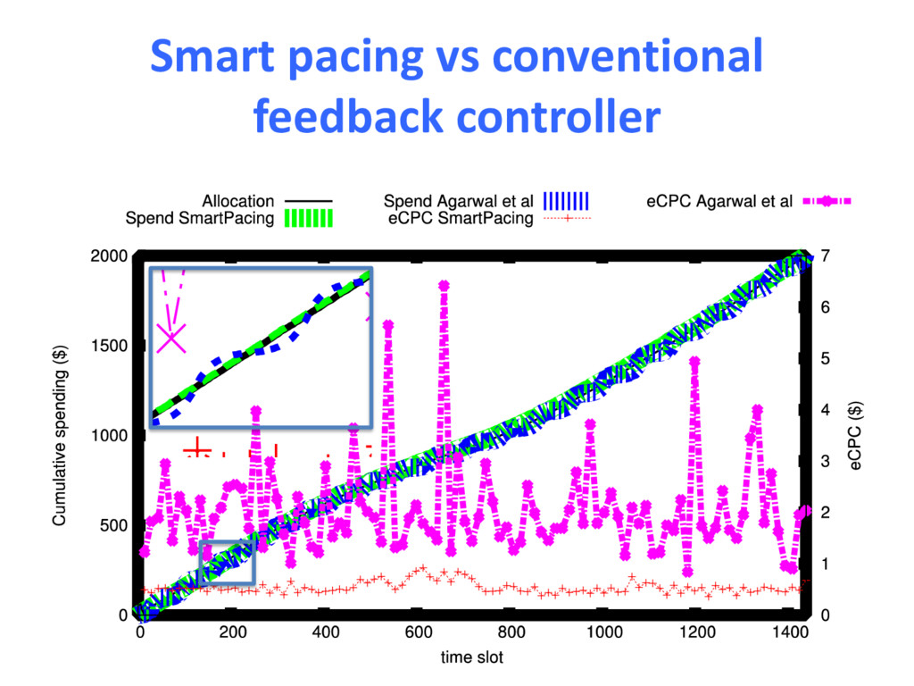
125. Probabilistic throttling with conventional feedback controller • P(t): pacing-rate at time slot t • Leverage a conventional feedback controller: – P(t)=P(t–1)*(1–R) if budget spent > allocation – P(t)=P(t–1)*(1+R) if budget spent < allocation [Agarwal et al. Budget Pacing for Targeted Online Advertisements at LinkedIn. KDD 2014.]
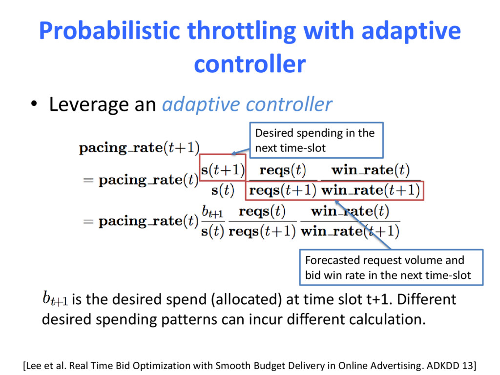
126. Probabilistic throttling with adaptive controller • Leverage an adaptive controller is the desired spend (allocated) at time slot t+1. Different desired spending patterns can incur different calculation. [Lee et al. Real Time Bid Optimization with Smooth Budget Delivery in Online Advertising. ADKDD 13] Desired spending in the next time-slot Forecasted request volume and bid win rate in the next time-slot
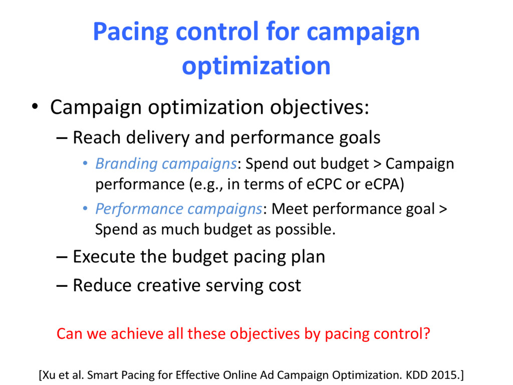
127. Pacing control for campaign optimization • Campaign optimization objectives: – Reach delivery and performance goals • Branding campaigns: Spend out budget > Campaign performance (e.g., in terms of eCPC or eCPA) • Performance campaigns: Meet performance goal > Spend as much budget as possible. – Execute the budget pacing plan – Reduce creative serving cost Can we achieve all these objectives by pacing control? [Xu et al. Smart Pacing for Effective Online Ad Campaign Optimization. KDD 2015.]
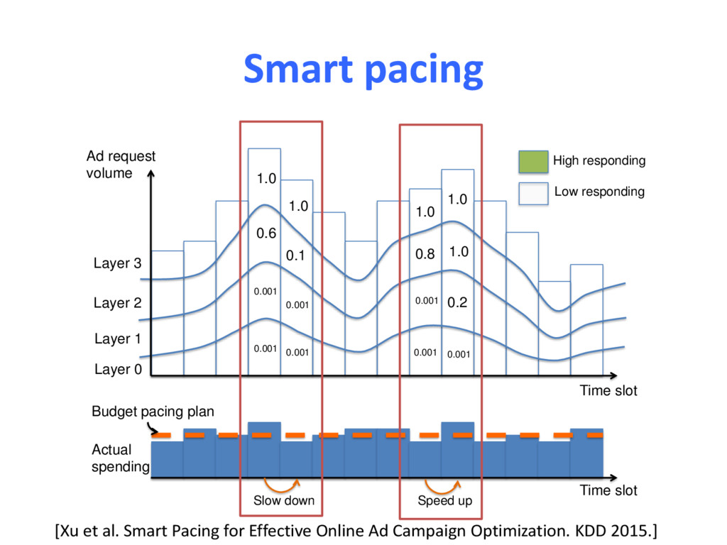
128. Smart pacing 1.0 0.6 1.0 0.1 0.001 0.001 0.001 0.001 1.0 1.0 0.8 1.0 0.001 0.2 Layer 3 Layer 2 Layer 1 Layer 0 Ad request volume Time slot Budget pacing plan Actual spending Time slot High responding Low responding 0.001 0.001 Slow down Speed up [Xu et al. Smart Pacing for Effective Online Ad Campaign Optimization. KDD 2015.]
129. Smart pacing performance
130. Smart pacing vs conventional feedback controller
131. Smart pacing vs conventional feedback controller
132. Table of contents • RTB system • Auction mechanisms • User response estimation • Learning to bid • Conversion attribution • Pacing control • Targeting and audience expansion • Reserve price optimization
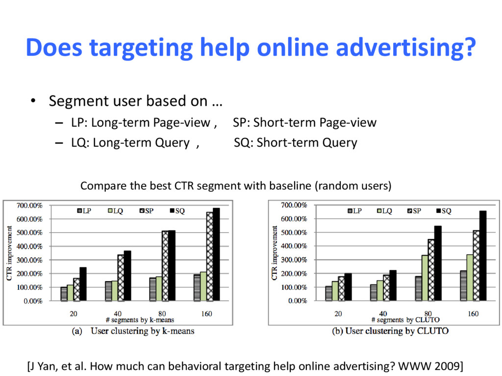
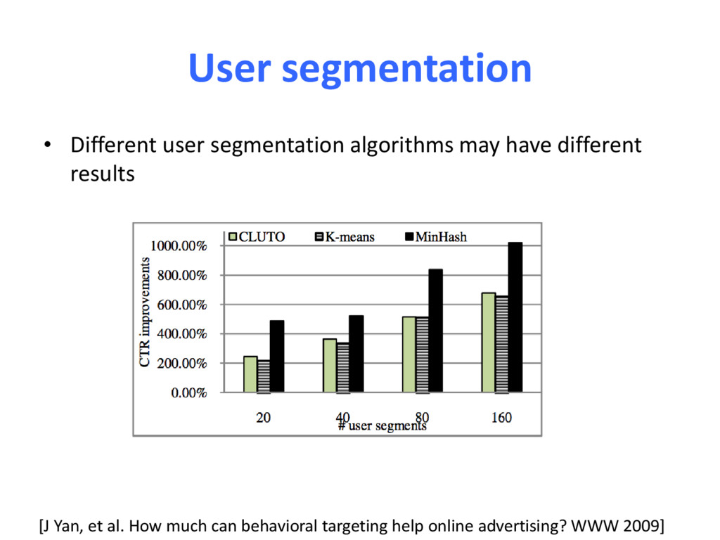
133. Does targeting help online advertising? • Segment user based on … – LP: Long-term Page-view , SP: Short-term Page-view – LQ: Long-term Query , SQ: Short-term Query [J Yan, et al. How much can behavioral targeting help online advertising? WWW 2009] Compare the best CTR segment with baseline (random users)
134. User segmentation • Different user segmentation algorithms may have different results [J Yan, et al. How much can behavioral targeting help online advertising? WWW 2009]
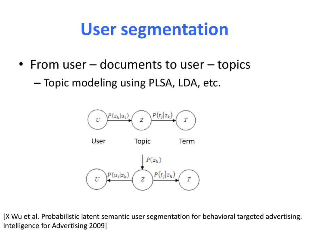
135. User segmentation • From user – documents to user – topics – Topic modeling using PLSA, LDA, etc. [X Wu et al. Probabilistic latent semantic user segmentation for behavioral targeted advertising. Intelligence for Advertising 2009] User Topic Term
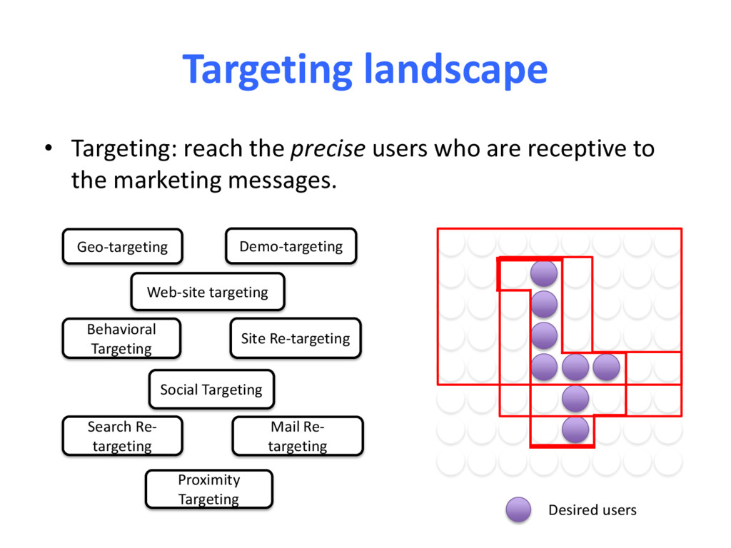
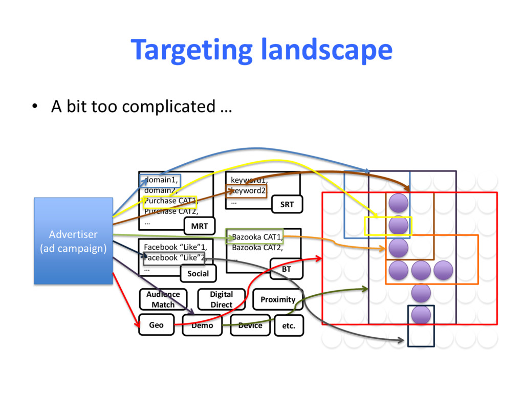
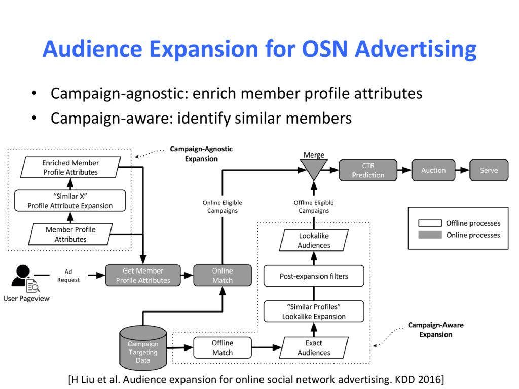
136. Targeting landscape • Targeting: reach the precise users who are receptive to the marketing messages. Geo-targeting Demo-targeting Behavioral Targeting Search Re- targeting Mail Re- targeting Social Targeting Site Re-targeting Desired users Web-site targeting Proximity Targeting
137. Targeting landscape • A bit too complicated … domain1, domain2, Purchase CAT1, Purchase CAT2, … MRT keyword1, keyword2, … SRT Facebook “Like”1, Facebook “Like”2, … Social Bazooka CAT1, Bazooka CAT2, … BT Audience Match Digital Direct Proximity Geo Demo Device Advertiser (ad campaign) etc.
138. Audience expansion • AEX Simplifies targeting by discovering similar (prospective) customers [J Shen, et al., Effective Audience Extension in Online Advertising, KDD 2015]
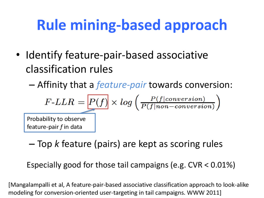
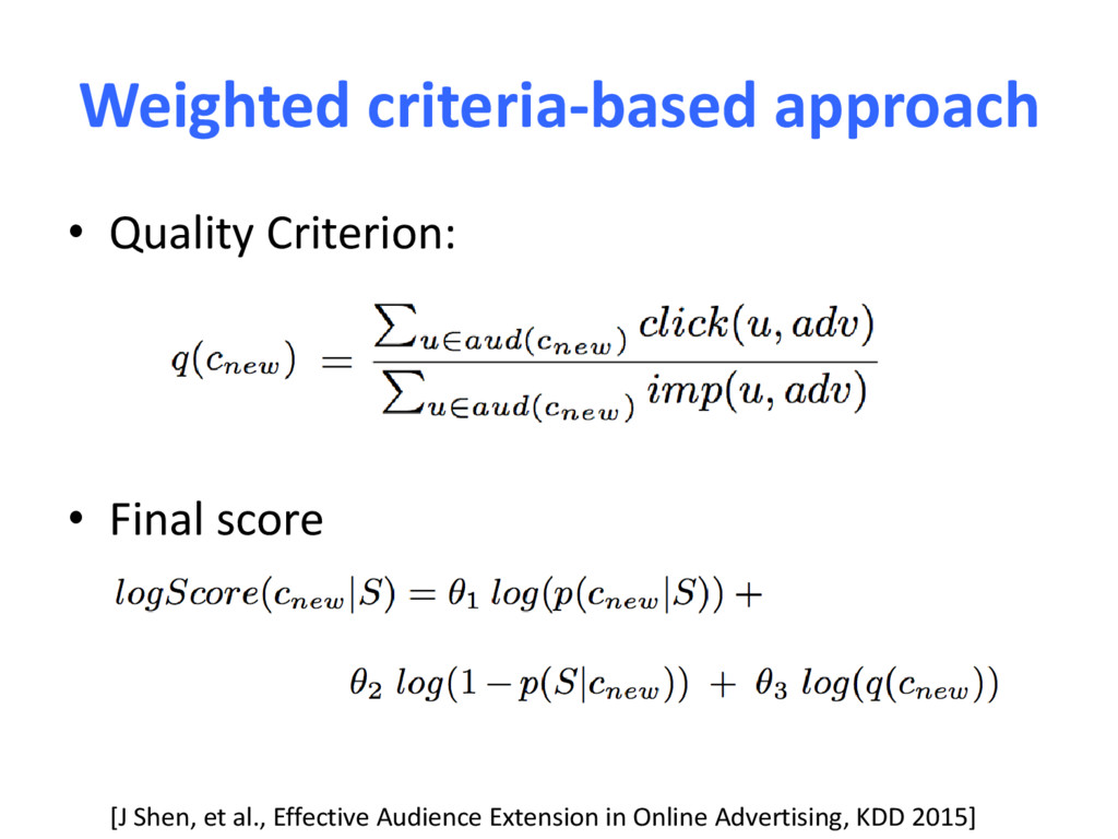
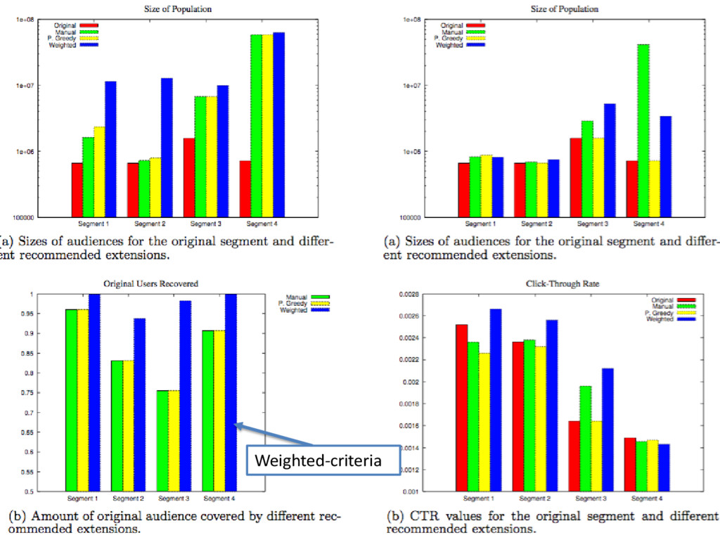
139. Rule mining-based approach • Identify feature-pair-based associative classification rules – Affinity that a feature-pair towards conversion: – Top k feature (pairs) are kept as scoring rules Especially good for those tail campaigns (e.g. CVR < 0.01%) [Mangalampalli et al, A feature-pair-based associative classification approach to look-alike modeling for conversion-oriented user-targeting in tail campaigns. WWW 2011] Probability to observe feature-pair f in data
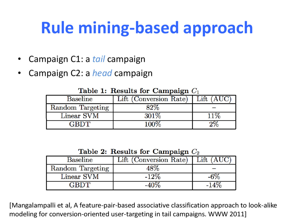
140. Rule mining-based approach • Campaign C1: a tail campaign • Campaign C2: a head campaign [Mangalampalli et al, A feature-pair-based associative classification approach to look-alike modeling for conversion-oriented user-targeting in tail campaigns. WWW 2011]
141. Weighted criteria-based approach • Similarity Criterion: • Novelty Criterion: [J Shen, et al., Effective Audience Extension in Online Advertising, KDD 2015]
142. Weighted criteria-based approach • Quality Criterion: • Final score [J Shen, et al., Effective Audience Extension in Online Advertising, KDD 2015]
143. Weighted criteria-based approach Weighted-criteria
144. Audience Expansion for OSN Advertising • Campaign-agnostic: enrich member profile attributes • Campaign-aware: identify similar members [H Liu et al. Audience expansion for online social network advertising. KDD 2016]
145. Audience Expansion for OSN Advertising • Member similarity evaluation – Density of a segment: – Expansion ratio vs Density ratio [H Liu et al. Audience expansion for online social network advertising. KDD 2016]
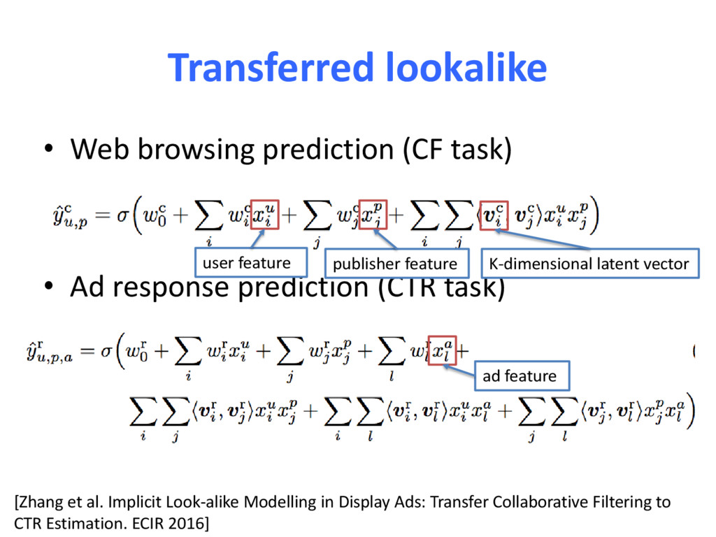
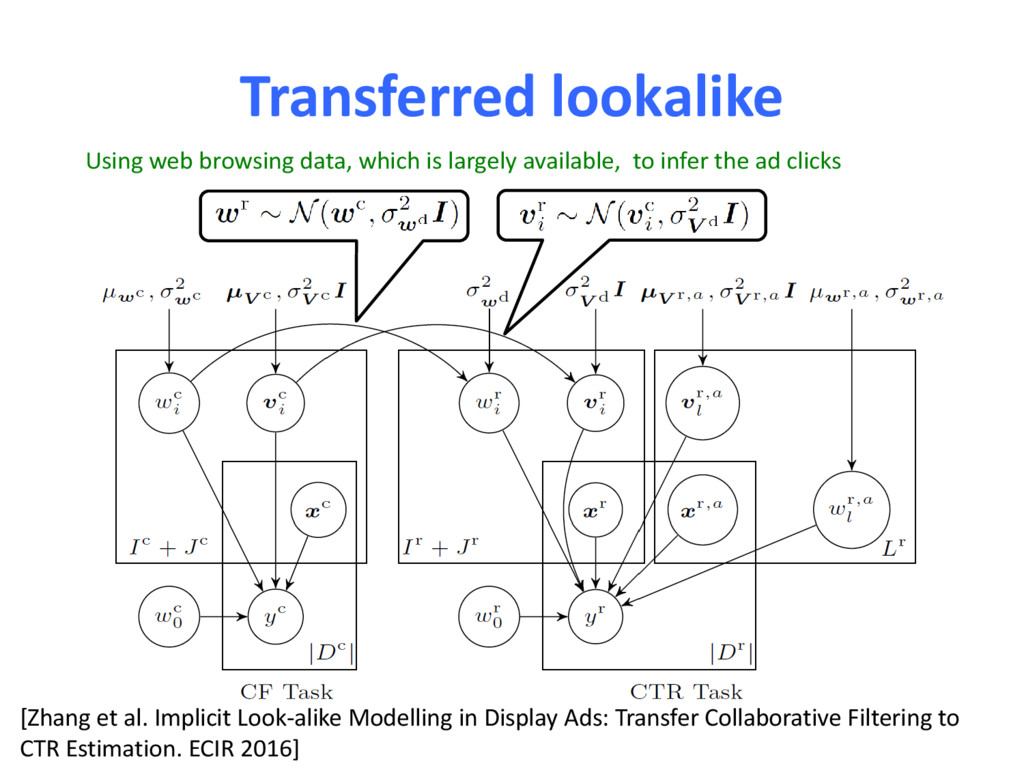
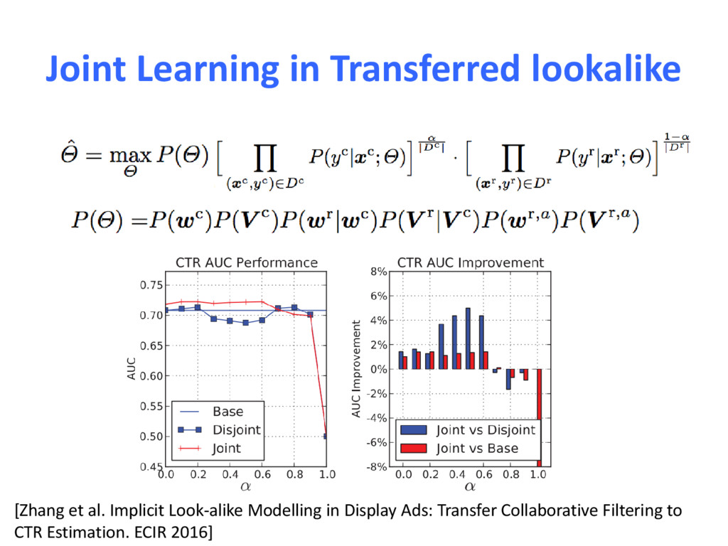
146. Transferred lookalike • Web browsing prediction (CF task) • Ad response prediction (CTR task) [Zhang et al. Implicit Look-alike Modelling in Display Ads: Transfer Collaborative Filtering to CTR Estimation. ECIR 2016] user feature publisher feature K-dimensional latent vector ad feature
147. Transferred lookalike Using web browsing data, which is largely available, to infer the ad clicks [Zhang et al. Implicit Look-alike Modelling in Display Ads: Transfer Collaborative Filtering to CTR Estimation. ECIR 2016]
148. Joint Learning in Transferred lookalike [Zhang et al. Implicit Look-alike Modelling in Display Ads: Transfer Collaborative Filtering to CTR Estimation. ECIR 2016]
149. Table of contents • RTB system • Auction mechanisms • User response estimation • Learning to bid • Conversion attribution • Pacing control • Targeting and audience expansion • Reserve price optimization
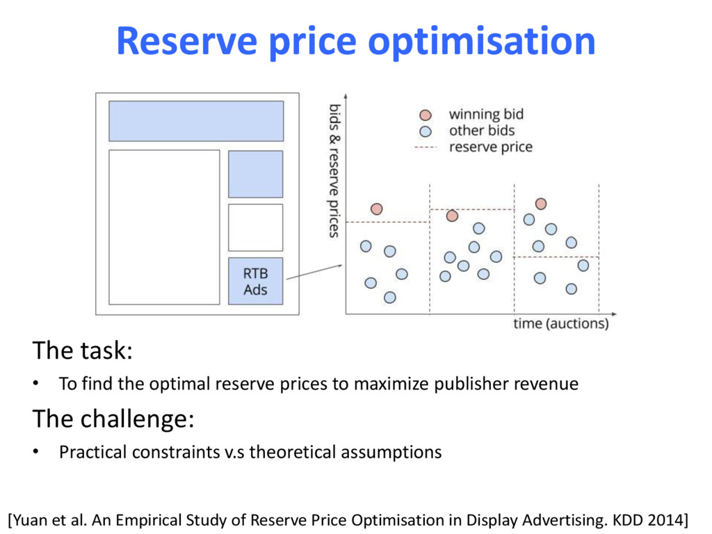
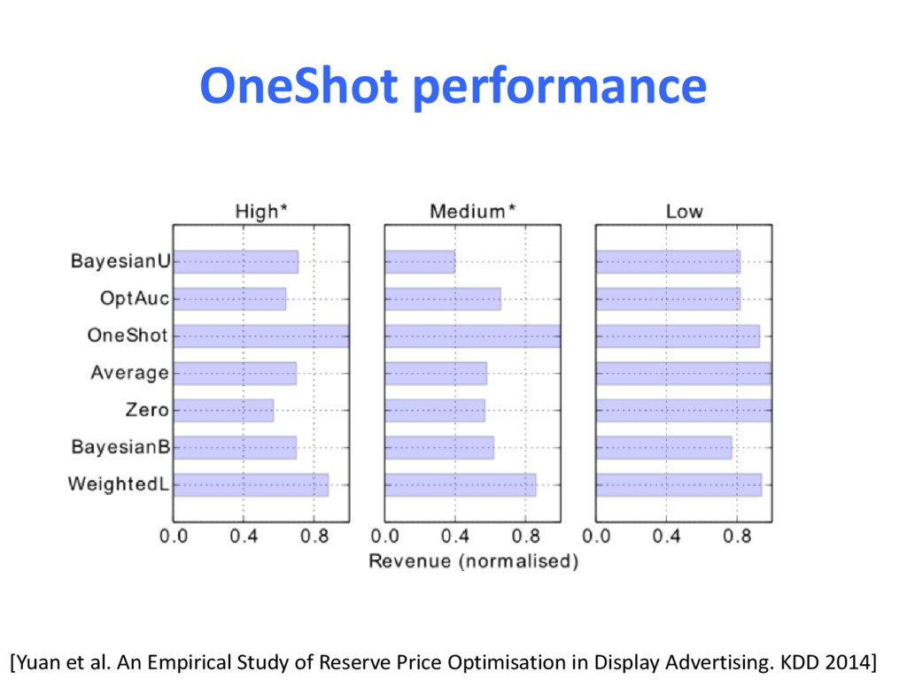
150. Reserve price optimisation The task: • To find the optimal reserve prices to maximize publisher revenue The challenge: • Practical constraints v.s theoretical assumptions [Yuan et al. An Empirical Study of Reserve Price Optimisation in Display Advertising. KDD 2014]
151. Why • Suppose it is second price auction and 1 , 2 are first and second prices – Preferable case: 1 ≥ > 2 (increases revenue) – Undesirable case: > 1 (lose revenue)
152. • Suppose: two bidders, whose private values 1 , 2 are both drawn from Uniform[0, 1] • Without a reserve price, the expected payoff is: • With α = 0.2: • With α = 0.5: • With α = 0.6: An example [Ostrovsky et al, Reserve prices in internet advertising auctions: A field experiment. EC 2011] = min 1 , 2 = 0.33 = min 1 , 2 1 > 0.5, 2 > 0.5 + (0.5 × 0.5) × 2 × 0.5 = 0.42 = min 1 , 2 1 > 0.2, 2 > 0.2 + (0.8 × 0.2) × 2 × 0.2 = 0.36 = min 1 , 2 1 > 0.6, 2 > 0.6 + 0.6 × 0.4 × 2 × 0.6 = 0.405 Paying the second highest price Paying the reserve price
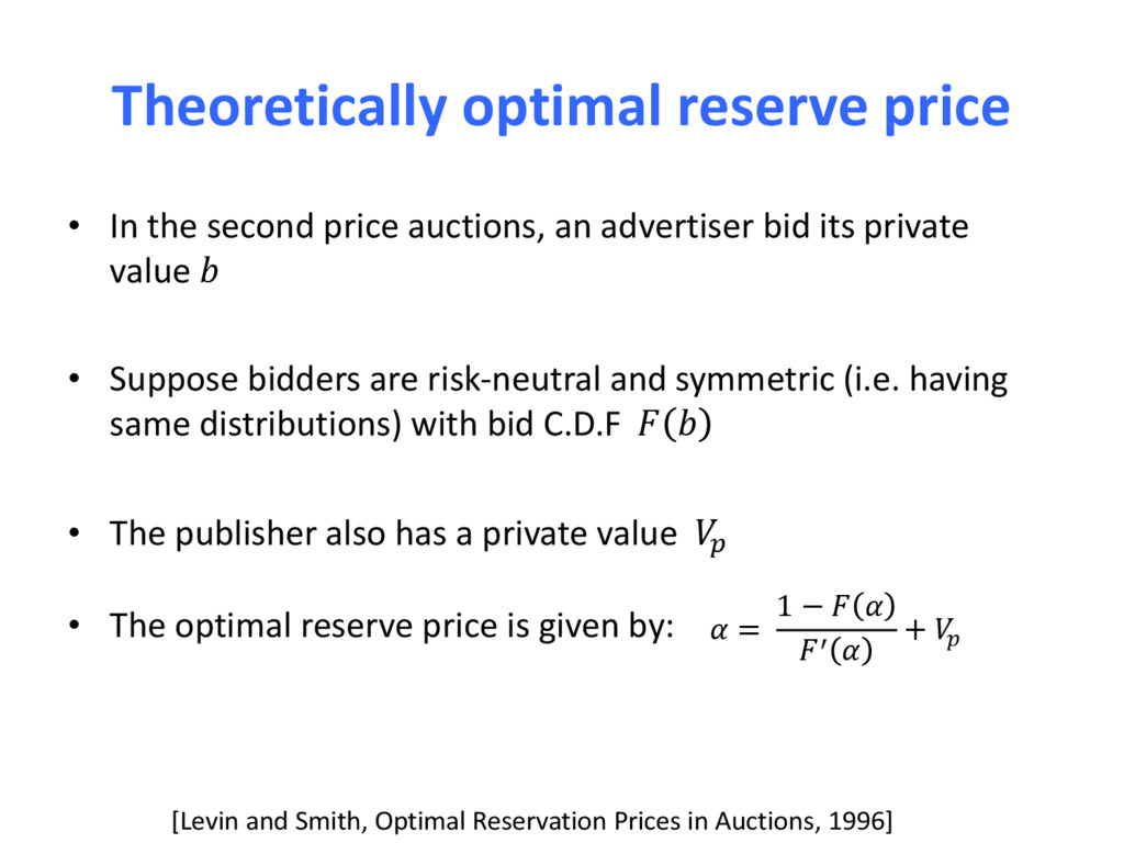
153. Theoretically optimal reserve price • In the second price auctions, an advertiser bid its private value • Suppose bidders are risk-neutral and symmetric (i.e. having same distributions) with bid C.D.F • The publisher also has a private value • The optimal reserve price is given by: [Levin and Smith, Optimal Reservation Prices in Auctions, 1996] = 1 − ′ +
154. Results from a field experiment • Using the theoretically optimal reserve price on Yahoo! Sponsored search Mixed results [Ostrovsky et al, Reserve prices in internet advertising auctions: A field experiment. EC 2011]
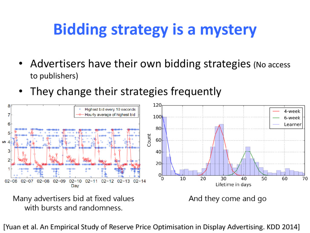
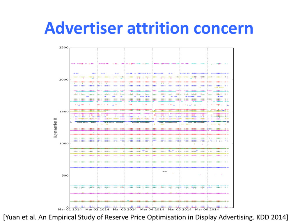
155. • Advertisers have their own bidding strategies (No access to publishers) • They change their strategies frequently Bidding strategy is a mystery Many advertisers bid at fixed values with bursts and randomness. And they come and go [Yuan et al. An Empirical Study of Reserve Price Optimisation in Display Advertising. KDD 2014]
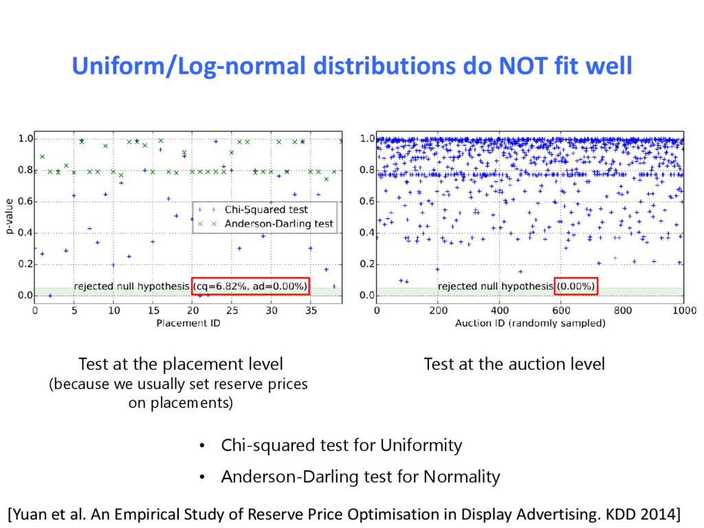
156. Uniform/Log-normal distributions do NOT fit well Test at the placement level (because we usually set reserve prices on placements) Test at the auction level • Chi-squared test for Uniformity • Anderson-Darling test for Normality [Yuan et al. An Empirical Study of Reserve Price Optimisation in Display Advertising. KDD 2014]
157. A simplified dynamic game • Players: auction winner ,publisher • Initial status: : ; otherwise [Yuan et al. An Empirical Study of Reserve Price Optimisation in Display Advertising. KDD 2014]
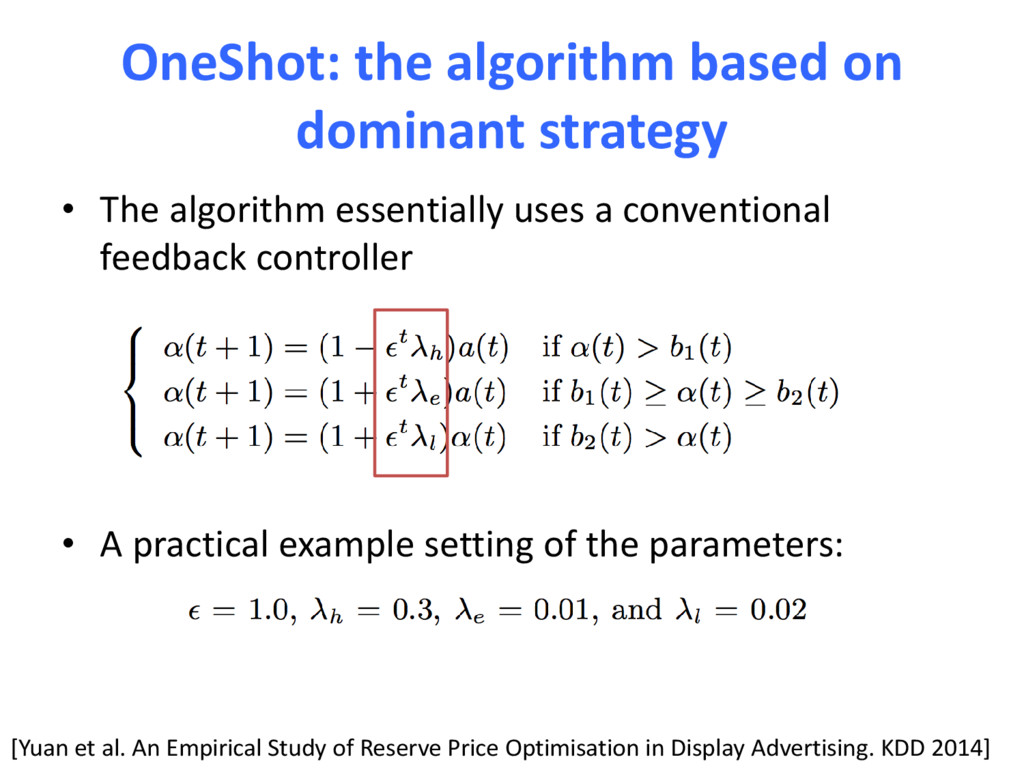
158. OneShot: the algorithm based on dominant strategy • The algorithm essentially uses a conventional feedback controller • A practical example setting of the parameters: [Yuan et al. An Empirical Study of Reserve Price Optimisation in Display Advertising. KDD 2014]
159. OneShot performance [Yuan et al. An Empirical Study of Reserve Price Optimisation in Display Advertising. KDD 2014]
160. [Yuan et al. An Empirical Study of Reserve Price Optimisation in Display Advertising. KDD 2014] Advertiser attrition concern
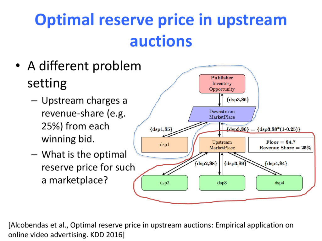
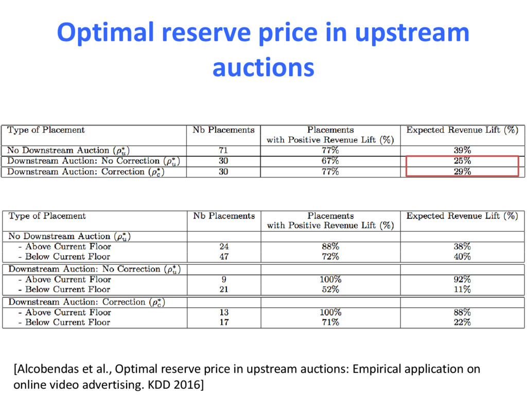
161. Optimal reserve price in upstream auctions • A different problem setting – Upstream charges a revenue-share (e.g. 25%) from each winning bid. – What is the optimal reserve price for such a marketplace? [Alcobendas et al., Optimal reserve price in upstream auctions: Empirical application on online video advertising. KDD 2016]
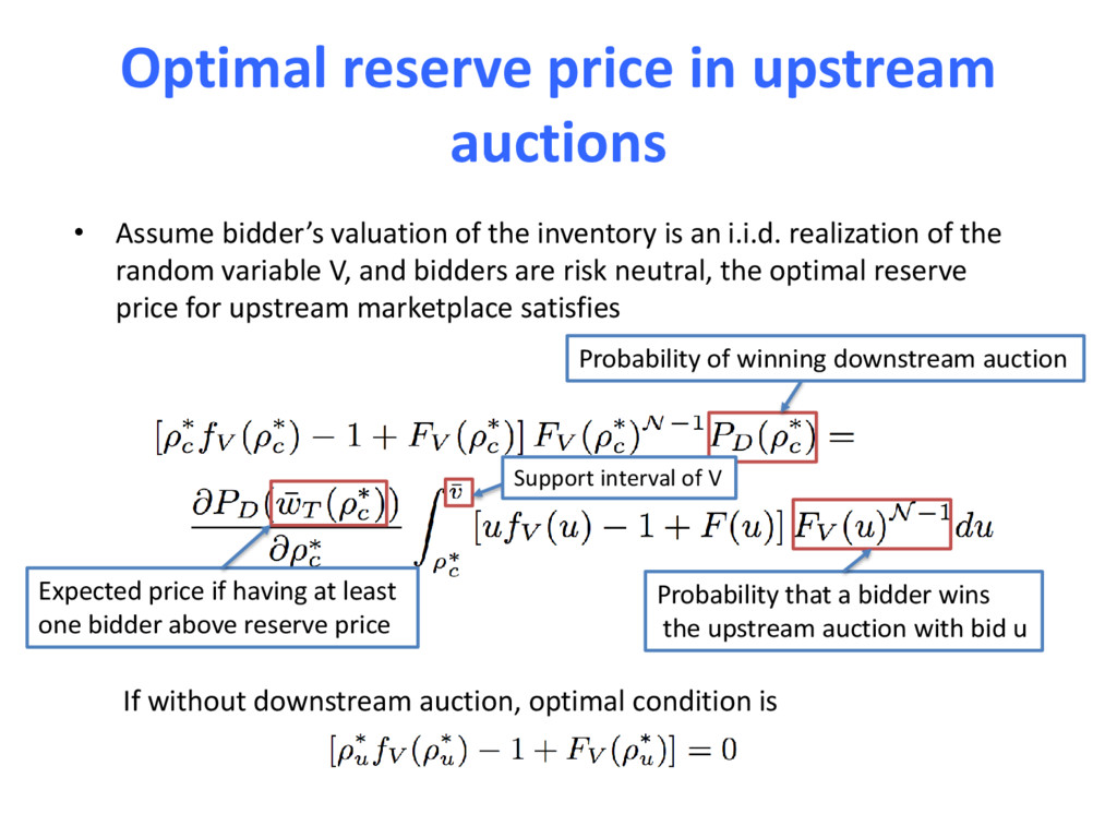
162. Optimal reserve price in upstream auctions • Assume bidder’s valuation of the inventory is an i.i.d. realization of the random variable V, and bidders are risk neutral, the optimal reserve price for upstream marketplace satisfies If without downstream auction, optimal condition is Probability of winning downstream auction Probability that a bidder wins the upstream auction with bid u Expected price if having at least one bidder above reserve price Support interval of V
163. Optimal reserve price in upstream auctions [Alcobendas et al., Optimal reserve price in upstream auctions: Empirical application on online video advertising. KDD 2016]
164. Thank You • RTB system • Auction mechanisms • User response estimation • Learning to bid • Conversion attribution • Pacing control • Targeting and audience expansion • Reserve price optimization Learning, Prediction and Optimisation in RTB Display Advertising Weinan Zhang (wnzhang AT sjtu.edu.cn) Jian Xu (jian.xu AT cootek.cn) CIKM16 Tutorial