Upgrade to Pro — share decks privately, control downloads, hide ads and more …

Quasi-Monte Carlo and Combinatorial Discrepancy...

Avatar for Nathan Kirk Nathan Kirk
November 11, 2025
6

Quasi-Monte Carlo and Combinatorial Discrepancy (Nov 2025)

Talk given at:
- Department of Statistics and Actuarial Sciences, Statistics Seminar at the University of Waterloo on Nov 11th, 2025
- Department of Applied Mathematics, Computational Mathematics Seminar at Illinois Institute of Technology on Nov 20th, 2025

NB: There are several animations that do not play in Speaker Deck versions of the slides.
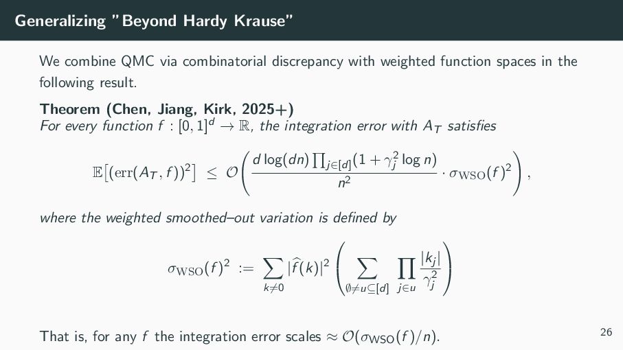
Avatar for Nathan Kirk

Nathan Kirk

November 11, 2025
Tweet

Transcript

  1. Quasi-Monte Carlo and Combinatorial Discrepancy Improved Error Bounds and a

    QMC Construction Dr. Nathan Kirk November 20th, 2025 Department of Applied Mathematics Illinois Tech
  2. Outline • Monte Carlo and quasi-Monte Carlo methods • A

    recent method of H. Jiang (U. Chicago) and N. Bansal (U. Michigan); QMC via combinatorial discrepancy • Extensions to high-dimensional integration • Summary Talk based on ”High-dimensional Quasi-Monte Carlo via Combinatorial Discrepancy” (arXiv, 2508.18426), joint work with J. Chen and H. Jiang (University of Chicago). 1
  3. Our Problem We examine the problem of numerically estimating the

    integral of a d−dimensional function f : [0, 1]d → R: I = [0,1]d f (x) dx. Integrals of this kind appear across finance, engineering, computer science, probability and robotics to name a few. Exact computation often impossible if f lacks a closed form anti-derivative, or we have only query access to f . Thus, numerical methods are required to accurately approximate I. Monte Carlo methods (and variants) are a popular choice. 2
  4. The Monte Carlo method – Illustrative Example Let’s consider a

    one-dimensional toy function f (x) = 1 + x2 + 1 2 sin(4πx). Our goal is to estimate the shaded area, 1 0 f (x) dx = 4/3 = 1.3333... 3
  5. The Monte Carlo method Our goal is to estimate I

    = [0,1]d f (x) dx. Monte Carlo Procedure: 1. Sample the domain [0, 1]d uniformly at random n times to obtain X1, X2, . . . , Xn 2. Compute f (Xi ) for each i 3. Compute the sample mean: IMC = 1 N n i=1 f (Xi ). Accuracy: The error ϵ := ˆ IMC − I scales as σ(f )/ √ n OR n ≈ (σ(f ))2/ϵ2. f may be expensive, or runtime may be an issue ⇒ Can we use less samples? 4
  6. The quasi-Monte Carlo method Quasi-Monte Carlo Procedure: 1. replace random

    samples by low-discrepancy (LD)–or evenly spread–points X1, . . . , Xn ∈ [0, 1]d . 2. Compute f (Xi ) of each i 3. Compute the sample mean to obtain ˆ IQMC. Accuracy: The deterministic QMC error is improved to O(1/n). 5
  7. The quasi-Monte Carlo method - An Example Using the same

    one-dimensional example with low-discrepancy sampling... 6
  8. QMC Key Idea QMC error analysis begins with the Hlawka-Zaremba

    formula: Error ϵ := |ˆ I − I| = 1 n 1 0 D(x) · f ′(x) dx (in one-dimension), where D(x) = nx − |X ∩ [0, x)| is the (local) continuous discrepancy of [0, x). Using the Cauchy-Schwarz inequality: Error ϵ ≤ 1 n 1 0 D(x)2 dx 1/2 · 1 0 f ′(x)2 dx 1/2 Koksma-Hlawka Inequality: Error ϵ ≤ 1 n D∗ 2 (X) · σHK(f ) where D∗ 2 (X) is the continuous discrepancy of samples X and σHK(f ) is the Hardy-Krause variation of f . 7
  9. QMC Methods Koksma–Hlawka inequalities are tight, in the sense that,

    for any point set {X1, . . . , Xn}, there exists a function f for which they hold with equality ⇒ only room for improvement was the choice of low-discrepancy points. There are many constructions: • Digital Nets • Lattice Rules • Halton Sequences • Discrepancy-optimized constructionsa aT. K. Rusch, N. Kirk, M. Bronstein, C. Lemieux, D. Rus, Message-Passing Monte Carlo: Generating low-discrepancy point sets via graph neural networks, PNAS 121(40) (2024) 8
  10. Limitations of QMC Methods QMC: ϵ ≈ σHK(f )/n &

    MC: ϵ ≈ σ(f )/ √ n • σHK(f ) can be much larger than σ(f ). Thus, although tight, Koksma-Hlawka inequalities usually provide conservative error estimates. e.g., f (x) = sin kx ⇒ σ(f ) = 1 but σHK (f ) = k • QMC uses deterministic samples • Leads to a biased sample mean estimator • In many applications, we only have access to random samples. It is well known and recommended to use QMC in conjunction with MC methods, i.e., decompose f = g + h and use MC for g and QMC for h. However, this requires detailed knowledge of f . Can we obtain the best of both worlds by cleverly combining MC and QMC? 9
  11. Randomized QMC Methods There already exist several proposed ways to

    include randomness in QMC constructions. • Permuting digits (e.g., nested uniform, or linear matrix scrambling) • Random shifts (Left) An original green point set, and two random shifts (orange and blue). (Right) An original green point set, and two scrambles (orange and blue). 10
  12. “Beyond Hardy-Krause” A recent paper1 gave the following contributions: •

    A new randomized QMC construction, AT , which partitions random samples into low-discrepancy samples • Yields substantially lower error than the Koksma-Hlawka inequality • ”Optimally” combines both MC and QMC 1N. Bansal and H. Jiang, Quasi-Monte Carlo Beyond Hardy-Krause, Proceedings of the 2025 Annual ACM-SIAM Symposium on Discrete Algorithms (SODA), 2051-2075 (2025) 11
  13. The New QMC Construction The Bansal and Jiang construction departs

    from all previous attempts. QMC rules are usually built with number theory23 and abstract algebra. The new construction, AT , uses combinatorial discrepancy; a measure commonly used in TCS and other communities, but not in QMC. 2N. Kirk, C. Lemieux, J. Wiart, Golden Ratio Nets and Sequences, Func. Comment. Approx. Math. 1(1), 1-45 (2025) 3N. Kirk, C. Lemieux, An improved Halton sequence for implementation in quasi-Monte Carlo methods, Proceedings of the 2024 Winter Simulation Conference, IEEE (2025) 12
  14. Combinatorial Discrepancy Given: Universe {X1, X2, . . . ,

    Xn} & Subsets S1, . . . , Sm. Goal: Find coloring x : {X1, . . . , Xn} → {−1, 1} that minimizes the combinatorial discrepancy disc(x) = maxSj i∈Sj x(Xi ) That is, we find the coloring of {X1, . . . , Xn} that creates the most balanced +1/ − 1 coloring across all subsets S1, . . . , Sm. 13
  15. Low-Discrepancy Points via Transference Principle Transference Principle: Low combinatorial discrepancy

    ⇒ Low continuous discrepancy Idea (Self-Balancing Walk [Alweiss, Liu, Sawhney ’21]). • Sample n2 random points • Iteratively half via a low combinatorial discrepancy coloring (online) • Half log2 n times until we have n sets of n points, A(i) T for i = 1, 2, . . . , n. Resulting sets have low combinatorial discrepancy, and therefore via the transference principle, also low continuous discrepancy ⇒ Koksma-Hlawka inequality applies: error O(σHK(f )/n) 14
  16. “Beyond Hardy-Krause” Theorem (Bansal & Jiang, 2025) For any function

    f : [0, 1]d → R, the integration error using AT is unbiased and satisfies that E[err(AT , f )2] ≤ Od (1) · min f =g+h σ(g)2 n + σHK(h)2 n2 where the infimum is over all decompositions of f as the sum of two functions g, h : [0, 1]d → R. Example: Consider f (x) = sin x + 1 √ k sin kx. Then σ(f ) ≈ 1 and σHK(f ) ≈ √ k. Thus, the MC and QMC errors are 1/ √ n and √ k/n, and for k = n, both are 1/ √ n. Now let’s decompose f = g + h with g = 1 √ k sin kx and h = sin x. Then σ(g) ≈ O(1/ √ k) and σHK(h) ≈ O(1). By Theorem above, error is ≈ (1/ √ kn + 1/n) and for k = n ⇒ 1/n. 16
  17. “Beyond Hardy-Krause” Theorem (Bansal & Jiang, 2025) For every function

    f : [0, 1]d → R, the integration error satisfies E[err(AT , f )2] ≤ Od (1) · σSO(f )2 n2 . That is, for any f the typical error is Od (σSO(f )/n) Here, σSO(f ) is a new notion of variation of a function called smoothed-out variation; this is substantially smaller than σHK. Surprising result; Koksma-Hlawka inequalities are tight. First improvement over Hardy-Krause variation for QMC. 17
  18. “Beyond Hardy-Krause” – Smoothed-out Variation We can define σSO conveniently

    using Fourier analysis. Again, we consider the 1D case of f (x) = k∈Z f (k) e2πikx . Here, σ(f )2 = k∈Z\{0} f (k) 2 , and σHK(f )2 = 1 0 |f ′(x)|2 dx α k∈Z\{0} k2 f (k) 2 , while σSO(f )2 = k∈Z\{0} k f (k) 2 . Clearly, these formulas imply that σ(f ) ≤ σSO(f ) ≤ σHK(f ). Thus, the new measure σSO(f ) bridges σ(f ) in MC and σHK(f ) in QMC by smoothing out the high-frequency terms. 18
  19. Proof We discuss the proof idea in 1D. The main

    idea to go ”Beyond Hardy-Krause” variation (and improve upon Koksma-Hlawka) is to exploit cancellations in the Hlawka-Zaremba formula. ϵ = 1 n 1 0 disc(x) · f ′(x) dx ≈ 1 n2 n j=1 disc(j/n) · f ′(j/n) =: 1 n2 ⟨dC, f′⟩ where dC is the vector formed by the combinatorial discrepancies of all prefix intervals [0, j/n) and f′ is the vector of derivatives. 19
  20. Proof So, ϵ ≈ 1 n2 ⟨dC, f′⟩ Next, we

    decompose the prefix intervals in dyadic decomposition. Let dC = P · dD where P ∈ {0, 1}|C|×|D| describes the dyadic decomposition, i.e., PC,D = 1 if dyadic interval D is used in decomposition of prefix interval C. 20
  21. Proof Another Key Ingredient: Subgaussianity Definition A vector Y ∈

    Rd is σ-subgaussian if in all directions θ ∈ Rd , ||θ||2 = 1, ⟨θ, Y ⟩ has the same tails as N(0, σ2). That is, Pr [|⟨θ, Y⟩| ≥ λ] ≤ 2 exp(−λ2/2σ2). • The vector dC is Ω(n)-subgaussian (not good enough). • The vector dD is O(1)-1 subgaussian. Thus, ϵ ≈ 1 n2 ⟨dC, f′⟩ = 1 n2 ⟨dD, PT f′⟩ ≈ ||PT f′||2 where we have used that dD is Od (1)-subgaussian. 21
  22. Proof Our task now reduces to bounding ||PT f′||2. Entries

    in PT f′ correspond to I f ′(x) for some dyadic interval I. High-frequency Fourier components of f admit significant cancellations over long intervals I yielding better bound on ||PT f′||2, subsequently beating Koksma-Hlawka. 22
  23. High-dimensional QMC In high-dimensions, the bound logarithmic terms that turn

    up in the QMC error bound become large with d making the QMC error much worse than the MC 1/ √ n. This led to the belief that QMC was ineffective in high-dimensional settings. However, empirical results in the 1990s found that QMC significantly outperformed MC in financial integrals in hundred of dimensions. The concept of effective dimension emerged to explain the phenomenon that many high-dimensional integrands depend strongly only on a few variables or interactions. 23
  24. Weighted Function Spaces A key theoretical framework that explained these

    observations came from weighted function spaces, which incorporate variable importance directly into the function norm. In this setting, each coordinate 1 ≤ j ≤ d is assigned a positive weight γj > 0, and for any subset u ⊆ {1, 2, . . . , d}, γu = j∈u γj . Typically, one assumes a non-increasing sequence of weights: γ1 ≥ γ2 ≥ · · · ≥ γd , so that later coordinates contribute less to the overall variation of f . 24
  25. Weighted Bounds in High Dimensions Even in the Bansal–Jiang result,

    the integration error bound takes the form E |err(AT , f )|2 ≤ Od (1) n−2 σSO (f )2, where Od (1) = (log n)O(d). As d increases, this (log n)O(d) factor grows explosively, making the theoretical bound vacuous for large d. To recover meaningful, dimension-independent guarantees, it is necessary to introduce weights that downweight higher-order variable interactions. 25
  26. Generalizing ”Beyond Hardy Krause” We combine QMC via combinatorial discrepancy

    with weighted function spaces in the following result. Theorem (Chen, Jiang, Kirk, 2025+) For every function f : [0, 1]d → R, the integration error with AT satisfies E (err(AT , f ))2 ≤ O d log(dn) j∈[d] (1 + γ2 j log n) n2 · σWSO(f )2 , where the weighted smoothed–out variation is defined by σWSO(f )2 := k̸=0 |f (k)|2   ∅̸=u⊆[d] j∈u |kj | γ2 j   That is, for any f the integration error scales ≈ O(σWSO(f )/n). 26
  27. Generalizing ”Beyond Hardy Krause” The algorithm depends on the weights

    γj for 1 ≤ j ≤ d assigned to coordinate directions. This is a true generalization, i.e., γj ≡ 1 for all j reduces to the original Bansal and Jiang theorem yielding bound (log n)O(d)n−2σSO(f )2 where this bound becomes vacuous in high dimensions due to the (log n)O(d) factor. By contrast, for product weights γj = j−α with some α > 1 2 , j∈[d] (1 + γ2 j log n) = j∈[d] 1 + log n j2α ≤ exp Cα(log n) 1 2α , where Cα = 2α + 1 + 1 2α−1 . In particular, the right–hand side is dimension independent; i.e., this is an analogous result to classical Koksma-Hlawka error bounds in weighted spaces. 27
  28. Effective Dimension Many high-dimensional integrands depend strongly on only a

    few coordinates, or on low-order interactions between them. Definition (Effective dimension, superposition sense) The effective dimension of f in the superposition sense is the smallest integer dS s.t. 0<|u|≤dS σ(fu)2 ≥ 0.99 σ(f )2. Definition (Effective dimension, truncation sense) The effective dimension of f , in the truncation sense, is the smallest integer dT s.t. u⊆{1,2,...,dT } σ(fu)2 ≥ 0.99 σ(f )2. 28
  29. Generalizing ”Beyond Hardy-Krause” We present two further theorems relating to

    the integration error of functions which exhibit a small effective dimension, in either sense. Theorem (Chen, Jiang, Kirk, 2025+) For every function f : [0, 1]d → R that has a Fourier decomposition, the integration error satisfies E (err(AT , f ))2 ≤ Os(1) · inf f =g+h, h∈Fs log n n σ(g)2 + ds(log(dn))s+1 n2 σSO(h)2 , where the infimum is over all decompositions of f as the sum of two functions g, h : [0, 1]d → R with g ∈ L2([0, 1]d ) and h ∈ Fs. The class Fs consists of functions involving interactions of order at most s, namely Fs = |u|≤s fu(xu) : fu ∈ L2([0, 1]d ) . 29
  30. Generalizing ”Beyond Hardy-Krause” In particular, for any function f :

    [0, 1]d → R with effective dimension s in the superposition sense, consider its ANOVA decomposition f (x) = |u|≤s fu(x) + |u|>s fu(x) =: f≤s + f>s. Then the integration error satisfies E (err(AT , f ))2 ≤ Os(1) log n n σ(f>s)2 + ds(log(dn))s+1 n2 σSO(f≤s)2 . Since σ(f≤s)2 ≥ 0.99 σ(f )2 and σ(f>s)2 ≤ 0.01 σ(f )2, the resulting sampling nodes are expected to perform well in high dimensions for functions with small effective superposition dimension. 30
  31. Generalizing ”Beyond Hardy-Krause” For small truncation dimension, it can be

    thought of a special case of full weighted result where the weights are γ1 = · · · = γs = 1 and γs+1 = · · · = γd = 0. Theorem (Chen, Jiang, Kirk, 2025+) For every function f : [0, 1]d → R that has a Fourier decomposition, the integration error satisfies E (err(AT , f ))2 ≤ Os(1) · inf f =g+h, h∈Fs log n n σ(g)2 + (log(dn))s+1 n2 σSO(h)2 , where the infimum is over all decompositions of f as the sum of two functions g, h : [0, 1]d → R with g ∈ L2([0, 1]d ) arbitrary and h ∈ Fs. The class Fs consists of functions that depend only on the variables x{1,2,...,s}. 31
  32. Generalizing ”Beyond Hardy-Krause” For any function f : [0, 1]d

    → R with effective dimension s in the truncation sense, consider its ANOVA decomposition f (x) = u⊆{1,2,...,s} fu(x) + u̸⊆{1,2,...,s} fu(x) =: f (1) s + f (2) s . Then the integration error satisfies E (err(AT , f ))2 ≤ Os(1) log n n σ(f (2) s )2 + (log(dn))s+1 n2 σSO(f (1) s )2 . Since σ(f (1) s )2 ≥ 0.99 σ(f )2 and σ(f (2) s )2 ≤ 0.01 σ(f )2, the resulting sampling nodes are expected to perform well in high dimensions for functions with small effective truncation dimension. 32
  33. Obtaining QMC AT from the Self–Balancing Walk • Start with

    A0 = {z1, . . . , zn2 } ⊂ [0, 1]d of n2 i.i.d. uniform samples. • Set T = log2 n. Each iteration t = 0, . . . , T − 1 halves every subset: A(i) t −→ A(2i) t+1 , A(2i+1) t+1 . • For each zj ∈ At , construct the stacked vector vj = eAt j , (1{zj ∈B} ) B∈D⊗d ≤h , h = O(log(dn)). • Apply the Self–Balancing Walk (Alweiss–Liu–Sawhney ’21) on {vj }: assigns xt,j ∈ {±1} so that j xt,j vj is O(1)–subgaussian. • To ensure equal split, adjacent vectors are paired: (v1 − v2 ), (v3 − v4 ), . . . and the walk runs on these pairs (unweighted case). 33
  34. Recursive Halving and Final Set AT • Points are partitioned

    by the coloring: A(2i) t+1 = {zj ∈ A(i) t : xt,j = −1}, A(2i+1) t+1 = {zj ∈ A(i) t : xt,j = +1}. • Repeat for T = log2 n levels ⇒ 2T = n subsets of size n each: A(0) T , A(1) T , . . . , A(n−1) T . • Each AT : • has low combinatorial discrepancy (hence low continuous discrepancy due to transference); • retains subgaussian randomness (best of MC and QMC) 34
  35. Weighted Subgaussian Transference (WSubgTrans) • Extends the unweighted SubgTrans algorithm

    by incorporating coordinate weights γ1 ≥ γ2 ≥ · · · ≥ γd > 0. • Start with A0 = {z1, . . . , zn2 } ⊂ [0, 1]d , and proceed for T = log2 n levels of recursive halving. • For each zj ∈ At , define vj = eAt j , (γ(B)1{zj ∈B} ) B∈D⊗d ≤h , γ(B) = j∈[d]:Bj ̸=(0,1] γj . • Apply the Self–Balancing Walk (Alweiss–Liu–Sawhney ’21) to the paired vectors (v1 − v2 ), (v3 − v4 ), . . . ensuring an even split to obtain balanced colors xt,j ∈ {±1} minimizing the discrepancy 36
  36. Recursive Splitting • Partition as before: A(2i) t+1 = {zj

    ∈ A(i) t : xt,j = −1}, A(2i+1) t+1 = {zj ∈ A(i) t : xt,j = +1}. • Repeat for T = log2 n levels ⇒ 2T = n subsets of size n each. • Difference: Each dyadic coordinate is scaled by γj , biasing refinement toward important dimensions. Implementation: All implementations of (unweighted and weighted) algorithms are available at https://github.com/nmkirk/QMC_SubgTrans. 37
  37. Summary Combinatorial discrepancy is a useful tool for QMC methods.

    • Yields a new QMC construction; partitions a population of random samples into sets AT with low continuous discrepancy • Tighter error bounds than classical Koksma-Hlawka using AT as the sampling nodes • Automatically combines MC and QMC; “best of both worlds” Key idea is to exploit cancellations in high-frequency components of f across long dyadic intervals, in constrast to Koksma-Hlawka which naively employs Cauchy-Schwartz and ignores cancellations. Downsides: • Needs n2 samples leading to long run-times in implementations. Thus, can one start with O(n) samples to achieve the same results? 38
  38. Thank you! References • F. J. Hickernell, N. Kirk, A.

    G. Sorokin, Quasi-Monte Carlo Methods: What, Why and How?, Proceedings of the 15th International Conference on Monte Carlo and Quasi-Monte Carlo Methods (2024). Available at: https://arxiv.org/abs/2502.03644 • N. Bansal and H. Jiang, Quasi-Monte Carlo Beyond Hardy-Krause, Proceedings of SODA 2024 (2025) • J. Chen, H. Jiang, N. Kirk, High-dimensional Quasi-Monte Carlo via Combinatorial Discrepancy, arXiv Preprint 2508.18426 (2025) Slides available from Speaker Deck: https://speakerdeck.com/nmkirk. 39