An elementary talk on quasi-Monte Carlo methods. I discuss the motivation, some implementations and recent research results. [Given to Illinois Tech MATH100 students (Oct 23rd, 2025)].
Carlo methods, and touch on some optimization methods. • Integration (and where it turns up) • Monte Carlo Methods • Quasi-Monte Carlo Methods • Optimized Quasi-Monte Carlo Sampling (my work!) • Randomized Quasi-Monte Carlo • Summary Topics: Number Theory, Numerical Methods, Optimization. 1
”Quasi-Monte Carlo Methods: What, Why and How?” by Fred J. Hickernell, Nathan Kirk and Aleksei G. Sorokin. Available at: https://arxiv.org/abs/2502.03644 Other useful literature: • J. Dick and F. Pillichshammer, Digital Nets and Sequences, Cambridge, 2010. • A. B. Owen, Monte Carlo Theory, Methods and Examples, 2013–, online book. https://artowen.su.domains/mc/ 2
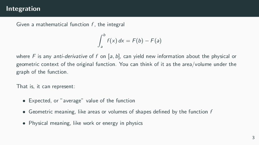
a f (x) dx = F(b) − F(a) where F is any anti-derivative of f on [a, b], can yield new information about the physical or geometric context of the original function. You can think of it as the area/volume under the graph of the function. That is, it can represent: • Expected, or ”average” value of the function • Geometric meaning, like areas or volumes of shapes defined by the function f • Physical meaning, like work or energy in physics 3
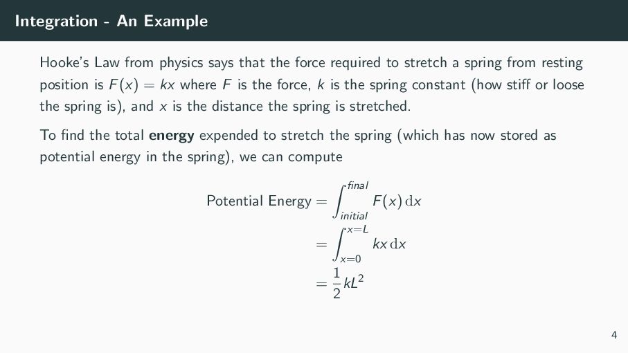
the force required to stretch a spring from resting position is F(x) = kx where F is the force, k is the spring constant (how stiff or loose the spring is), and x is the distance the spring is stretched. To find the total energy expended to stretch the spring (which has now stored as potential energy in the spring), we can compute Potential Energy = final initial F(x) dx = x=L x=0 kx dx = 1 2 kL2 4
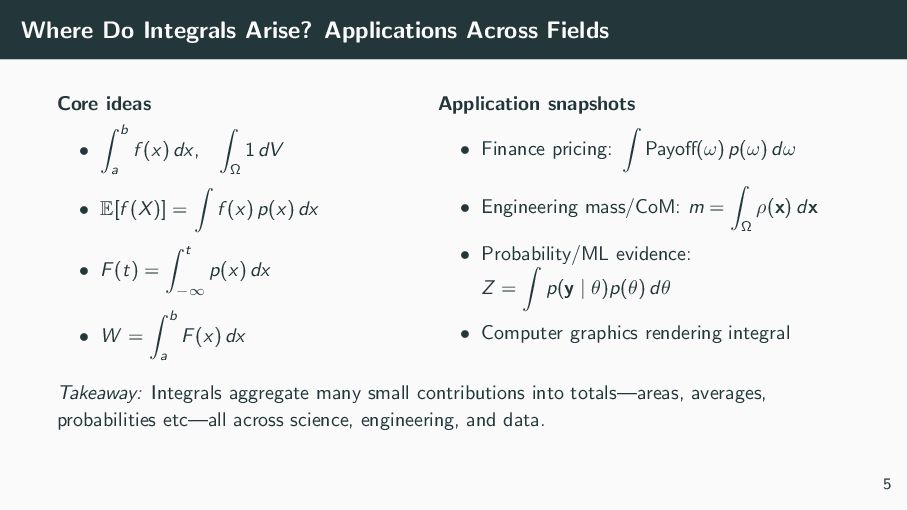
b a f (x) dx, Ω 1 dV • E[f (X)] = f (x) p(x) dx • F(t) = t −∞ p(x) dx • W = b a F(x) dx Application snapshots • Finance pricing: Payoff(ω) p(ω) dω • Engineering mass/CoM: m = Ω ρ(x) dx • Probability/ML evidence: Z = p(y | θ)p(θ) dθ • Computer graphics rendering integral Takeaway: Integrals aggregate many small contributions into totals—areas, averages, probabilities etc—all across science, engineering, and data. 5
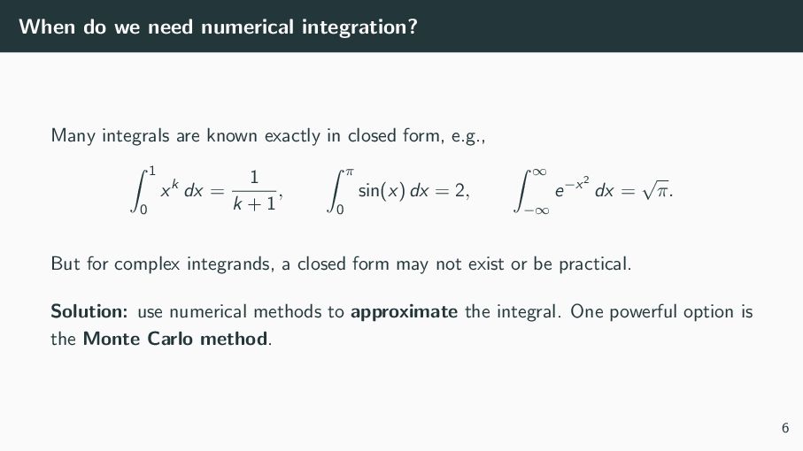
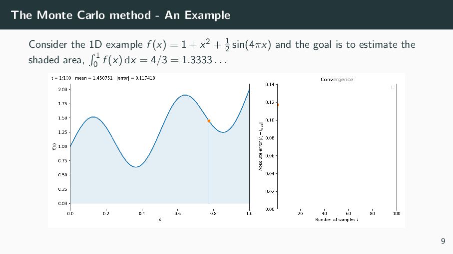
exactly in closed form, e.g., 1 0 xk dx = 1 k + 1 , π 0 sin(x) dx = 2, ∞ −∞ e−x2 dx = √ π. But for complex integrands, a closed form may not exist or be practical. Solution: use numerical methods to approximate the integral. One powerful option is the Monte Carlo method. 6
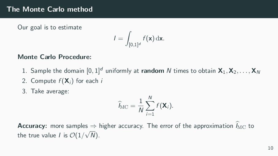
= [0,1]d f (x) dx. Monte Carlo Procedure: 1. Sample the domain [0, 1]d uniformly at random N times to obtain X1, X2, . . . , XN 2. Compute f (Xi ) for each i 3. Take average: IMC = 1 N N i=1 f (Xi ). Accuracy: more samples ⇒ higher accuracy. The error of the approximation IMC to the true value I is O(1/ √ N). 10
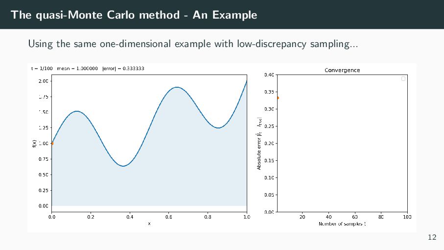
samples by low-discrepancy (LD)–or evenly spread–points X1, . . . , XN ∈ [0, 1]d . 2. Compute f (Xi ) of each i 3. Take average: IQMC = 1 N N i=1 f (Xi ). Accuracy: again, more samples ⇒ higher accuracy, but the error scales now like O(1/N), rather than the slower MC rate of O(1/ √ N). 11
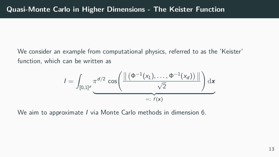
consider an example from computational physics, referred to as the ’Keister’ function, which can be written as I = [0,1]d πd/2 cos Φ−1(x1), . . . , Φ−1(xd ) √ 2 dx =: f (x) We aim to approximate I via Monte Carlo methods in dimension 6. 13
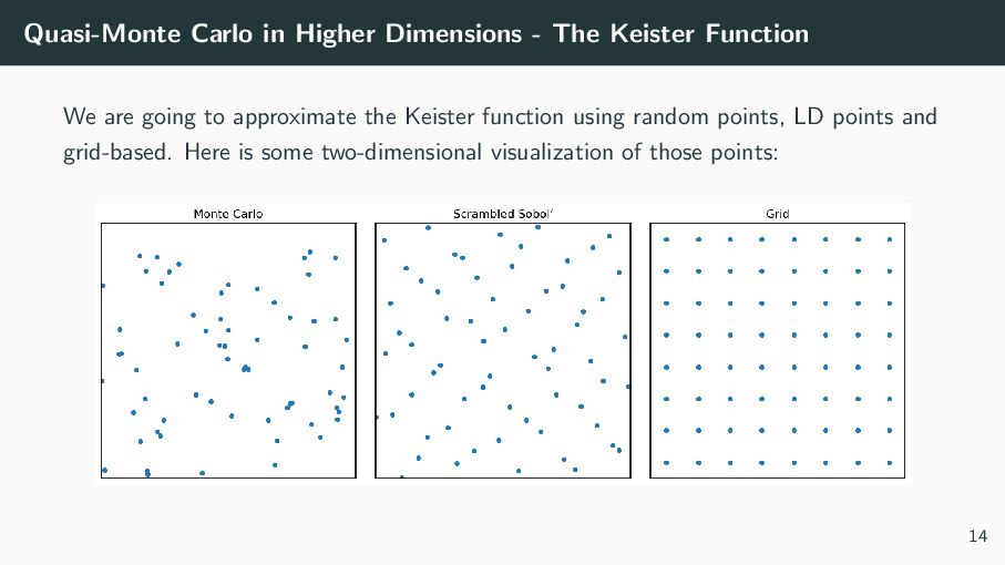
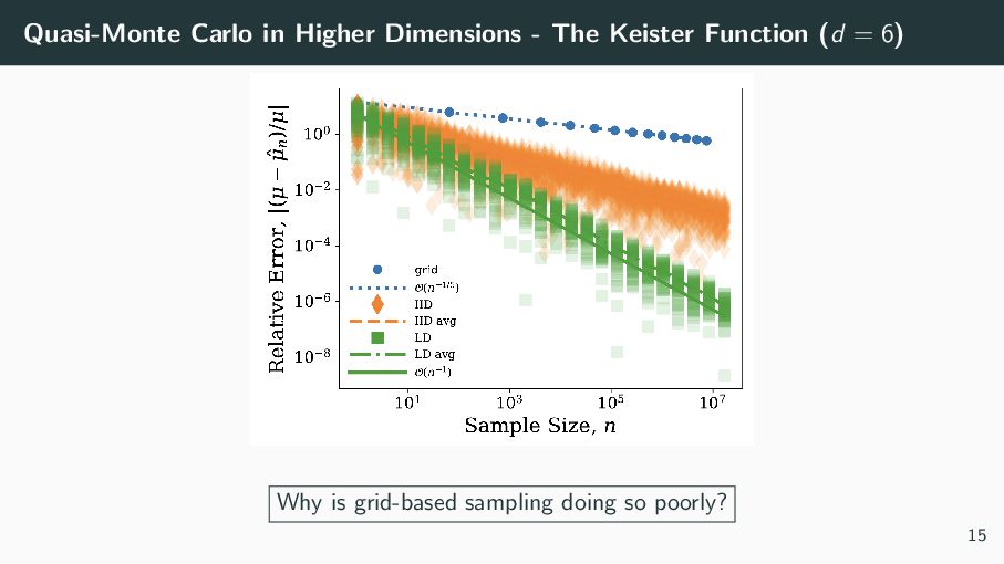
are going to approximate the Keister function using random points, LD points and grid-based. Here is some two-dimensional visualization of those points: 14
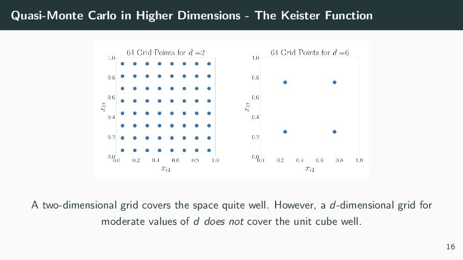
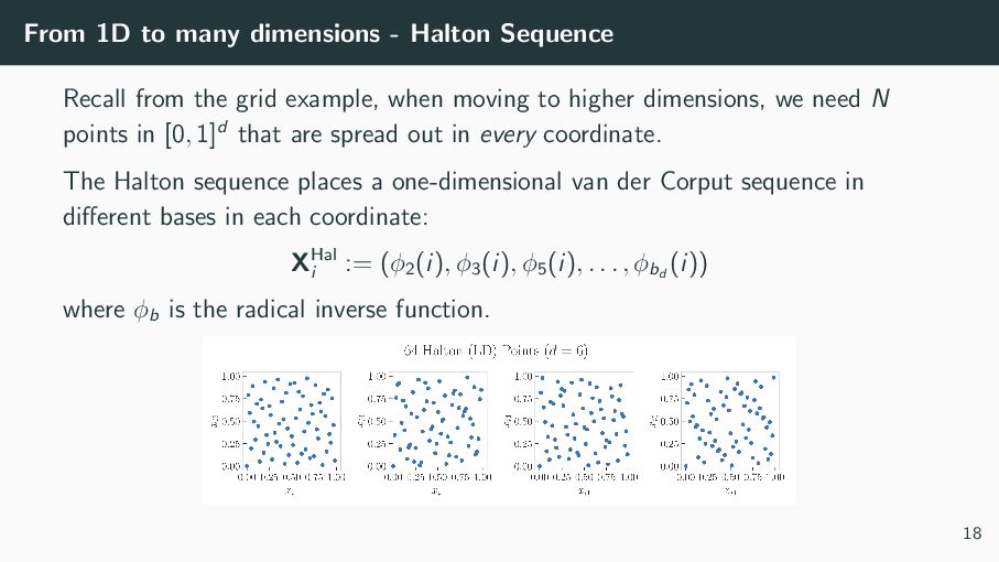
the grid example, when moving to higher dimensions, we need N points in [0, 1]d that are spread out in every coordinate. The Halton sequence places a one-dimensional van der Corput sequence in different bases in each coordinate: XHal i := (ϕ2 (i), ϕ3 (i), ϕ5 (i), . . . , ϕbd (i)) where ϕb is the radical inverse function. 18
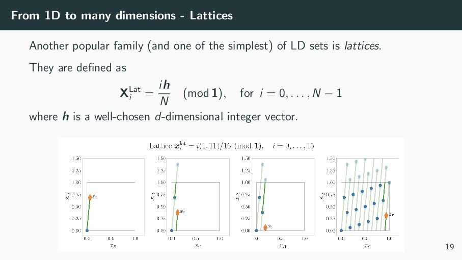
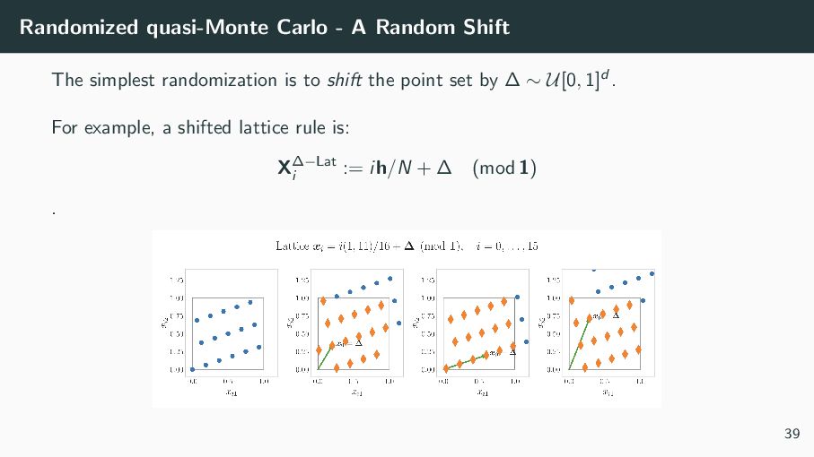
(and one of the simplest) of LD sets is lattices. They are defined as XLat i = ih N (mod 1), for i = 0, . . . , N − 1 where h is a well-chosen d-dimensional integer vector. 19
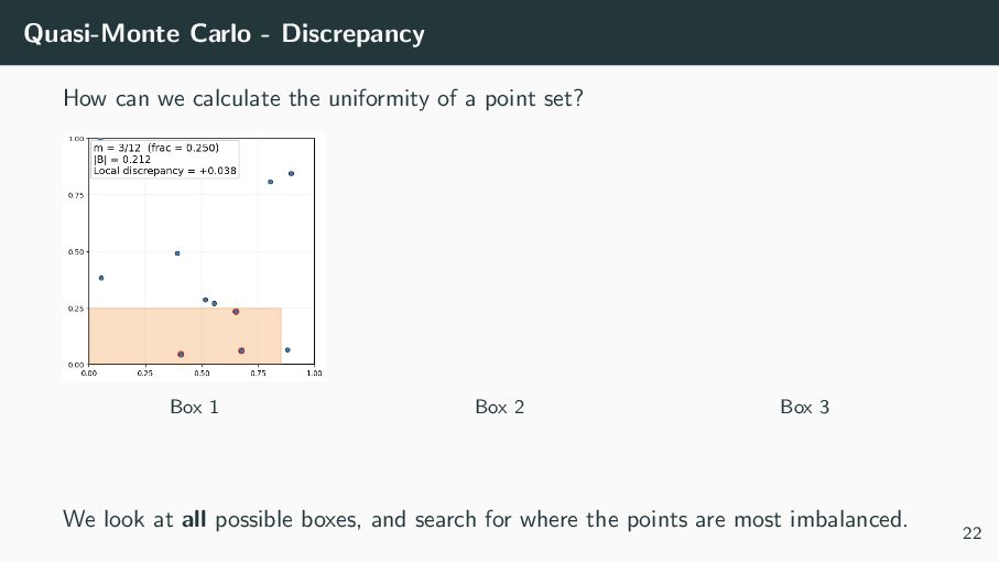
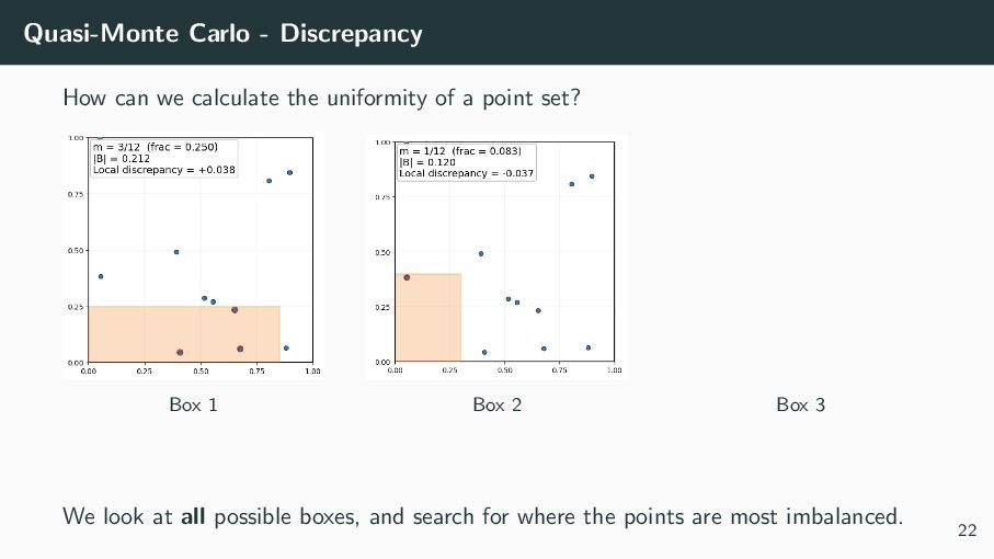
, we can theoretically say that the error of our (Q)MC approximation is at most the product of two terms: 1 N N i=1 f (Xi ) − [0,1]d f (x) dx ≤ V (f ) · D(PN ) where V (f ) is the ”spikeyness” of the function (not in our control), and D(PN ) is the uniformity of the sampling points PN = {X1 , X2 , . . . , XN }, called the discrepancy (our choice!) 21
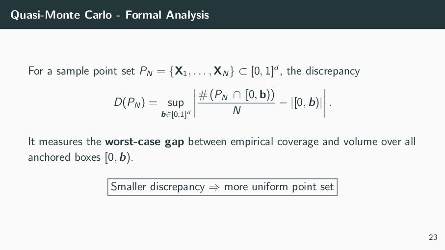
PN = {X1 , . . . , XN } ⊂ [0, 1]d , the discrepancy D(PN ) = sup b∈[0,1]d # (PN ∩ [0, b)) N − |[0, b)| . It measures the worst-case gap between empirical coverage and volume over all anchored boxes [0, b). Smaller discrepancy ⇒ more uniform point set 23
from number theoretic ideas (base 2 expansions, modulo 1 arithmetic, etc...) • analyzed ’asymptotically’, i.e., as N → ∞ or for very very large N Few methods address finding optimal node configurations for specific N and d parameters. Optimizing QMC constructions is what I have contributed to QMC methods 25
an objective function. In our case, we optimize the sampling locations with respect to the discrepancy as the objective function. That is, we solve the following optimization problem: argmin PN ⊂[0,1]d D(PN) 26
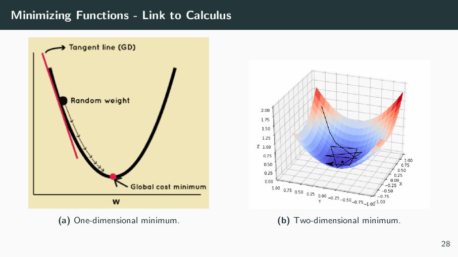
about to know) how to minimize functions! Given a function y = f (x), the optimum (maximum or minimum) will be attained when: dy dx = 0 e.g., for y = (x − 3)3 ⇒ dy dx = 3(x − 3)2 = 0 ⇒ x = 3 attains minimum of y = 0. However, oftentimes, either: • finding the gradient dy/dx is not analytically computable • There may be a few parameter values that all give very similar values (this is called ’local optima’) • Other more complicate reasons why ’first derivaive = 0’ may not work. In this case, you must rely on a numerical method for finding the optimum. 27
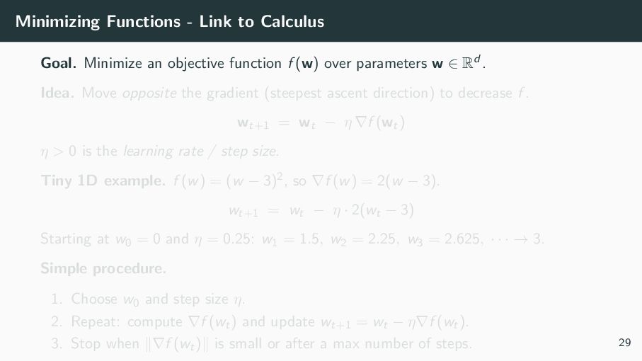
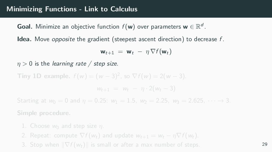
function f (w) over parameters w ∈ Rd . Idea. Move opposite the gradient (steepest ascent direction) to decrease f . wt+1 = wt − η ∇f (wt) η > 0 is the learning rate / step size. Tiny 1D example. f (w) = (w − 3)2, so ∇f (w) = 2(w − 3). wt+1 = wt − η · 2(wt − 3) Starting at w0 = 0 and η = 0.25: w1 = 1.5, w2 = 2.25, w3 = 2.625, · · · → 3. Simple procedure. 1. Choose w0 and step size η. 2. Repeat: compute ∇f (wt) and update wt+1 = wt − η∇f (wt). 3. Stop when ∥∇f (wt)∥ is small or after a max number of steps. 29
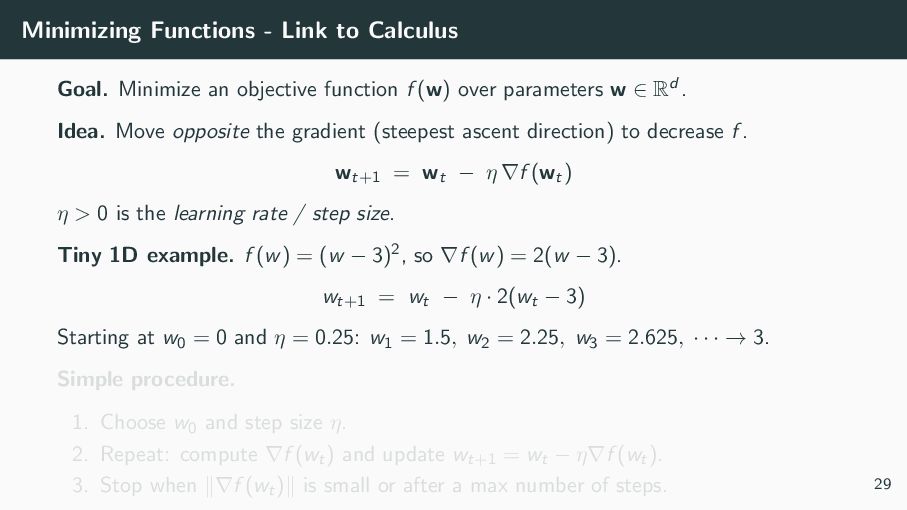
function f (w) over parameters w ∈ Rd . Idea. Move opposite the gradient (steepest ascent direction) to decrease f . wt+1 = wt − η ∇f (wt) η > 0 is the learning rate / step size. Tiny 1D example. f (w) = (w − 3)2, so ∇f (w) = 2(w − 3). wt+1 = wt − η · 2(wt − 3) Starting at w0 = 0 and η = 0.25: w1 = 1.5, w2 = 2.25, w3 = 2.625, · · · → 3. Simple procedure. 1. Choose w0 and step size η. 2. Repeat: compute ∇f (wt) and update wt+1 = wt − η∇f (wt). 3. Stop when ∥∇f (wt)∥ is small or after a max number of steps. 29
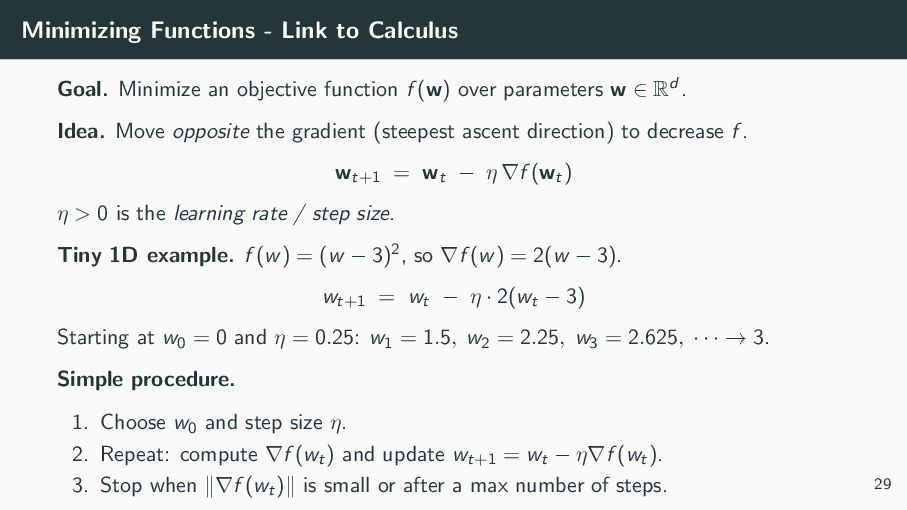
function f (w) over parameters w ∈ Rd . Idea. Move opposite the gradient (steepest ascent direction) to decrease f . wt+1 = wt − η ∇f (wt) η > 0 is the learning rate / step size. Tiny 1D example. f (w) = (w − 3)2, so ∇f (w) = 2(w − 3). wt+1 = wt − η · 2(wt − 3) Starting at w0 = 0 and η = 0.25: w1 = 1.5, w2 = 2.25, w3 = 2.625, · · · → 3. Simple procedure. 1. Choose w0 and step size η. 2. Repeat: compute ∇f (wt) and update wt+1 = wt − η∇f (wt). 3. Stop when ∥∇f (wt)∥ is small or after a max number of steps. 29
function f (w) over parameters w ∈ Rd . Idea. Move opposite the gradient (steepest ascent direction) to decrease f . wt+1 = wt − η ∇f (wt) η > 0 is the learning rate / step size. Tiny 1D example. f (w) = (w − 3)2, so ∇f (w) = 2(w − 3). wt+1 = wt − η · 2(wt − 3) Starting at w0 = 0 and η = 0.25: w1 = 1.5, w2 = 2.25, w3 = 2.625, · · · → 3. Simple procedure. 1. Choose w0 and step size η. 2. Repeat: compute ∇f (wt) and update wt+1 = wt − η∇f (wt). 3. Stop when ∥∇f (wt)∥ is small or after a max number of steps. 29
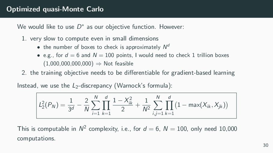
our objective function. However: 1. very slow to compute even in small dimensions • the number of boxes to check is approximately Nd • e.g., for d = 6 and N = 100 points, I would need to check 1 trillion boxes (1,000,000,000,000) ⇒ Not feasible 2. the training objective needs to be differentiable for gradient-based learning Instead, we use the L2-discrepancy (Warnock’s formula): L2 2 (PN) = 1 3d − 2 N N i=1 d k=1 1 − X2 ik 2 + 1 N2 N i,j=1 d k=1 1 − max(Xik, Xjk) This is computable in N2 complexity, i.e., for d = 6, N = 100, only need 10,000 computations. 30
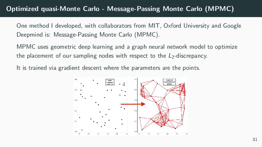
I developed, with collaborators from MIT, Oxford University and Google Deepmind is: Message-Passing Monte Carlo (MPMC). MPMC uses geometric deep learning and a graph neural network model to optimize the placement of our sampling nodes with respect to the L2-discrepancy. It is trained via gradient descent where the parameters are the points. 31
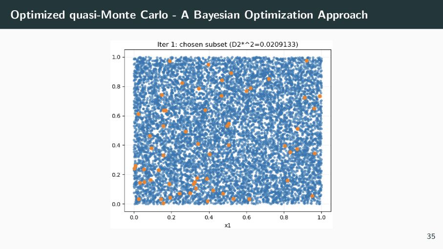
approach I am currently developing with an Illinois Tech Masters student is a Subset Selection problem. We now start with a large N population set PN, and attempt to choose the best m < N points to minimize the discrepancy. That is, we wish to solve argmin Pm⊂PN , m<N D(Pm) We cannot check all subsets one-by-one. There are N m many. e.g, to find the ’best’ m = 50 points from N = 1000, we would need to check 946046101758521784606372227772804491872969400166865406479356932134325269719811 possible combinations! 33
a Bayesian Optimization (BO) strategy to solve the subset selection problem. It does not use gradient descent. Instead, relies on probabilistic modeling. BO is an optimization strategy that predicts the value, and gives uncertainty (error) its prediction. It uses this information to intelligently choose where to sample next. It efficiently balances exploration of unknown regions and exploitation of promising areas to find the optimum in as few evaluations as possible. 34
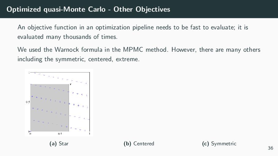
an optimization pipeline needs to be fast to evaluate; it is evaluated many thousands of times. We used the Warnock formula in the MPMC method. However, there are many others including the symmetric, centered, extreme. (a) Star (b) Centered (c) Symmetric 36
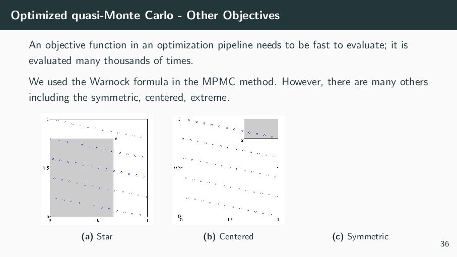
an optimization pipeline needs to be fast to evaluate; it is evaluated many thousands of times. We used the Warnock formula in the MPMC method. However, there are many others including the symmetric, centered, extreme. (a) Star (b) Centered (c) Symmetric 36
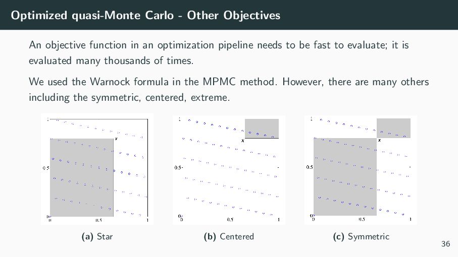
an optimization pipeline needs to be fast to evaluate; it is evaluated many thousands of times. We used the Warnock formula in the MPMC method. However, there are many others including the symmetric, centered, extreme. (a) Star (b) Centered (c) Symmetric 36
sample mean I does not change across runs, like IID nodes would. While determinism has advantages, randomization has substantial advantages as well: • Randomization (done correctly) removes bias from the estimator • Replications can facilitate error estimates (think: confidence intervals) A good randomization must preserve the LD property of the QMC construction. 38
G. Sorokin, Quasi-Monte Carlo Methods: What, Why and How?, Proc. MCQMC 2024. Available at: https://arxiv.org/abs/2502.03644 • J. Dick and F. Pillichshammer, Digital Nets and Sequences, Cambridge, 2010. • A. B. Owen, Monte Carlo Theory, Methods and Examples, 2013–, online book. https://artowen.su.domains/mc/ 41