Aggregate Demand And Supply

Transcript

1. AGGREGATE SUPPLY AND AGGREGATE DEMAND
2. Objectives After studying this chapter, you will able to  Explain what determines aggregate supply  Explain what determines aggregate demand  Explain macroeconomic equilibrium  Explain the effects of changes in aggregate supply and aggregate demand on economic growth, inflation, and business cycles  Explain economic growth, inflation, and business cycles by using the AS-AD model
3. Production and Prices What forces bring persistent and rapid expansion of real GDP? What causes inflation? Why do we have business cycles? How do policy actions by the government and the Federal Reserve affect output and prices?
4. Aggregate Supply Aggregate Supply Fundamentals The aggregate quantity of goods and services supplied depends on three factors:  The quantity of labor (L )  The quantity of capital (K )  The state of technology (T ) The aggregate production function shows how quantity of real GDP supplied, Y, depends on labor, capital, and technology.
5. Aggregate Supply The aggregate production function is written as the equation: Y = F(L, K, T ). In words, the quantity of real GDP supplied depends on (is a function of) the quantity of labor employed, the quantity of capital, and the state of technology. The larger is L, K, or T, the greater is Y.
6. Aggregate Supply At any given time, the quantity of capital and the state of technology are fixed but the quantity of labor can vary. The higher the real wage rate, the smaller is the quantity of labor demanded and the greater is the quantity of labor supplied. The wage rate that makes the quantity of labor demanded equal to the quantity supplied is the equilibrium wage rate and at that wage the level of employment is the natural rate of unemployment.
7. Aggregate Supply We distinguish two time frames associated with different states of the labor market:  Long-run aggregate supply  Short-run aggregate supply
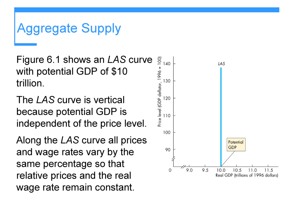
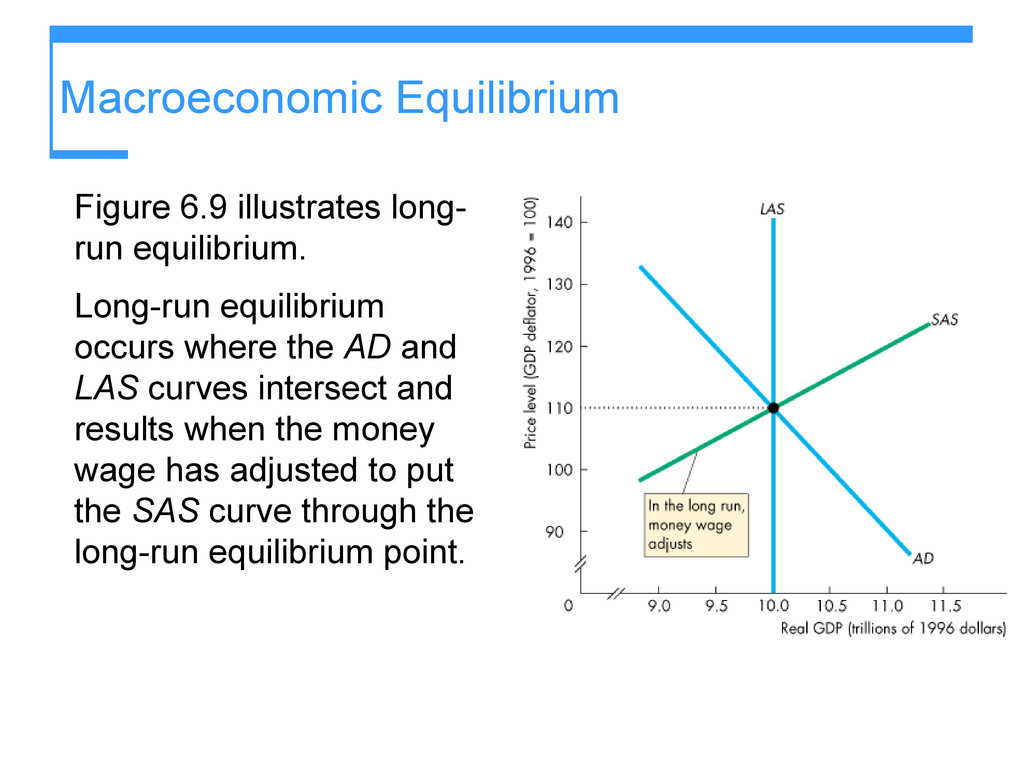
8. Aggregate Supply Long-Run Aggregate Supply The macroeconomic long run is a time frame that is sufficiently long for all adjustments to be made so that real GDP equals potential GDP and there is full employment. The long-run aggregate supply curve (LAS) is the relationship between the quantity of real GDP supplied and the price level when real GDP equals potential GDP.
9. Aggregate Supply Figure 6.1 shows an LAS curve with potential GDP of $10 trillion. The LAS curve is vertical because potential GDP is independent of the price level. Along the LAS curve all prices and wage rates vary by the same percentage so that relative prices and the real wage rate remain constant.
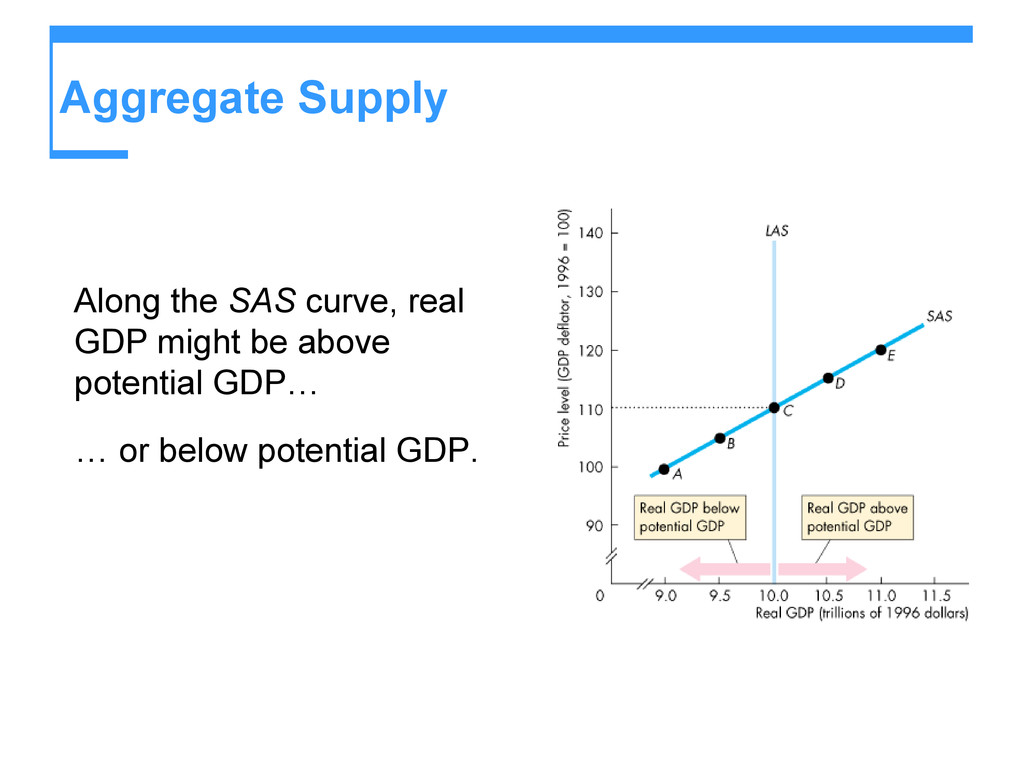
10. Aggregate Supply Short-Run Aggregate Supply The macroeconomic short run is a period during which real GDP has fallen below or risen above potential GDP. At the same time, the unemployment rate has risen above or fallen below the natural unemployment rate. The short-run aggregate supply curve (SAS) is the relationship between the quantity of real GDP supplied and the price level in the short run when the money wage rate, the prices of other resources, and potential GDP remain constant.
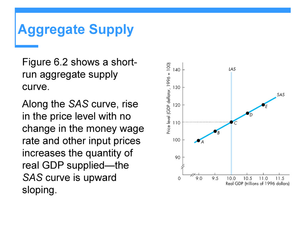
11. Aggregate Supply Figure 6.2 shows a short- run aggregate supply curve. Along the SAS curve, rise in the price level with no change in the money wage rate and other input prices increases the quantity of real GDP supplied—the SAS curve is upward sloping.
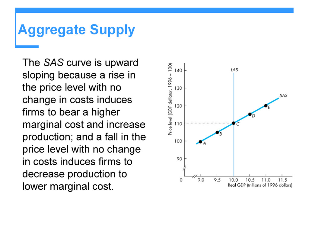
12. Aggregate Supply The SAS curve is upward sloping because a rise in the price level with no change in costs induces firms to bear a higher marginal cost and increase production; and a fall in the price level with no change in costs induces firms to decrease production to lower marginal cost.
13. Aggregate Supply Along the SAS curve, real GDP might be above potential GDP… … or below potential GDP.
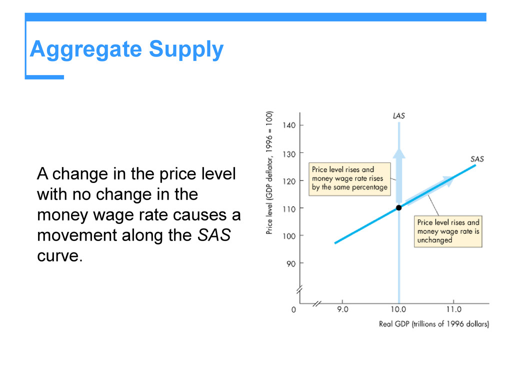
14. Aggregate Supply Movement along the LAS and SAS Curves Figure 6.3 summarizes what you’ve just learned about the LAS and SAS curves. A change in the price level with an equal percentage change in the money wage rate causes a movement along the LAS curve.
15. Aggregate Supply A change in the price level with no change in the money wage rate causes a movement along the SAS curve.
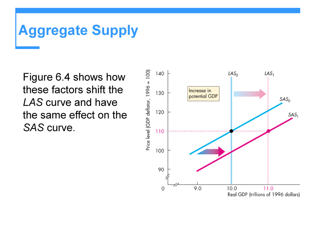
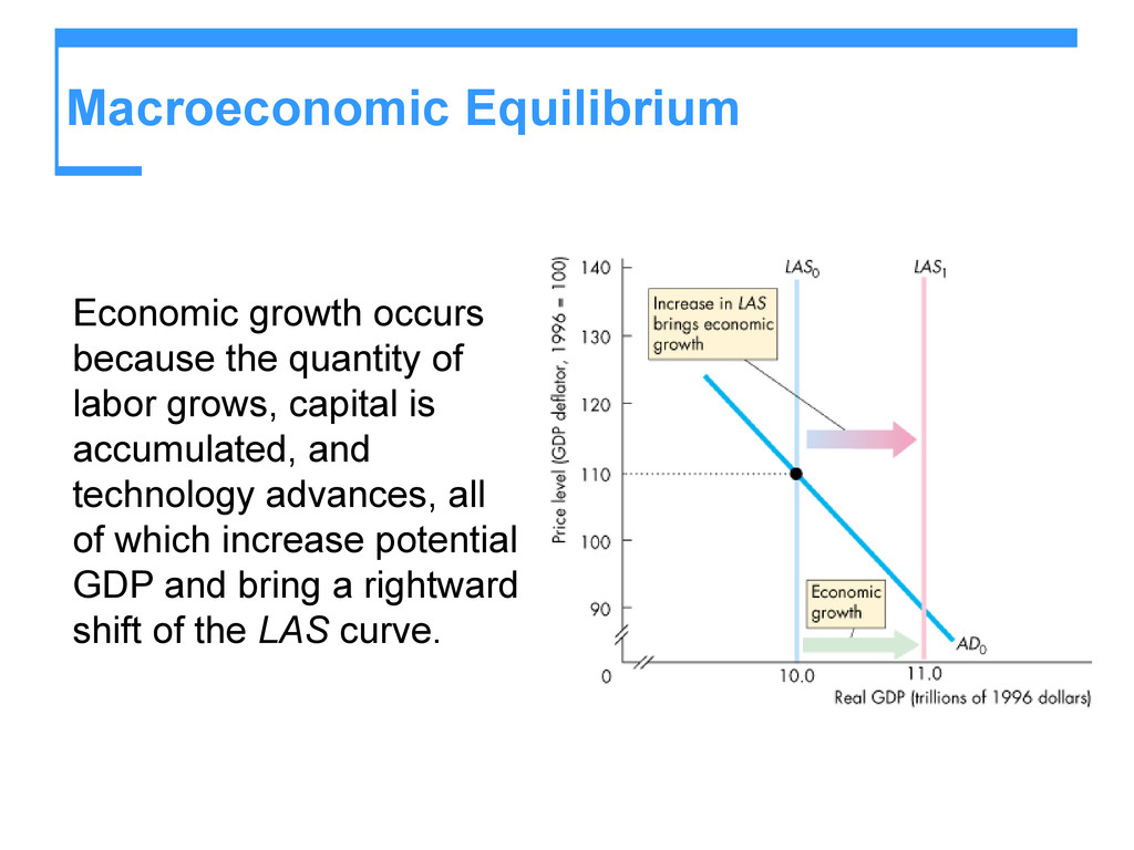
16. Aggregate Supply Changes in Aggregate Supply When potential GDP increases, both the LAS and SAS curves shift rightward. Potential GDP changes, for three reasons:  Change in the full-employment quantity of labor  Change in the quantity of capital (physical or human)  Advance in technology
17. Aggregate Supply Figure 6.4 shows how these factors shift the LAS curve and have the same effect on the SAS curve.
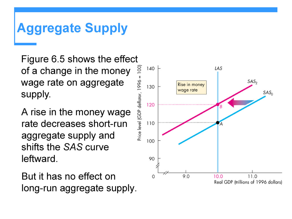
18. Aggregate Supply Figure 6.5 shows the effect of a change in the money wage rate on aggregate supply. A rise in the money wage rate decreases short-run aggregate supply and shifts the SAS curve leftward. But it has no effect on long-run aggregate supply.
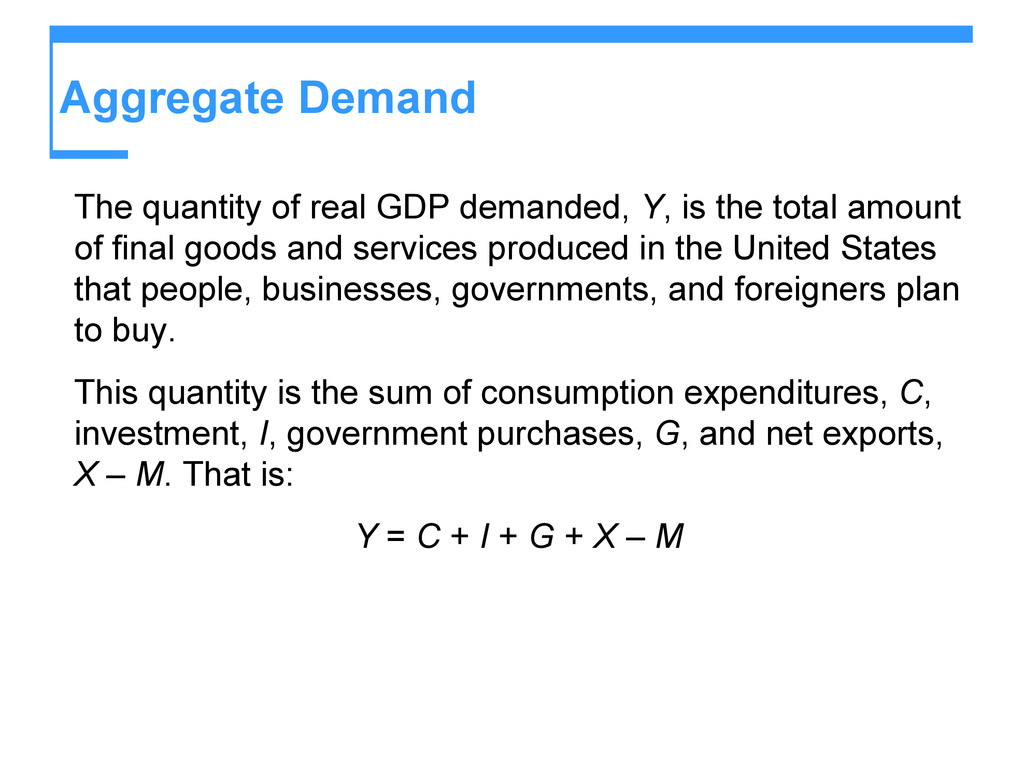
19. Aggregate Demand The quantity of real GDP demanded, Y, is the total amount of final goods and services produced in the United States that people, businesses, governments, and foreigners plan to buy. This quantity is the sum of consumption expenditures, C, investment, I, government purchases, G, and net exports, X – M. That is: Y = C + I + G + X – M
20. Aggregate Demand Buying plans depend on many factors and some of the main ones are:  The price level  Expectations  Fiscal and monetary policy  The world economy
21. Aggregate Demand The Aggregate Demand Curve Aggregate demand is the relationship between the quantity of real GDP demanded and the price level. The aggregate demand (AD) curve plots the quantity of real GDP demanded against the price level.
22. Aggregate Demand Figure 6.6 shows an AD curve. The AD curve slopes downward for two reasons:  A wealth effect  Substitution effects
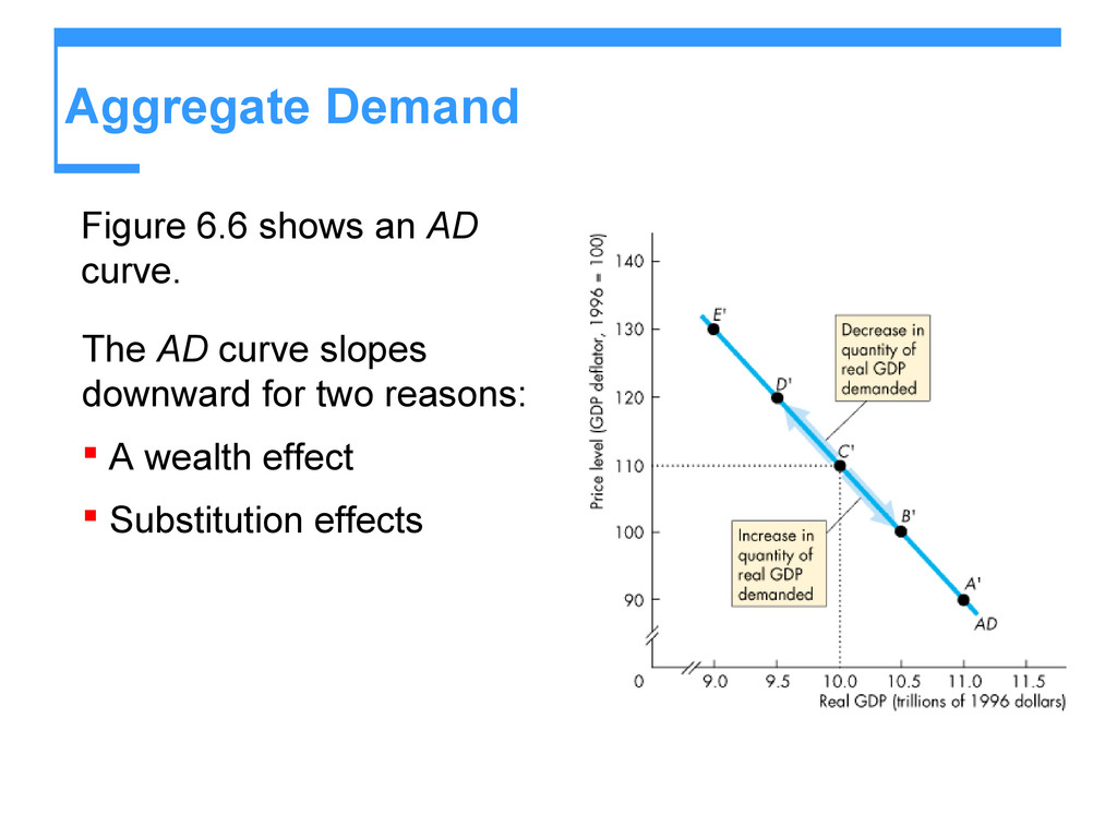
23. Aggregate Demand Wealth effect A rise in the price level, other things remaining the same, decreases the quantity of real wealth (money, bonds, stocks, etc.). To restore their real wealth, people increase saving and decrease spending, so the quantity of real GDP demanded decreases. Similarly, a fall in the price level, other things remaining the same, increases the quantity of real wealth. With more real wealth, people decrease saving and increase spending, so the quantity of real GDP demanded increases.
24. Aggregate Demand Intertemporal substitution effect A rise in the price level, other things remaining the same, decreases the real value of money and raises the interest rate. Faced with a higher interest rate, people try to borrow and spend less so the quantity of real GDP demanded decreases. Similarly, a fall in the price level increases the real value of money and lowers the interest rate. Faced with a lower interest rate, people borrow and spend more so the quantity of real GDP demanded increases.
25. Aggregate Demand International substitution effect A rise in the price level, other things remaining the same, increases the price of domestic goods relative to foreign goods, so imports increase and exports decrease, which decreases the quantity of real GDP demanded. Similarly, a fall in the price level, other things remaining the same, decreases the price of domestic goods relative to foreign goods, so imports decrease and exports increase, which increases the quantity of real GDP demanded.
26. Aggregate Demand Changes in Aggregate Demand A change in any influence on buying plans other than the price level changes aggregate demand. The main influences on aggregate demand are:  Expectations  Fiscal and monetary policy  The world economy
27. Aggregate Demand Expectations about future income, future inflation, and future profits change aggregate demand. Increases in expected future income increase people’s consumption today, and increases aggregate demand. A rise in the expected inflation rate makes buying goods cheaper today and increases aggregate demand. An increase in expected future profits boosts firms’ investment, which increases aggregate demand.
28. Aggregate Demand Fiscal policy is the government’s attempt to influence economic activity by changing its taxes, spending, deficit, and debt policies. A tax cut or an increase in transfer payments increases households’ disposable income—aggregate income minus taxes plus transfer payments. An increase in disposable income increases consumption expenditure and increases aggregate demand.
29. Aggregate Demand Because government purchases of goods and services are one component of aggregate demand, an increase in government purchases increases aggregate demand. Monetary policy is changes in the interest rate and quantity of money. An increase in the quantity of money increases buying power and increases aggregate demand. A cut in the interest rate increases expenditure and increases aggregate demand.
30. Aggregate Demand The world economy influences aggregate demand in two ways: A fall in the foreign exchange rate lowers the price of domestic goods and services relative to foreign goods and services, increases exports, decreases imports, and increases aggregate demand. An increase in foreign income increases the demand for U.S. exports and increases aggregate demand.
31. Aggregate Demand Figure 6.7 illustrates changes in aggregate demand. When aggregate demand increases, the AD curve shifts rightward… … and when aggregate demand decreases, the AD curve shifts leftward.
32. Macroeconomic Equilibrium Short-Run Macroeconomic Equilibrium Short-run macroeconomic equilibrium occurs when the quantity of real GDP demanded equals the quantity of real GDP supplied at the point of intersection of the AD curve and the SAS curve.
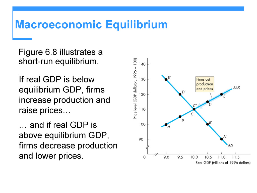
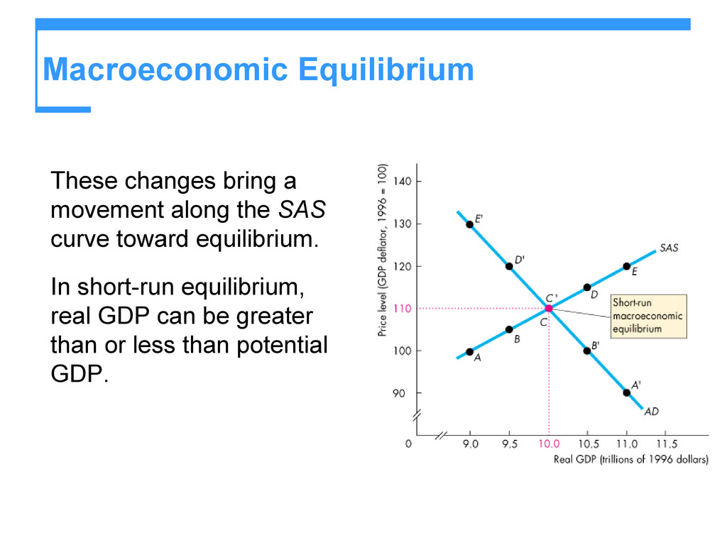
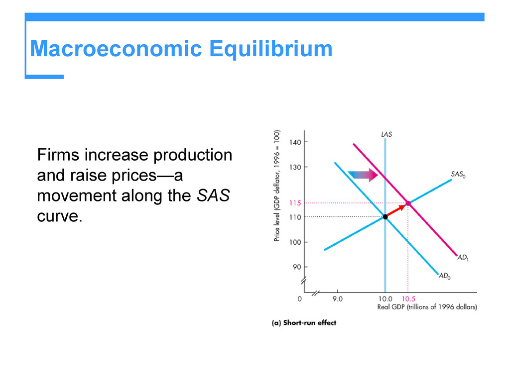
33. Macroeconomic Equilibrium Figure 6.8 illustrates a short-run equilibrium. If real GDP is below equilibrium GDP, firms increase production and raise prices… … and if real GDP is above equilibrium GDP, firms decrease production and lower prices.
34. Macroeconomic Equilibrium These changes bring a movement along the SAS curve toward equilibrium. In short-run equilibrium, real GDP can be greater than or less than potential GDP.
35. Macroeconomic Equilibrium Long-Run Macroeconomic Equilibrium Long-run macroeconomic equilibrium occurs when real GDP equals potential GDP—when the economy is on its LAS curve.
36. Macroeconomic Equilibrium Figure 6.9 illustrates long- run equilibrium. Long-run equilibrium occurs where the AD and LAS curves intersect and results when the money wage has adjusted to put the SAS curve through the long-run equilibrium point.
37. Macroeconomic Equilibrium Economic Growth and Inflation Figure 6.10 illustrates economic growth and inflation.
38. Macroeconomic Equilibrium Economic growth occurs because the quantity of labor grows, capital is accumulated, and technology advances, all of which increase potential GDP and bring a rightward shift of the LAS curve.
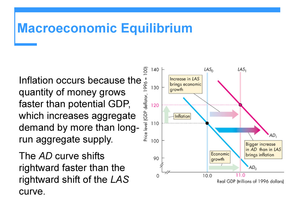
39. Macroeconomic Equilibrium Inflation occurs because the quantity of money grows faster than potential GDP, which increases aggregate demand by more than long- run aggregate supply. The AD curve shifts rightward faster than the rightward shift of the LAS curve.
40. Macroeconomic Equilibrium The Business Cycle The business cycle occurs because aggregate demand and the short-run aggregate supply fluctuate but the money wage rate does not change rapidly enough to keep real GDP at potential GDP.
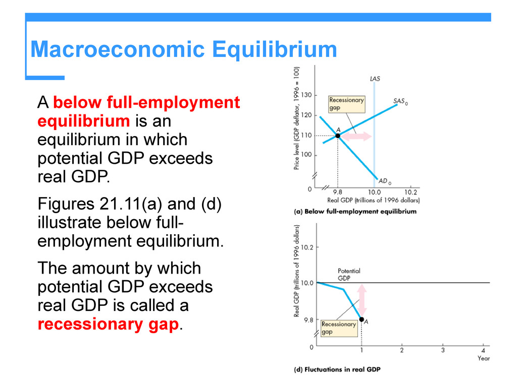
41. Macroeconomic Equilibrium A below full-employment equilibrium is an equilibrium in which potential GDP exceeds real GDP. Figures 21.11(a) and (d) illustrate below full- employment equilibrium. The amount by which potential GDP exceeds real GDP is called a recessionary gap.
42. Macroeconomic Equilibrium A long-run equilibrium is an equilibrium in which potential GDP equals real GDP. Figures 21.11(b) and (d) illustrate long-run equilibrium.
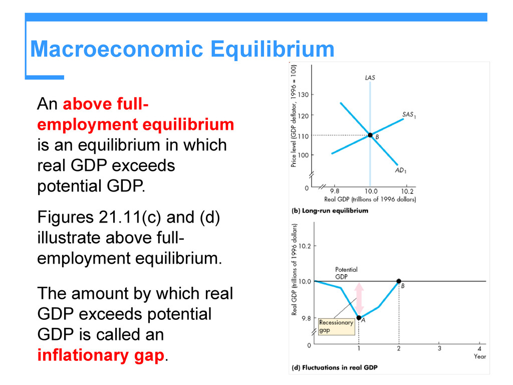
43. Macroeconomic Equilibrium An above full- employment equilibrium is an equilibrium in which real GDP exceeds potential GDP. Figures 21.11(c) and (d) illustrate above full- employment equilibrium. The amount by which real GDP exceeds potential GDP is called an inflationary gap.
44. Macroeconomic Equilibrium Figure 6.11(d) shows how, as the economy moves from one type of short-run equilibrium to another, real GDP fluctuates around potential GDP in a business cycle.
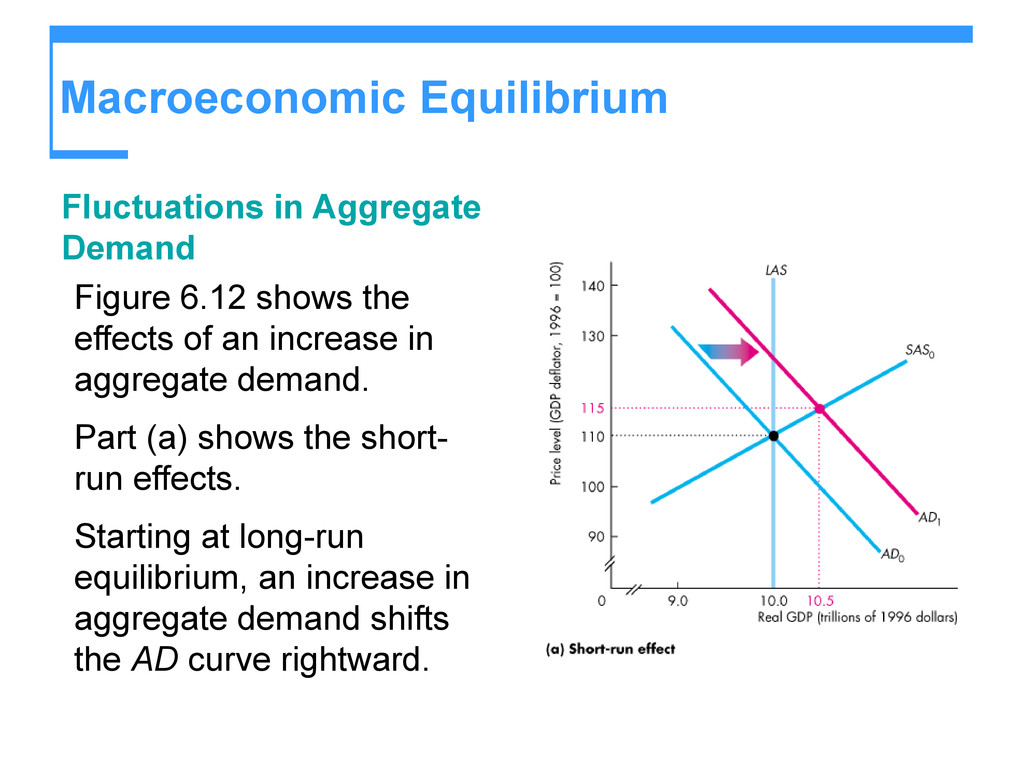
45. Macroeconomic Equilibrium Fluctuations in Aggregate Demand Figure 6.12 shows the effects of an increase in aggregate demand. Part (a) shows the short- run effects. Starting at long-run equilibrium, an increase in aggregate demand shifts the AD curve rightward.
46. Macroeconomic Equilibrium Firms increase production and raise prices—a movement along the SAS curve.
47. Macroeconomic Equilibrium Figure 6.12(b) shows the long-run effects. Real GDP increases, the price level rises, and in the new short-run equilibrium, there is an inflationary gap.
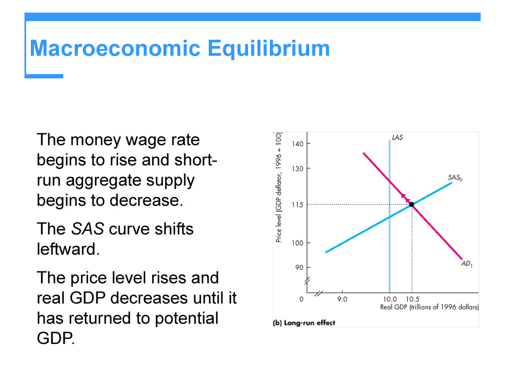
48. Macroeconomic Equilibrium The money wage rate begins to rise and short- run aggregate supply begins to decrease. The SAS curve shifts leftward. The price level rises and real GDP decreases until it has returned to potential GDP.
49. Macroeconomic Equilibrium Fluctuations in Aggregate Supply Figure 6.13 shows the effects of a decrease in aggregate supply. Starting at long-run equilibrium, a rise in the price of oil decreases short-run aggregate supply and the SAS curve shifts leftward.
50. Macroeconomic Equilibrium Real GDP decreases and the price level rises. The combination of recession combined with inflation is called stagflation.
51. U.S. Economic Growth, Inflation, and Cycles Figure 6.14 interprets the changes in real GDP and the price level each year from 1960 to 2001 in terms of shifting AD, SAS, and LAS curves.
52. U.S. Economic Growth, Inflation, and Cycles The figure shows the business cycle, …inflation,… …and long-term economic growth.
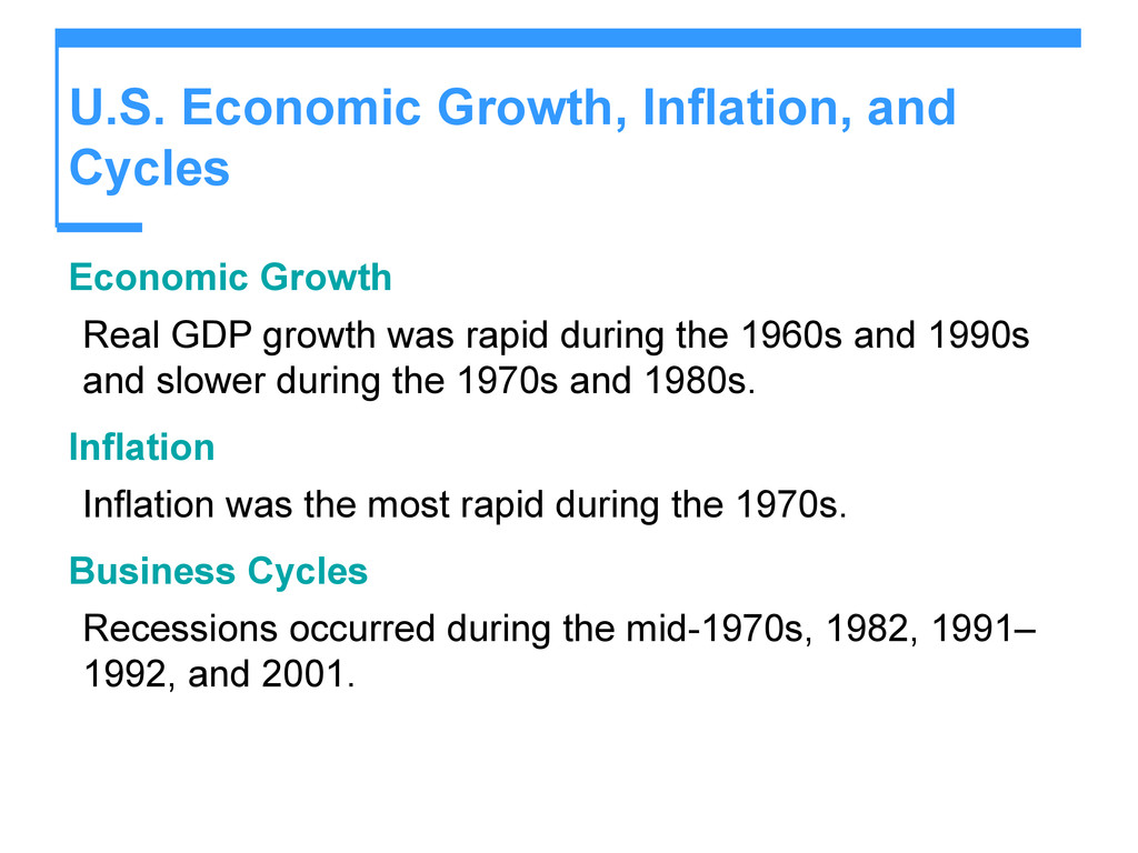
53. Example:U.S. Economic Growth, Inflation, and Cycles From1960 to 2001: Real GDP and potential GDP grew from $2.4 trillion to $9.3 trillion. The price level rose from 22 to 109. Business cycle expansions alternated with recessions.
54. U.S. Economic Growth, Inflation, and Cycles Economic Growth Real GDP growth was rapid during the 1960s and 1990s and slower during the 1970s and 1980s. Inflation Inflation was the most rapid during the 1970s. Business Cycles Recessions occurred during the mid-1970s, 1982, 1991– 1992, and 2001.
55. THE END AGGREGATE SUPPLY AND AGGREGATE DEMAND