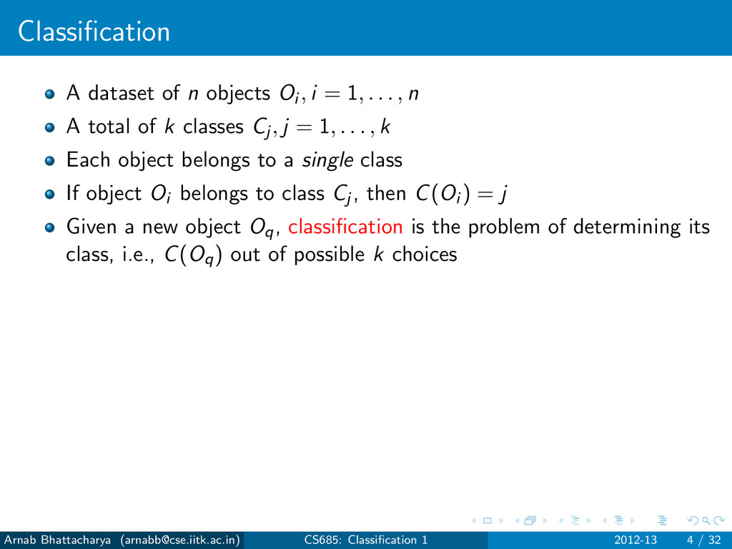
1, . . . , n A total of k classes Cj , j = 1, . . . , k Each object belongs to a single class If object Oi belongs to class Cj , then C(Oi ) = j Given a new object Oq, classification is the problem of determining its class, i.e., C(Oq) out of possible k choices Arnab Bhattacharya ([email protected]) CS685: Classification 1 2012-13 4 / 32
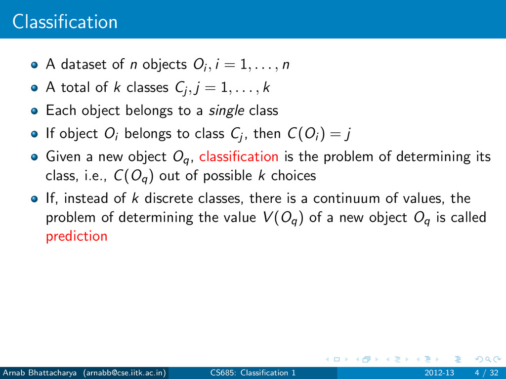
1, . . . , n A total of k classes Cj , j = 1, . . . , k Each object belongs to a single class If object Oi belongs to class Cj , then C(Oi ) = j Given a new object Oq, classification is the problem of determining its class, i.e., C(Oq) out of possible k choices If, instead of k discrete classes, there is a continuum of values, the problem of determining the value V (Oq) of a new object Oq is called prediction Arnab Bhattacharya ([email protected]) CS685: Classification 1 2012-13 4 / 32
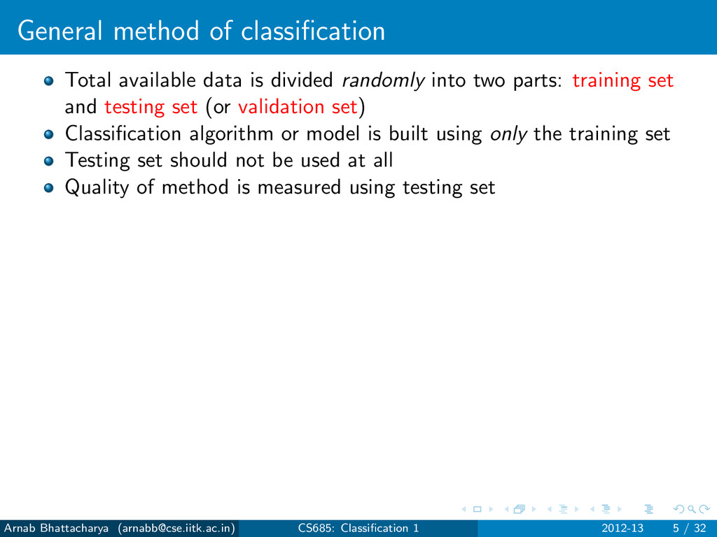
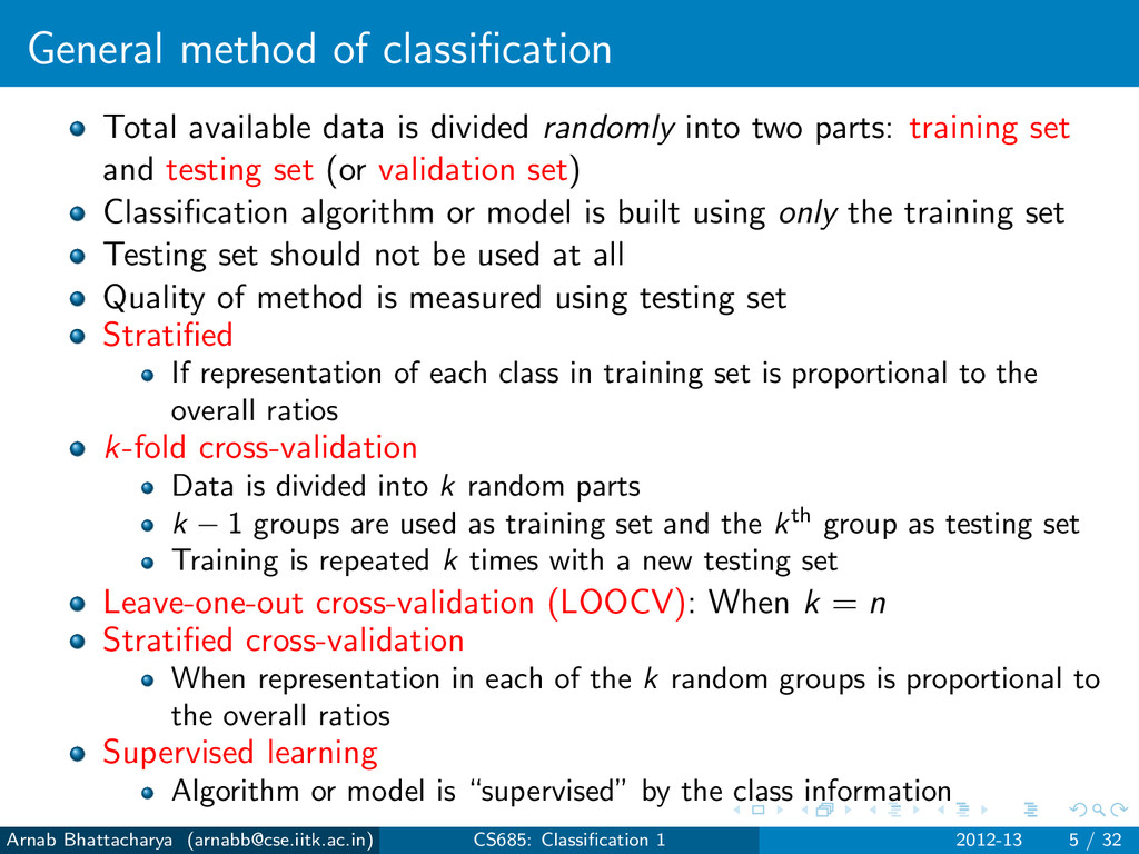
into two parts: training set and testing set (or validation set) Classification algorithm or model is built using only the training set Testing set should not be used at all Quality of method is measured using testing set Arnab Bhattacharya ([email protected]) CS685: Classification 1 2012-13 5 / 32
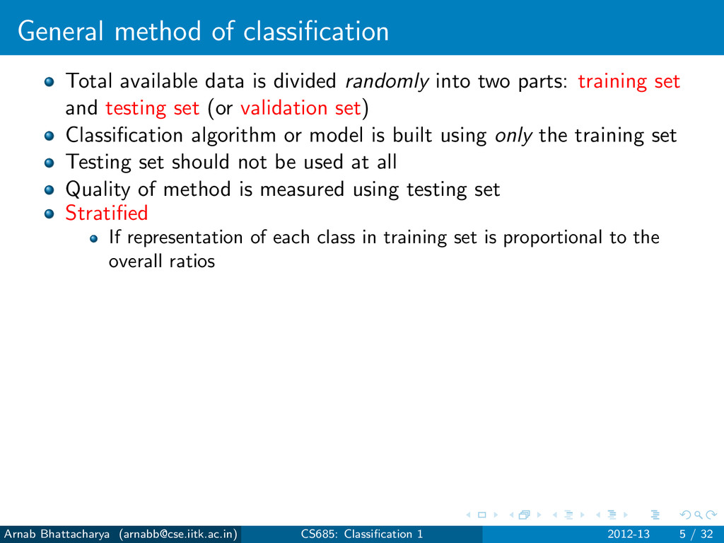
into two parts: training set and testing set (or validation set) Classification algorithm or model is built using only the training set Testing set should not be used at all Quality of method is measured using testing set Stratified If representation of each class in training set is proportional to the overall ratios Arnab Bhattacharya ([email protected]) CS685: Classification 1 2012-13 5 / 32
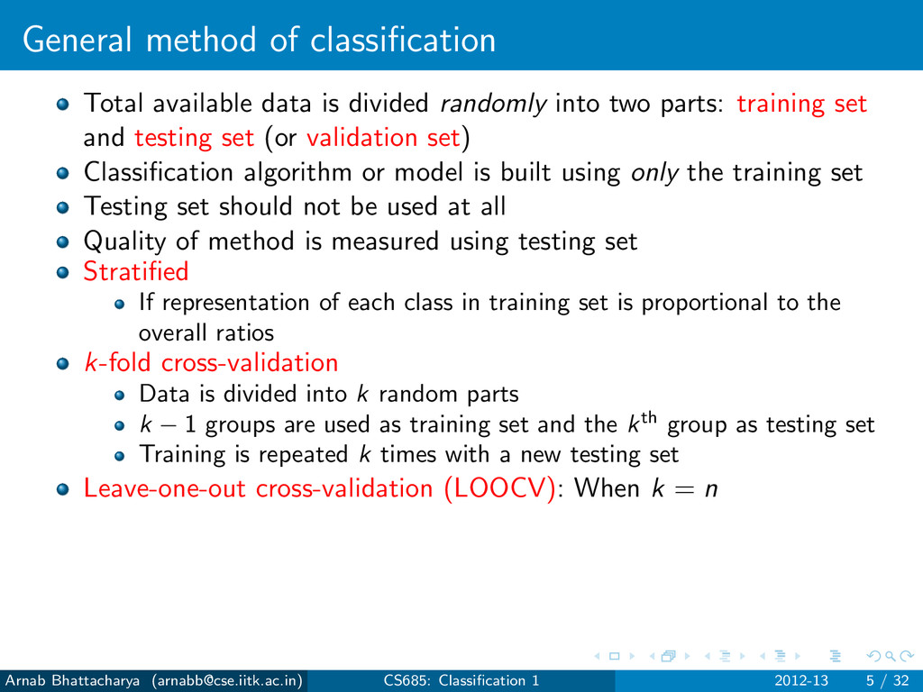
into two parts: training set and testing set (or validation set) Classification algorithm or model is built using only the training set Testing set should not be used at all Quality of method is measured using testing set Stratified If representation of each class in training set is proportional to the overall ratios k-fold cross-validation Data is divided into k random parts k − 1 groups are used as training set and the kth group as testing set Training is repeated k times with a new testing set Leave-one-out cross-validation (LOOCV): When k = n Arnab Bhattacharya ([email protected]) CS685: Classification 1 2012-13 5 / 32
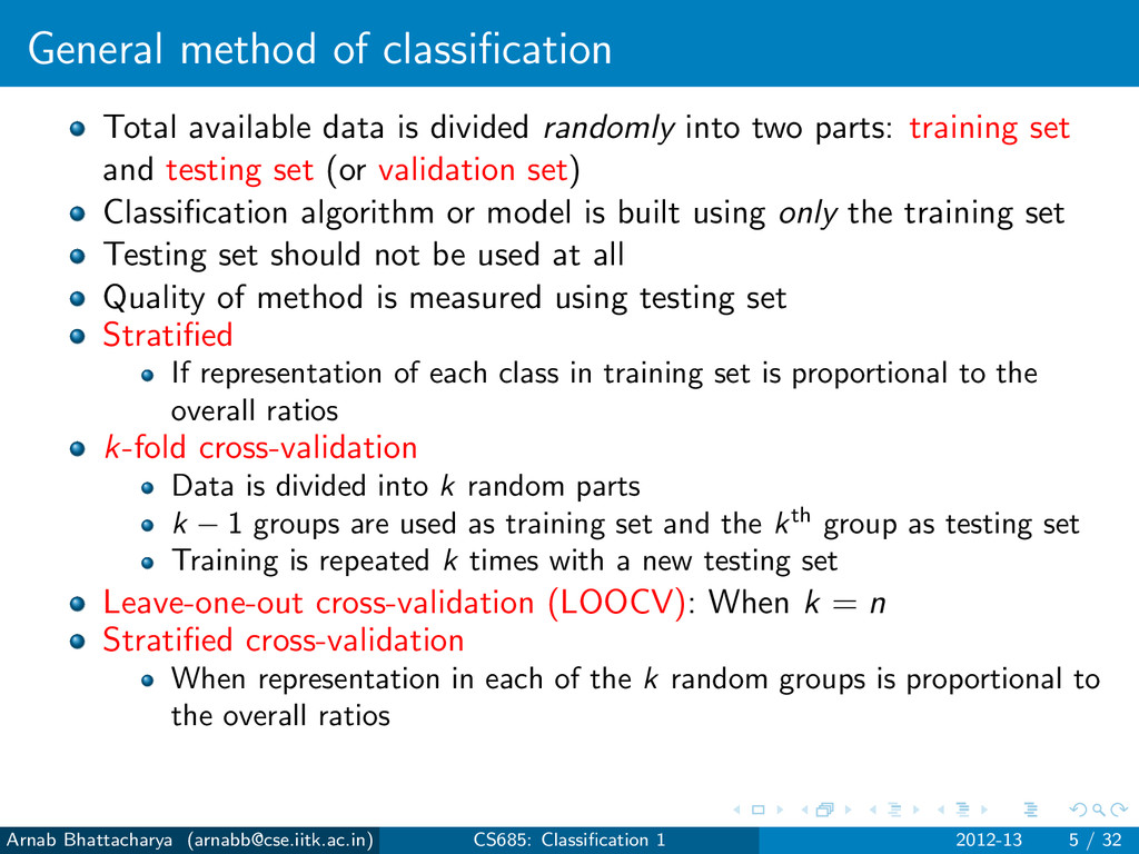
into two parts: training set and testing set (or validation set) Classification algorithm or model is built using only the training set Testing set should not be used at all Quality of method is measured using testing set Stratified If representation of each class in training set is proportional to the overall ratios k-fold cross-validation Data is divided into k random parts k − 1 groups are used as training set and the kth group as testing set Training is repeated k times with a new testing set Leave-one-out cross-validation (LOOCV): When k = n Stratified cross-validation When representation in each of the k random groups is proportional to the overall ratios Arnab Bhattacharya ([email protected]) CS685: Classification 1 2012-13 5 / 32
into two parts: training set and testing set (or validation set) Classification algorithm or model is built using only the training set Testing set should not be used at all Quality of method is measured using testing set Stratified If representation of each class in training set is proportional to the overall ratios k-fold cross-validation Data is divided into k random parts k − 1 groups are used as training set and the kth group as testing set Training is repeated k times with a new testing set Leave-one-out cross-validation (LOOCV): When k = n Stratified cross-validation When representation in each of the k random groups is proportional to the overall ratios Supervised learning Algorithm or model is “supervised” by the class information Arnab Bhattacharya ([email protected]) CS685: Classification 1 2012-13 5 / 32
set too well It is too complex or uses too many parameters Generally performs poorly with testing set Ends up modeling noise rather than data characteristics Arnab Bhattacharya ([email protected]) CS685: Classification 1 2012-13 6 / 32
set too well It is too complex or uses too many parameters Generally performs poorly with testing set Ends up modeling noise rather than data characteristics Under-fitting The opposite problem Algorithm or model does not classify the training set well at all It is too simple or uses too less parameters Generally performs poorly with testing set Ends up modeling overall data characteristics instead of per class Arnab Bhattacharya ([email protected]) CS685: Classification 1 2012-13 6 / 32
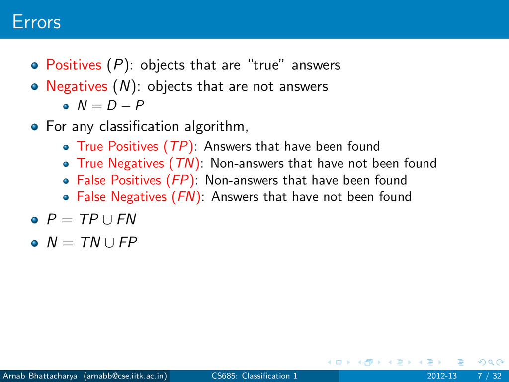
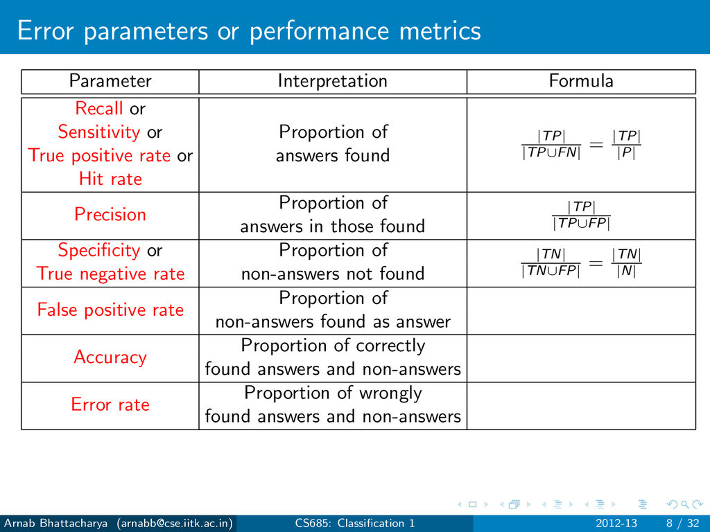
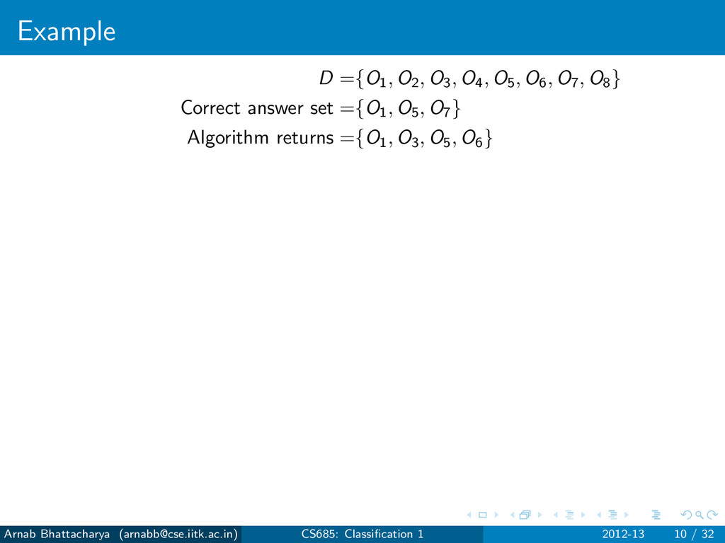
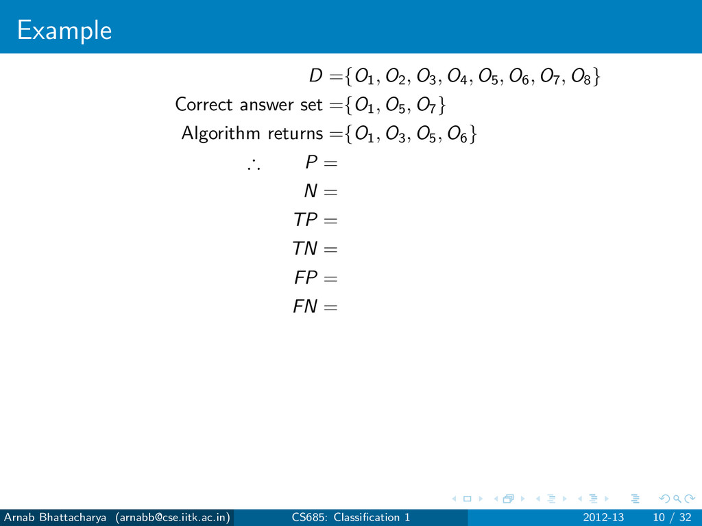
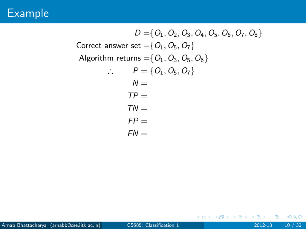
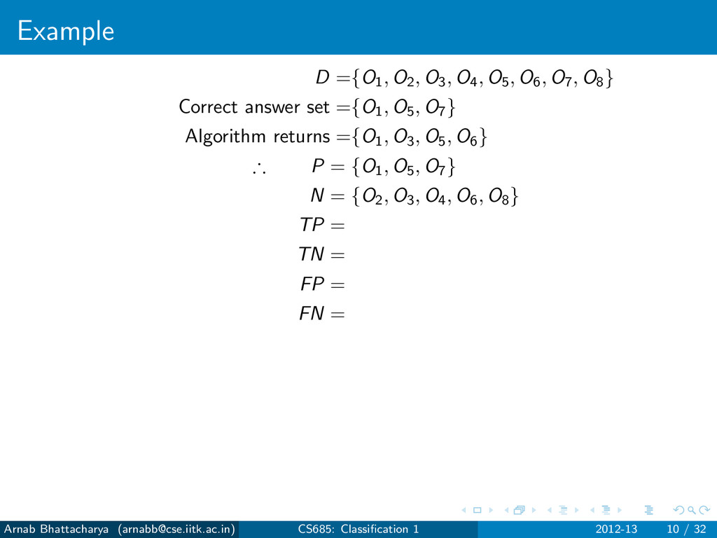
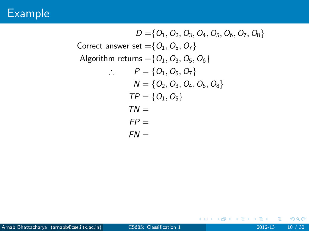
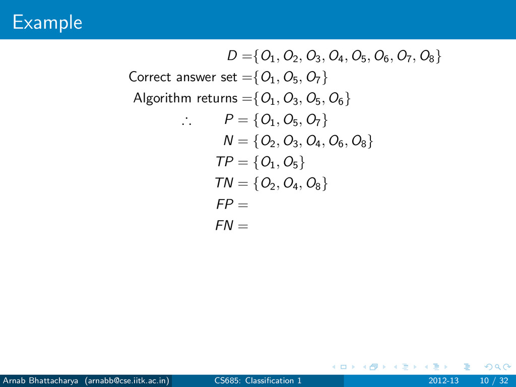
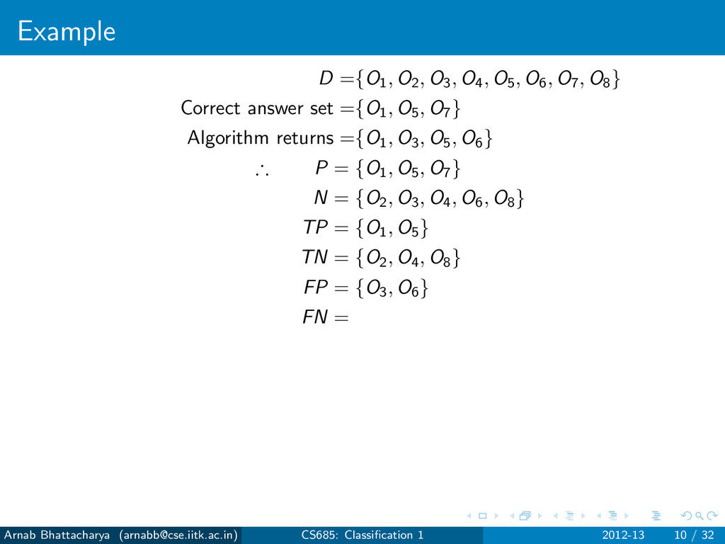
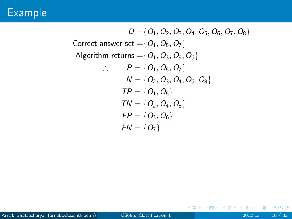
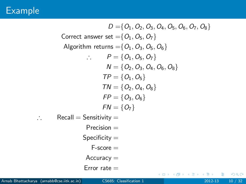
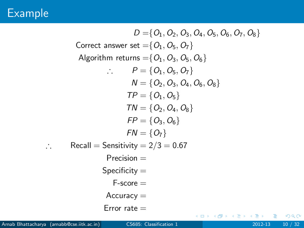
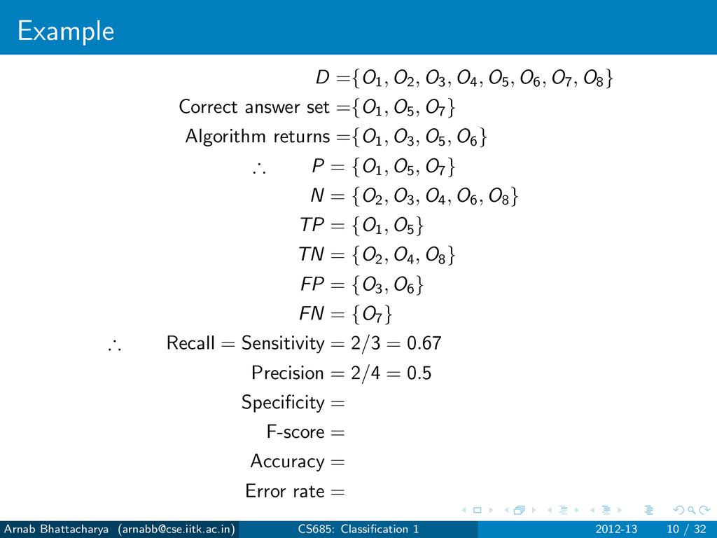
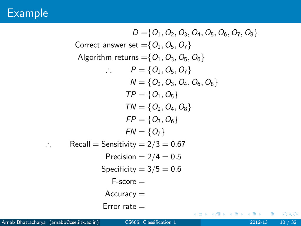
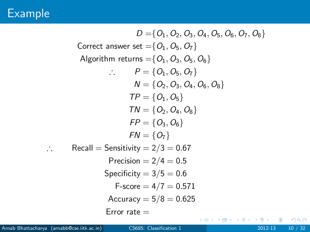
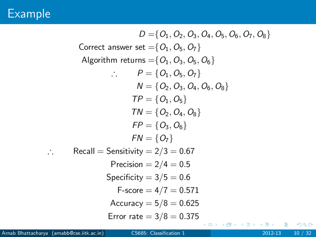
objects that are not answers N = D − P For any classification algorithm, True Positives (TP): Answers that have been found True Negatives (TN): Non-answers that have not been found False Positives (FP): Non-answers that have been found False Negatives (FN): Answers that have not been found P = TP ∪ FN N = TN ∪ FP Arnab Bhattacharya ([email protected]) CS685: Classification 1 2012-13 7 / 32
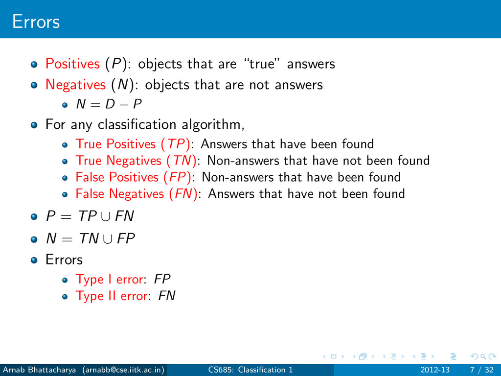
objects that are not answers N = D − P For any classification algorithm, True Positives (TP): Answers that have been found True Negatives (TN): Non-answers that have not been found False Positives (FP): Non-answers that have been found False Negatives (FN): Answers that have not been found P = TP ∪ FN N = TN ∪ FP Errors Type I error: FP Type II error: FN Arnab Bhattacharya ([email protected]) CS685: Classification 1 2012-13 7 / 32
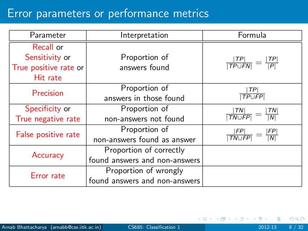
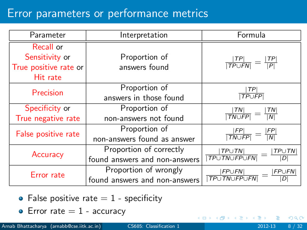
Sensitivity or Proportion of True positive rate or answers found Hit rate Precision Proportion of answers in those found Specificity or Proportion of True negative rate non-answers not found False positive rate Proportion of non-answers found as answer Accuracy Proportion of correctly found answers and non-answers Error rate Proportion of wrongly found answers and non-answers Arnab Bhattacharya ([email protected]) CS685: Classification 1 2012-13 8 / 32
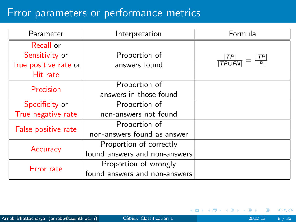
|TP| |TP∪FN| = |TP| |P| Sensitivity or Proportion of True positive rate or answers found Hit rate Precision Proportion of answers in those found Specificity or Proportion of True negative rate non-answers not found False positive rate Proportion of non-answers found as answer Accuracy Proportion of correctly found answers and non-answers Error rate Proportion of wrongly found answers and non-answers Arnab Bhattacharya ([email protected]) CS685: Classification 1 2012-13 8 / 32
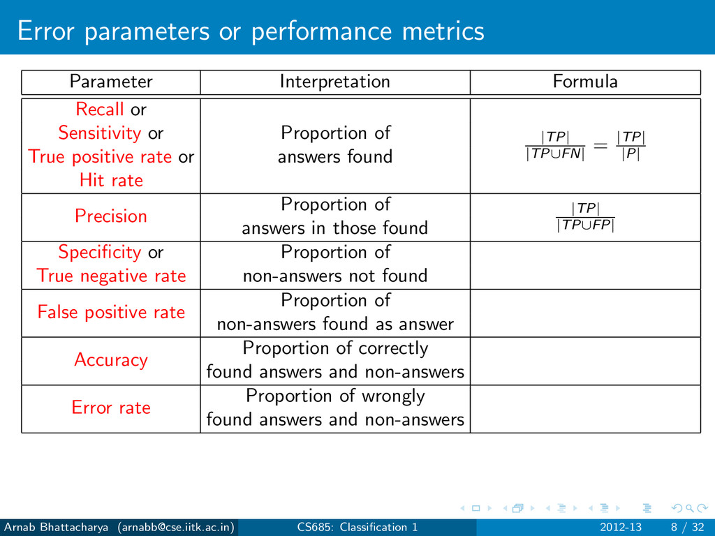
|TP| |TP∪FN| = |TP| |P| Sensitivity or Proportion of True positive rate or answers found Hit rate Precision Proportion of |TP| |TP∪FP| answers in those found Specificity or Proportion of True negative rate non-answers not found False positive rate Proportion of non-answers found as answer Accuracy Proportion of correctly found answers and non-answers Error rate Proportion of wrongly found answers and non-answers Arnab Bhattacharya ([email protected]) CS685: Classification 1 2012-13 8 / 32
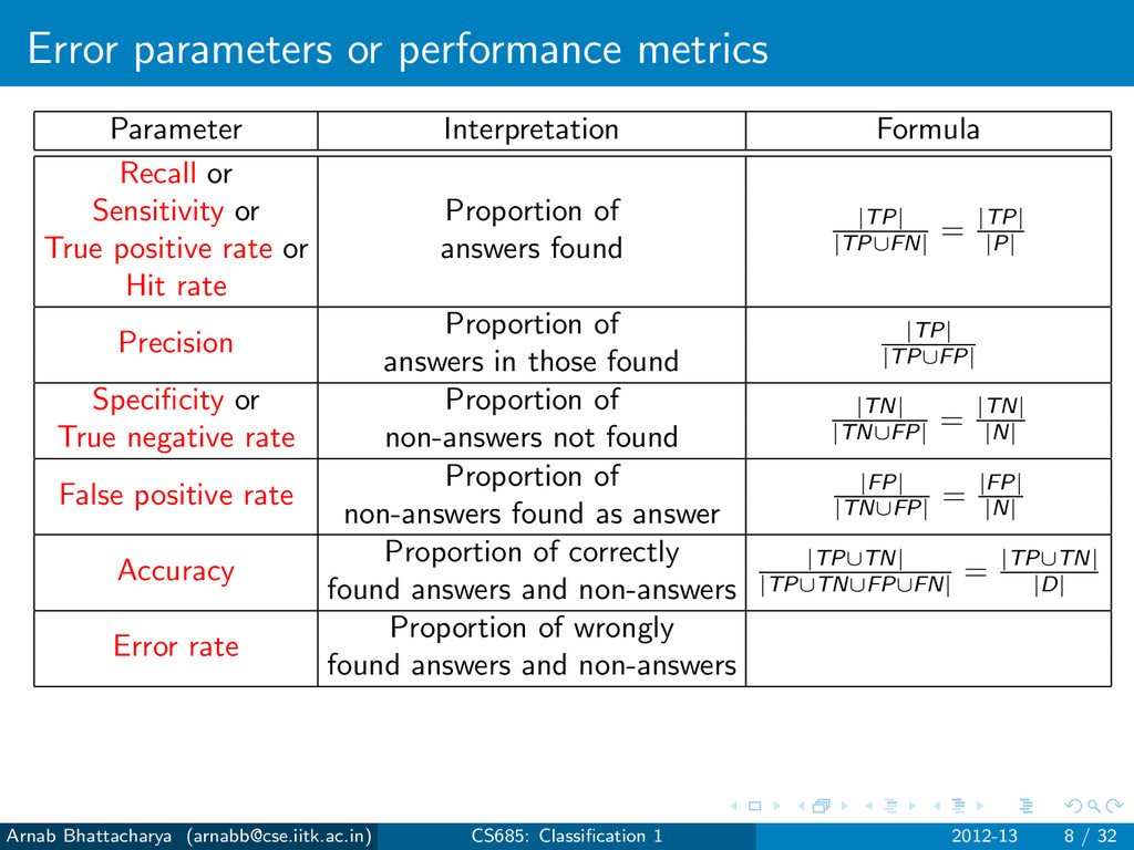
|TP| |TP∪FN| = |TP| |P| Sensitivity or Proportion of True positive rate or answers found Hit rate Precision Proportion of |TP| |TP∪FP| answers in those found Specificity or Proportion of |TN| |TN∪FP| = |TN| |N| True negative rate non-answers not found False positive rate Proportion of non-answers found as answer Accuracy Proportion of correctly found answers and non-answers Error rate Proportion of wrongly found answers and non-answers Arnab Bhattacharya ([email protected]) CS685: Classification 1 2012-13 8 / 32
|TP| |TP∪FN| = |TP| |P| Sensitivity or Proportion of True positive rate or answers found Hit rate Precision Proportion of |TP| |TP∪FP| answers in those found Specificity or Proportion of |TN| |TN∪FP| = |TN| |N| True negative rate non-answers not found False positive rate Proportion of |FP| |TN∪FP| = |FP| |N| non-answers found as answer Accuracy Proportion of correctly found answers and non-answers Error rate Proportion of wrongly found answers and non-answers Arnab Bhattacharya ([email protected]) CS685: Classification 1 2012-13 8 / 32
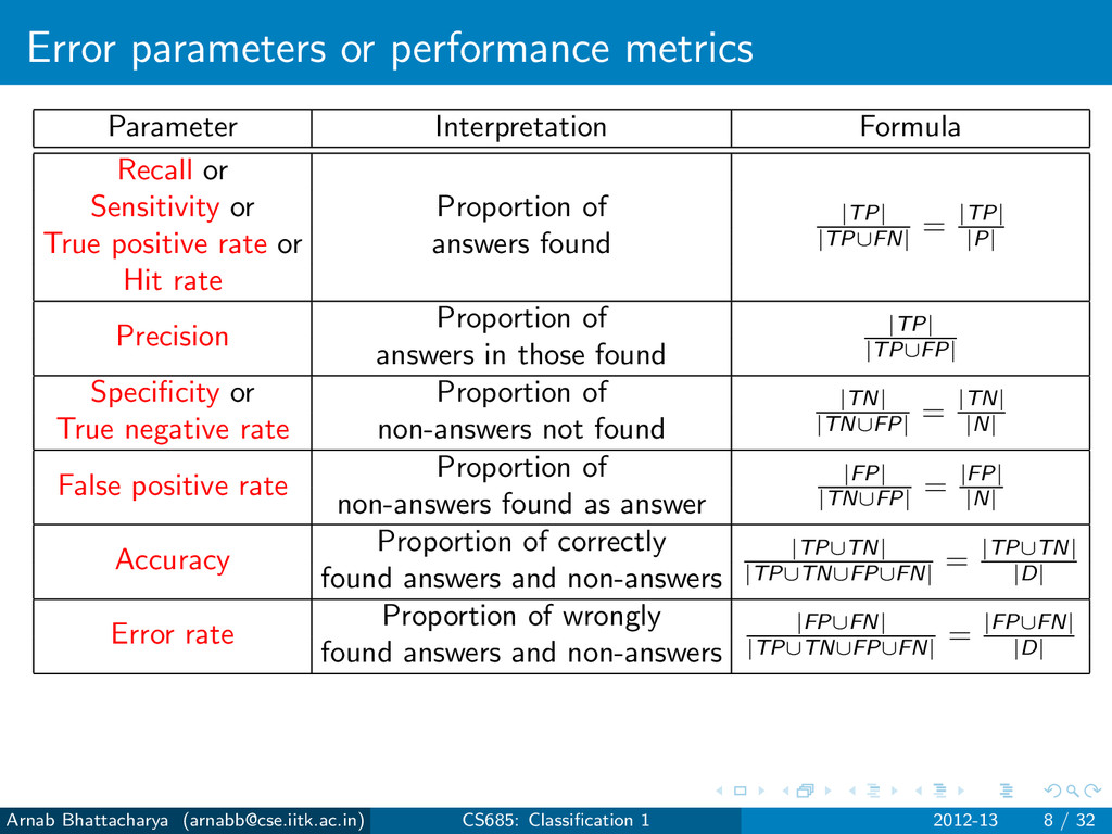
|TP| |TP∪FN| = |TP| |P| Sensitivity or Proportion of True positive rate or answers found Hit rate Precision Proportion of |TP| |TP∪FP| answers in those found Specificity or Proportion of |TN| |TN∪FP| = |TN| |N| True negative rate non-answers not found False positive rate Proportion of |FP| |TN∪FP| = |FP| |N| non-answers found as answer Accuracy Proportion of correctly |TP∪TN| |TP∪TN∪FP∪FN| = |TP∪TN| |D| found answers and non-answers Error rate Proportion of wrongly found answers and non-answers Arnab Bhattacharya ([email protected]) CS685: Classification 1 2012-13 8 / 32
|TP| |TP∪FN| = |TP| |P| Sensitivity or Proportion of True positive rate or answers found Hit rate Precision Proportion of |TP| |TP∪FP| answers in those found Specificity or Proportion of |TN| |TN∪FP| = |TN| |N| True negative rate non-answers not found False positive rate Proportion of |FP| |TN∪FP| = |FP| |N| non-answers found as answer Accuracy Proportion of correctly |TP∪TN| |TP∪TN∪FP∪FN| = |TP∪TN| |D| found answers and non-answers Error rate Proportion of wrongly |FP∪FN| |TP∪TN∪FP∪FN| = |FP∪FN| |D| found answers and non-answers Arnab Bhattacharya ([email protected]) CS685: Classification 1 2012-13 8 / 32
|TP| |TP∪FN| = |TP| |P| Sensitivity or Proportion of True positive rate or answers found Hit rate Precision Proportion of |TP| |TP∪FP| answers in those found Specificity or Proportion of |TN| |TN∪FP| = |TN| |N| True negative rate non-answers not found False positive rate Proportion of |FP| |TN∪FP| = |FP| |N| non-answers found as answer Accuracy Proportion of correctly |TP∪TN| |TP∪TN∪FP∪FN| = |TP∪TN| |D| found answers and non-answers Error rate Proportion of wrongly |FP∪FN| |TP∪TN∪FP∪FN| = |FP∪FN| |D| found answers and non-answers False positive rate = 1 - specificity Error rate = 1 - accuracy Arnab Bhattacharya ([email protected]) CS685: Classification 1 2012-13 8 / 32
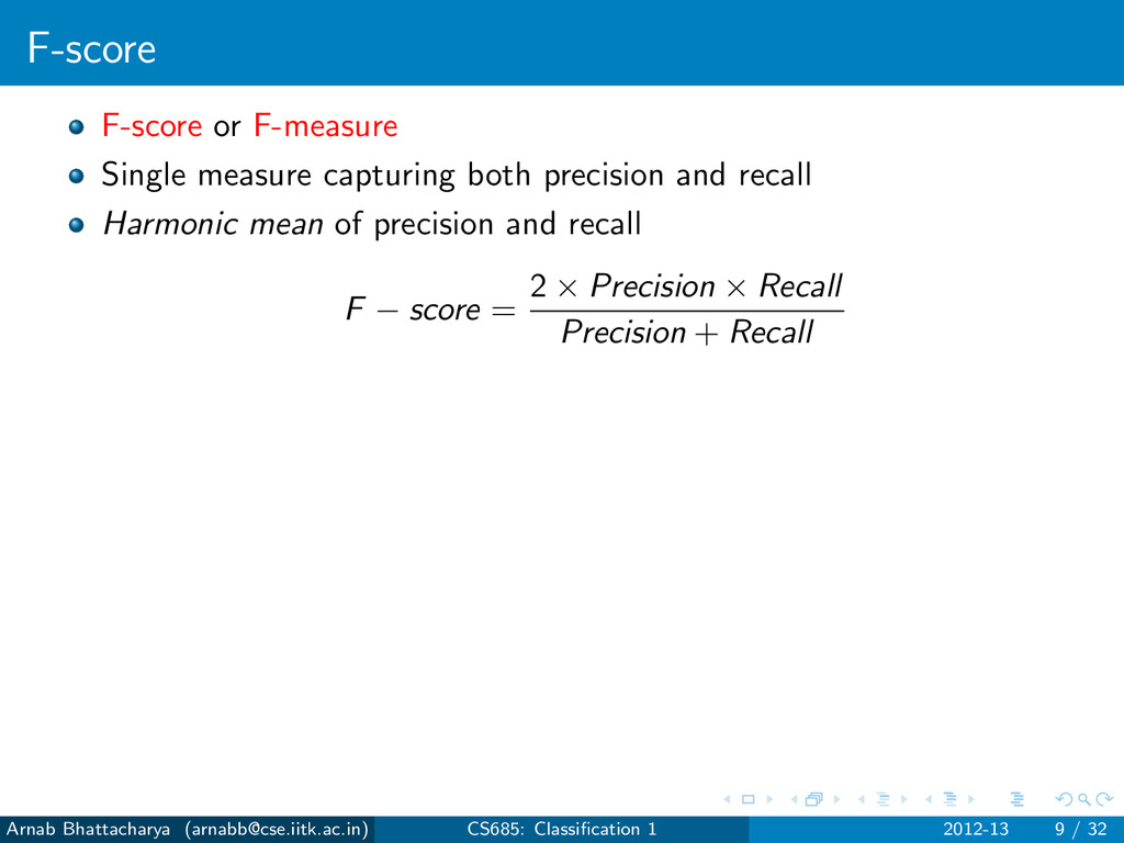
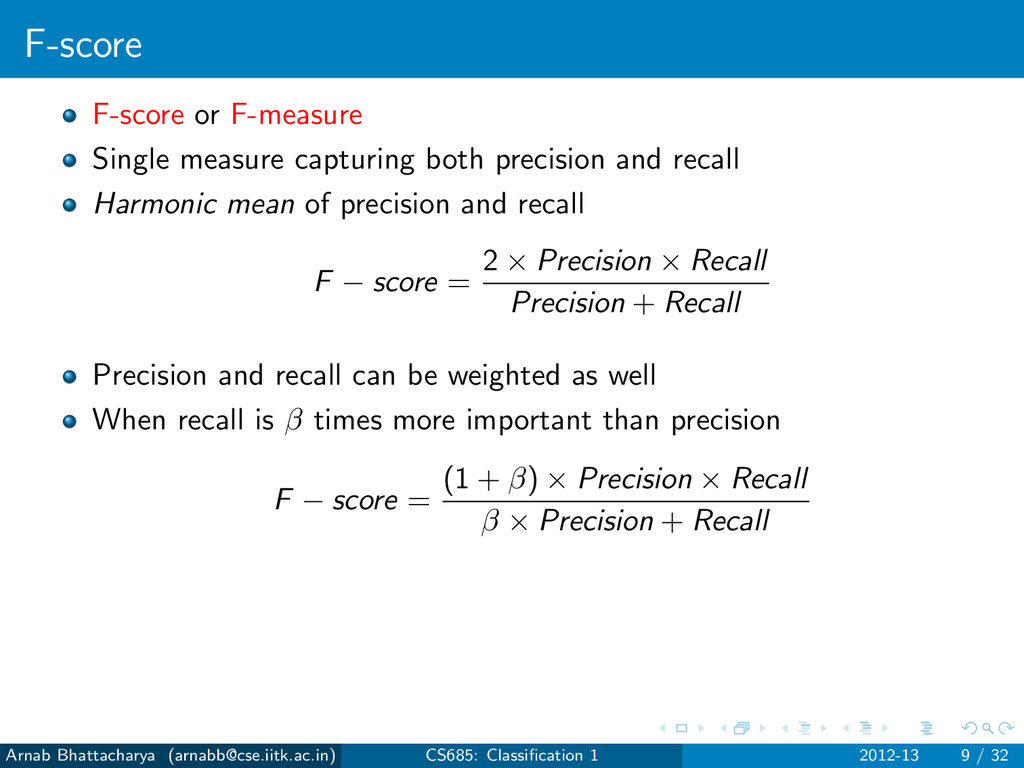
recall Harmonic mean of precision and recall F − score = 2 × Precision × Recall Precision + Recall Precision and recall can be weighted as well When recall is β times more important than precision F − score = (1 + β) × Precision × Recall β × Precision + Recall Arnab Bhattacharya ([email protected]) CS685: Classification 1 2012-13 9 / 32
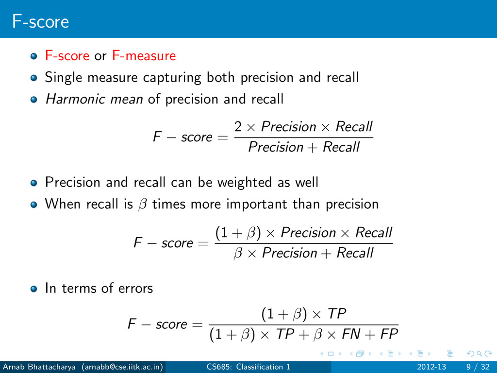
recall Harmonic mean of precision and recall F − score = 2 × Precision × Recall Precision + Recall Precision and recall can be weighted as well When recall is β times more important than precision F − score = (1 + β) × Precision × Recall β × Precision + Recall In terms of errors F − score = (1 + β) × TP (1 + β) × TP + β × FN + FP Arnab Bhattacharya ([email protected]) CS685: Classification 1 2012-13 9 / 32
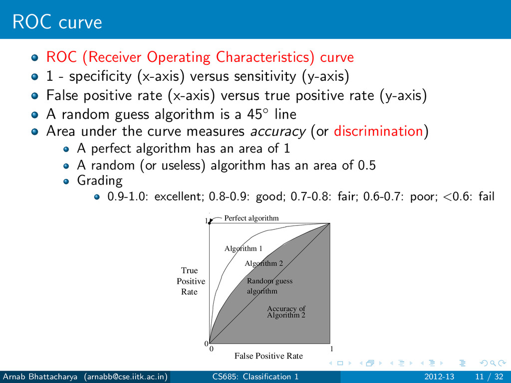
(x-axis) versus sensitivity (y-axis) False positive rate (x-axis) versus true positive rate (y-axis) A random guess algorithm is a 45◦ line Area under the curve measures accuracy (or discrimination) A perfect algorithm has an area of 1 A random (or useless) algorithm has an area of 0.5 Grading 0.9-1.0: excellent; 0.8-0.9: good; 0.7-0.8: fair; 0.6-0.7: poor; <0.6: fail Accuracy of Algorithm 2 True Positive Rate False Positive Rate 1 0 0 1 Algorithm 1 Algorithm 2 Perfect algorithm Random guess algorithm Arnab Bhattacharya ([email protected]) CS685: Classification 1 2012-13 11 / 32
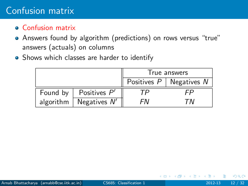
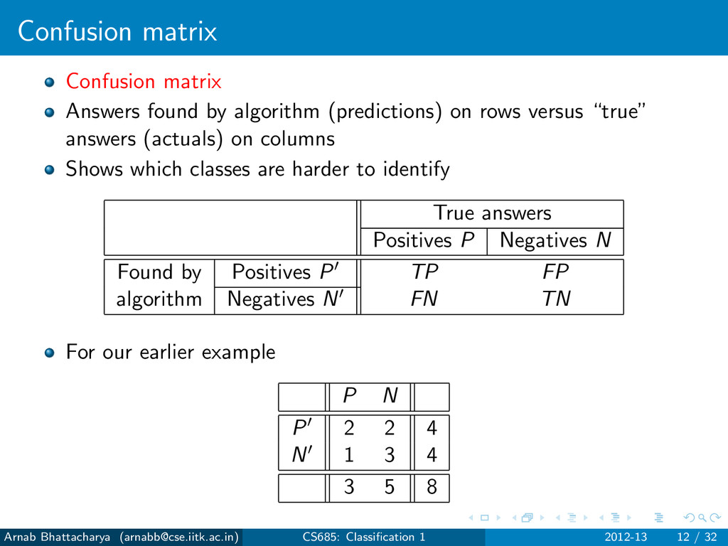
rows versus “true” answers (actuals) on columns Shows which classes are harder to identify True answers Positives P Negatives N Found by Positives P TP FP algorithm Negatives N FN TN Arnab Bhattacharya ([email protected]) CS685: Classification 1 2012-13 12 / 32
rows versus “true” answers (actuals) on columns Shows which classes are harder to identify True answers Positives P Negatives N Found by Positives P TP FP algorithm Negatives N FN TN For our earlier example P N P 2 2 4 N 1 3 4 3 5 8 Arnab Bhattacharya ([email protected]) CS685: Classification 1 2012-13 12 / 32
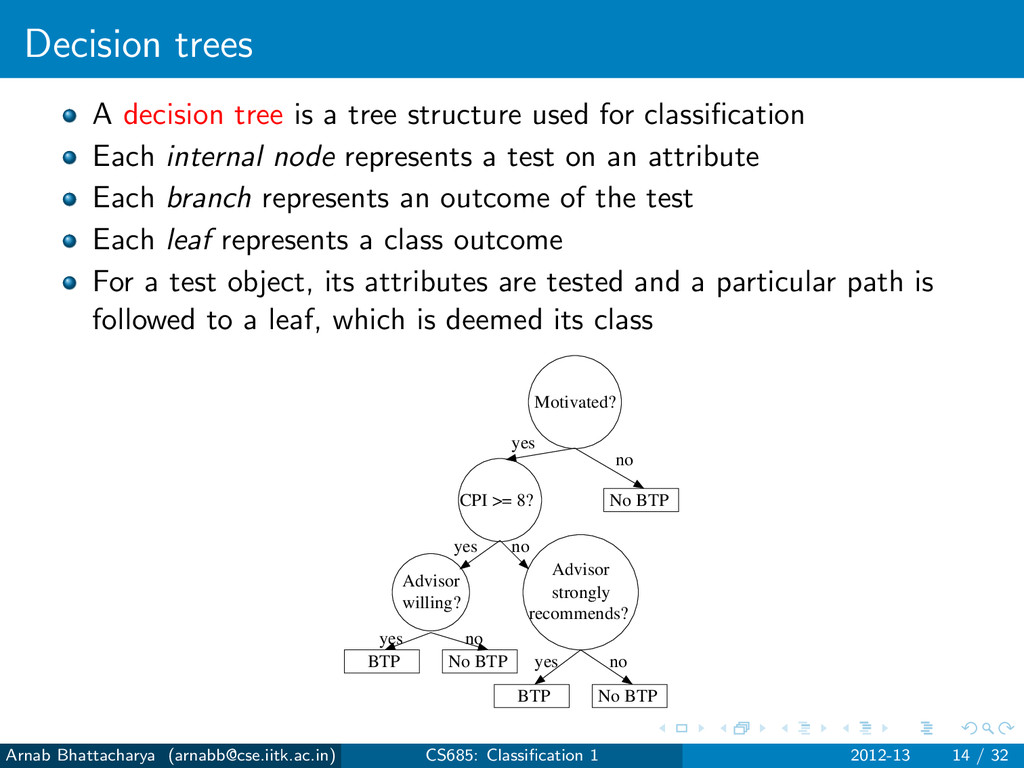
for classification Each internal node represents a test on an attribute Each branch represents an outcome of the test Each leaf represents a class outcome For a test object, its attributes are tested and a particular path is followed to a leaf, which is deemed its class Motivated? CPI >= 8? No BTP recommends? strongly Advisor Advisor willing? No BTP BTP No BTP BTP yes yes yes yes no no no no Arnab Bhattacharya ([email protected]) CS685: Classification 1 2012-13 14 / 32
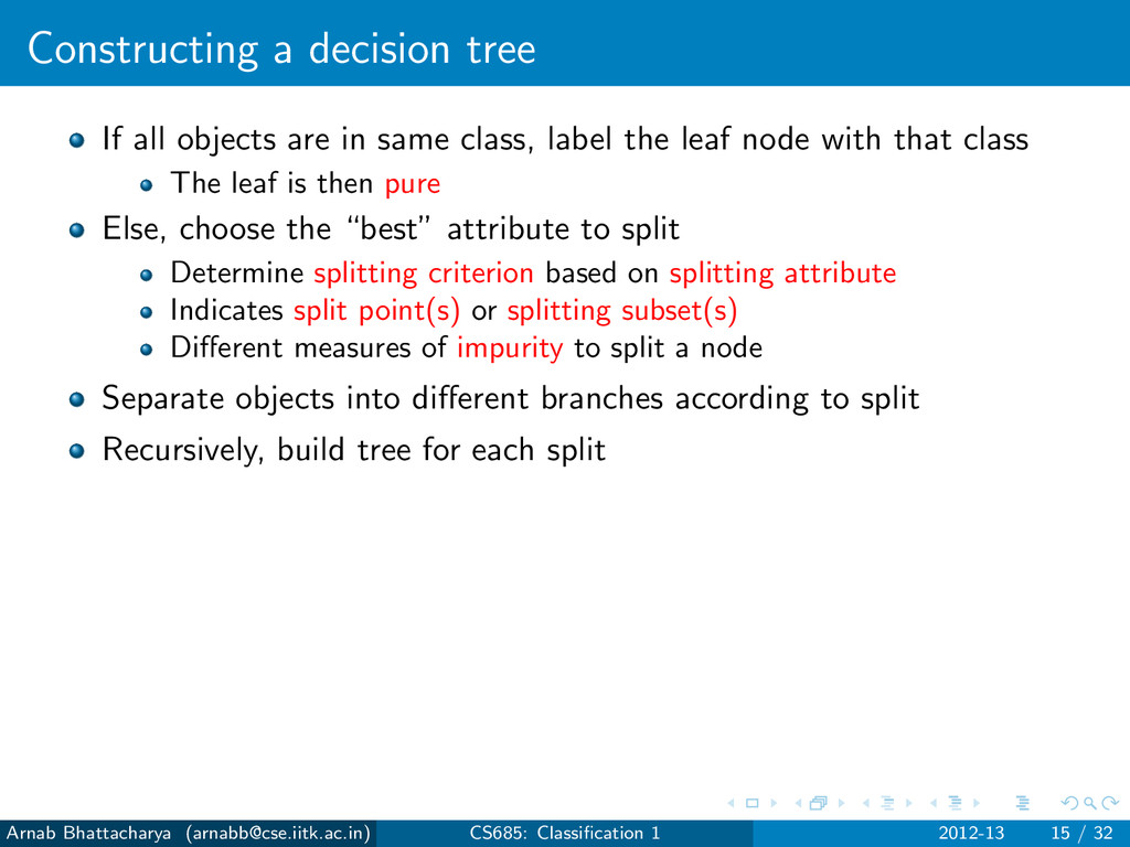
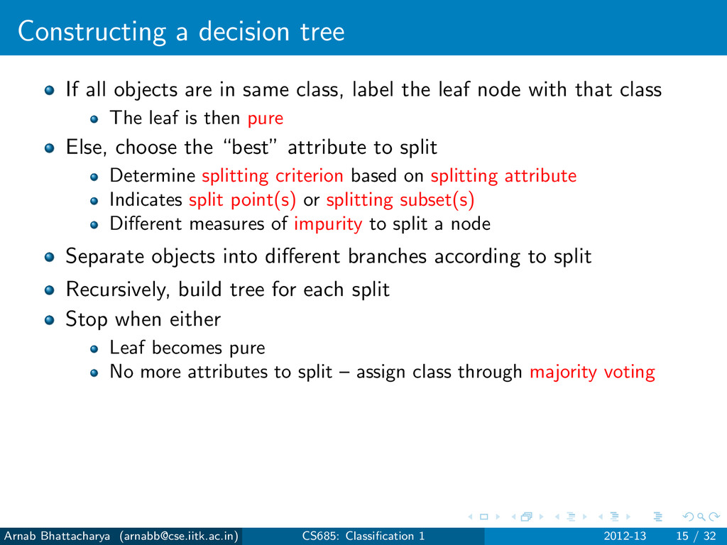
class, label the leaf node with that class The leaf is then pure Else, choose the “best” attribute to split Determine splitting criterion based on splitting attribute Indicates split point(s) or splitting subset(s) Different measures of impurity to split a node Separate objects into different branches according to split Recursively, build tree for each split Arnab Bhattacharya ([email protected]) CS685: Classification 1 2012-13 15 / 32
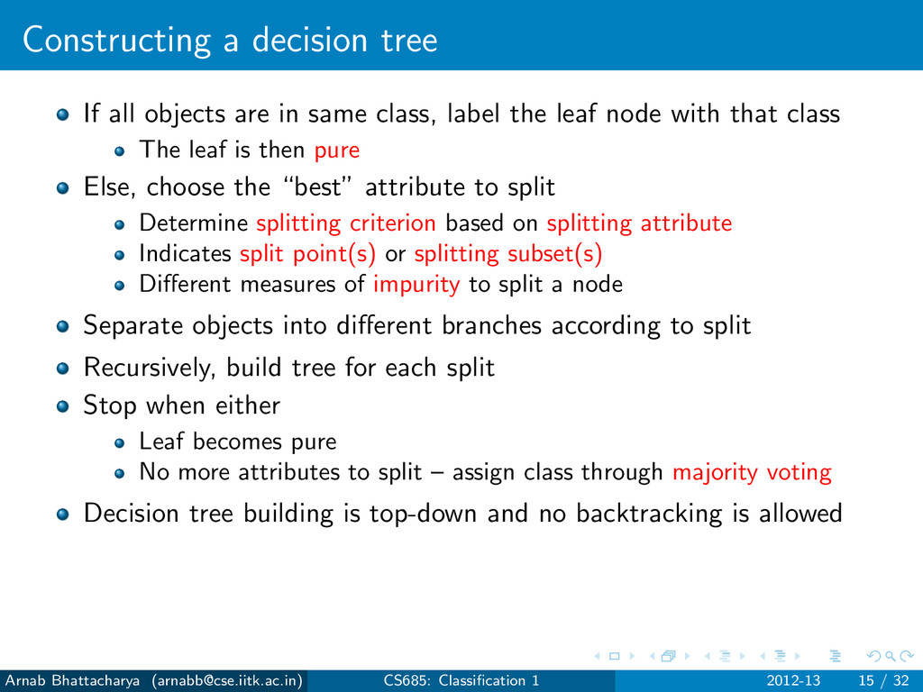
class, label the leaf node with that class The leaf is then pure Else, choose the “best” attribute to split Determine splitting criterion based on splitting attribute Indicates split point(s) or splitting subset(s) Different measures of impurity to split a node Separate objects into different branches according to split Recursively, build tree for each split Stop when either Leaf becomes pure No more attributes to split – assign class through majority voting Arnab Bhattacharya ([email protected]) CS685: Classification 1 2012-13 15 / 32
class, label the leaf node with that class The leaf is then pure Else, choose the “best” attribute to split Determine splitting criterion based on splitting attribute Indicates split point(s) or splitting subset(s) Different measures of impurity to split a node Separate objects into different branches according to split Recursively, build tree for each split Stop when either Leaf becomes pure No more attributes to split – assign class through majority voting Decision tree building is top-down and no backtracking is allowed Arnab Bhattacharya ([email protected]) CS685: Classification 1 2012-13 15 / 32
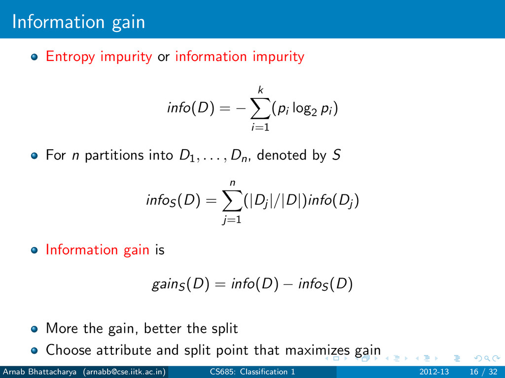
k i=1 (pi log2 pi ) For n partitions into D1, . . . , Dn, denoted by S infoS (D) = n j=1 (|Dj |/|D|)info(Dj ) Information gain is gainS (D) = info(D) − infoS (D) More the gain, better the split Choose attribute and split point that maximizes gain Arnab Bhattacharya ([email protected]) CS685: Classification 1 2012-13 16 / 32
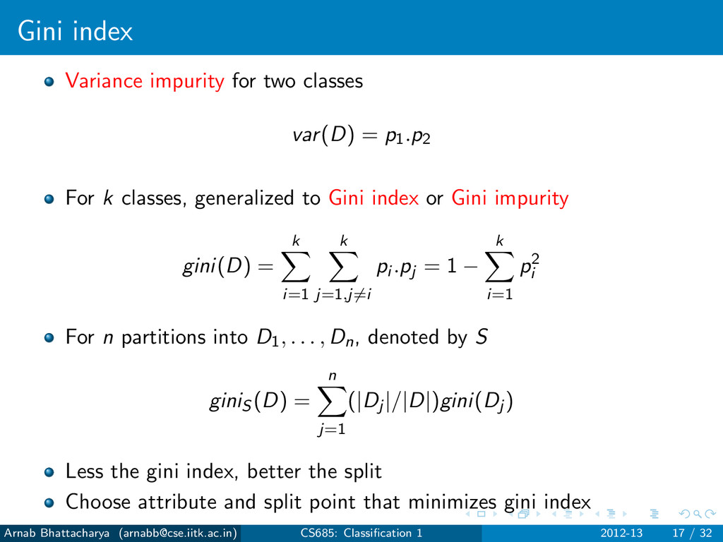
For k classes, generalized to Gini index or Gini impurity gini(D) = k i=1 k j=1,j=i pi .pj = 1 − k i=1 p2 i For n partitions into D1, . . . , Dn, denoted by S giniS (D) = n j=1 (|Dj |/|D|)gini(Dj ) Less the gini index, better the split Choose attribute and split point that minimizes gini index Arnab Bhattacharya ([email protected]) CS685: Classification 1 2012-13 17 / 32
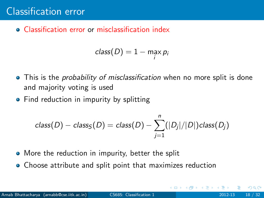
− max i pi This is the probability of misclassification when no more split is done and majority voting is used Find reduction in impurity by splitting class(D) − classS (D) = class(D) − n j=1 (|Dj |/|D|)class(Dj ) More the reduction in impurity, better the split Choose attribute and split point that maximizes reduction Arnab Bhattacharya ([email protected]) CS685: Classification 1 2012-13 18 / 32
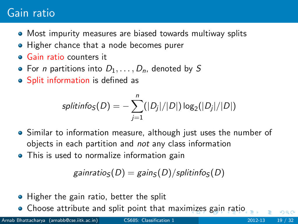
Higher chance that a node becomes purer Gain ratio counters it For n partitions into D1, . . . , Dn, denoted by S Split information is defined as splitinfoS (D) = − n j=1 (|Dj |/|D|) log2 (|Dj |/|D|) Similar to information measure, although just uses the number of objects in each partition and not any class information This is used to normalize information gain gainratioS (D) = gainS (D)/splitinfoS (D) Higher the gain ratio, better the split Choose attribute and split point that maximizes gain ratio Arnab Bhattacharya ([email protected]) CS685: Classification 1 2012-13 19 / 32
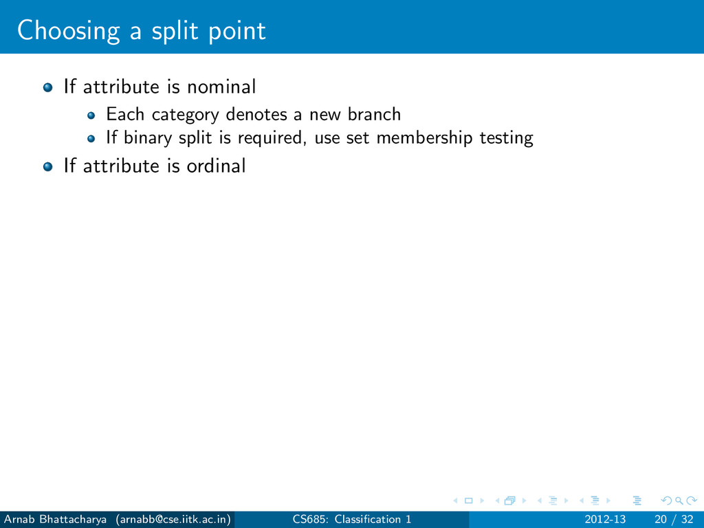
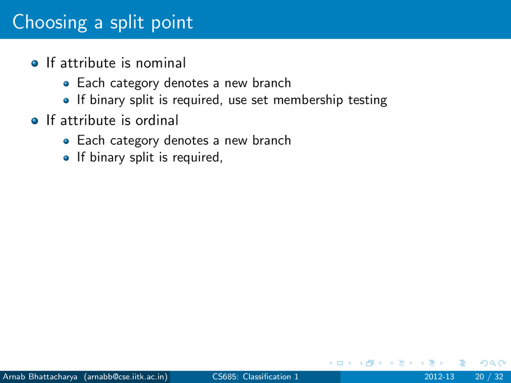
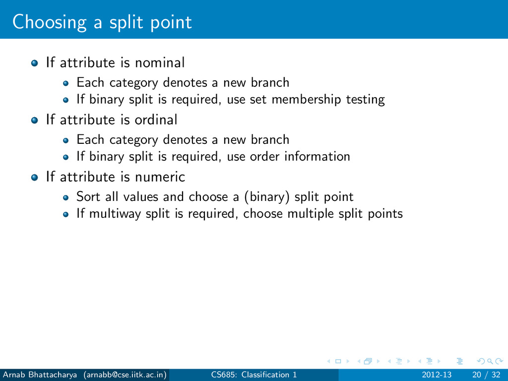
denotes a new branch If binary split is required, use set membership testing If attribute is ordinal Arnab Bhattacharya ([email protected]) CS685: Classification 1 2012-13 20 / 32
denotes a new branch If binary split is required, use set membership testing If attribute is ordinal Each category denotes a new branch If binary split is required, Arnab Bhattacharya ([email protected]) CS685: Classification 1 2012-13 20 / 32
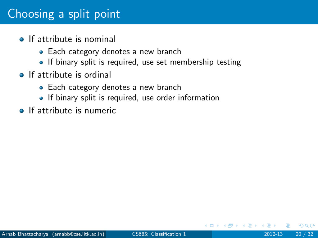
denotes a new branch If binary split is required, use set membership testing If attribute is ordinal Each category denotes a new branch If binary split is required, use order information If attribute is numeric Arnab Bhattacharya ([email protected]) CS685: Classification 1 2012-13 20 / 32
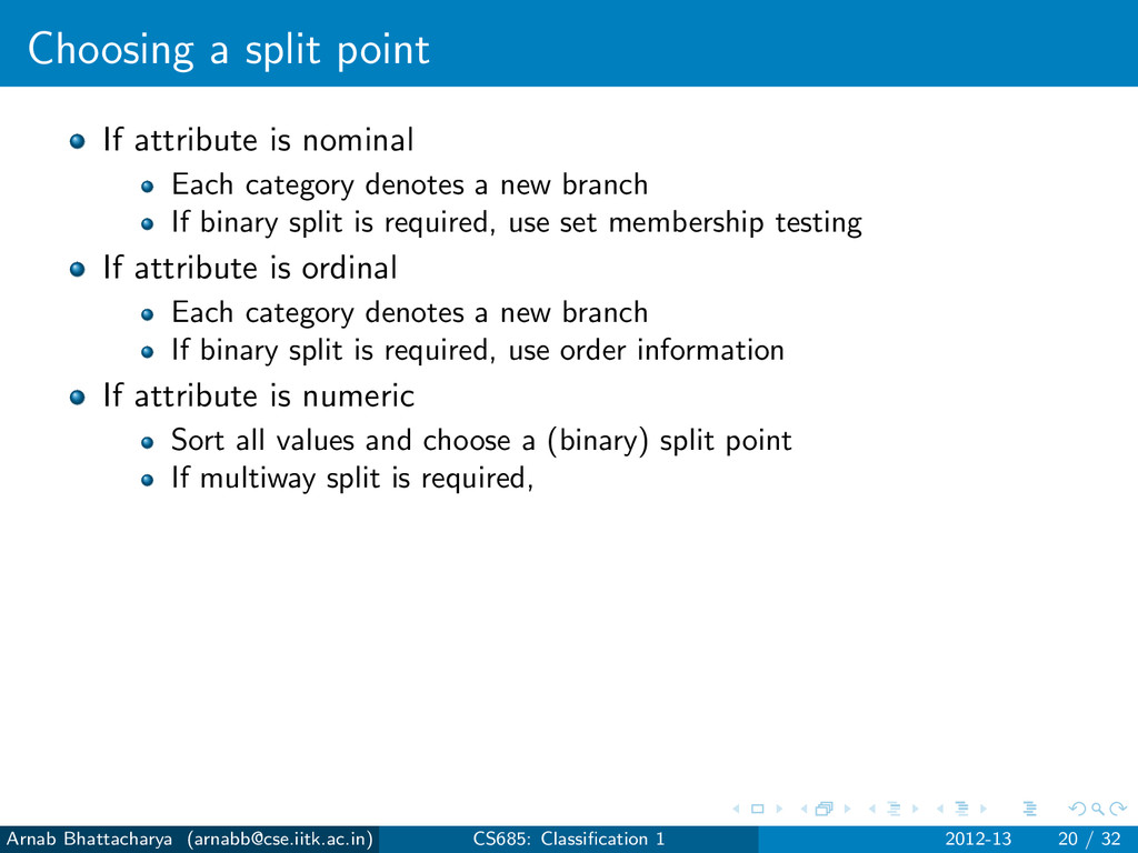
denotes a new branch If binary split is required, use set membership testing If attribute is ordinal Each category denotes a new branch If binary split is required, use order information If attribute is numeric Sort all values and choose a (binary) split point If multiway split is required, Arnab Bhattacharya ([email protected]) CS685: Classification 1 2012-13 20 / 32
denotes a new branch If binary split is required, use set membership testing If attribute is ordinal Each category denotes a new branch If binary split is required, use order information If attribute is numeric Sort all values and choose a (binary) split point If multiway split is required, choose multiple split points Arnab Bhattacharya ([email protected]) CS685: Classification 1 2012-13 20 / 32
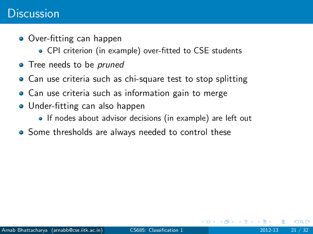
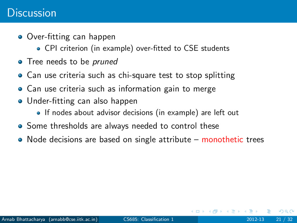
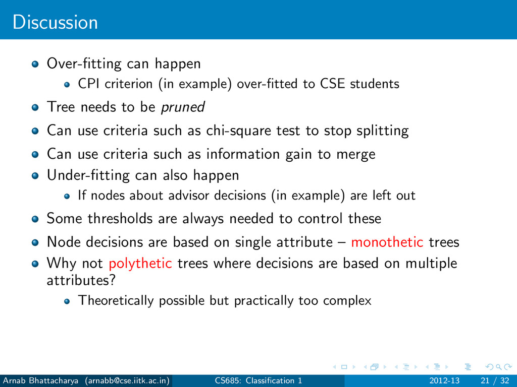
CSE students Tree needs to be pruned Can use criteria such as chi-square test to stop splitting Can use criteria such as information gain to merge Arnab Bhattacharya ([email protected]) CS685: Classification 1 2012-13 21 / 32
CSE students Tree needs to be pruned Can use criteria such as chi-square test to stop splitting Can use criteria such as information gain to merge Under-fitting can also happen If nodes about advisor decisions (in example) are left out Some thresholds are always needed to control these Arnab Bhattacharya ([email protected]) CS685: Classification 1 2012-13 21 / 32
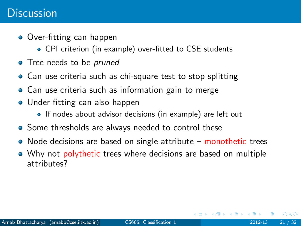
CSE students Tree needs to be pruned Can use criteria such as chi-square test to stop splitting Can use criteria such as information gain to merge Under-fitting can also happen If nodes about advisor decisions (in example) are left out Some thresholds are always needed to control these Node decisions are based on single attribute – monothetic trees Arnab Bhattacharya ([email protected]) CS685: Classification 1 2012-13 21 / 32
CSE students Tree needs to be pruned Can use criteria such as chi-square test to stop splitting Can use criteria such as information gain to merge Under-fitting can also happen If nodes about advisor decisions (in example) are left out Some thresholds are always needed to control these Node decisions are based on single attribute – monothetic trees Why not polythetic trees where decisions are based on multiple attributes? Arnab Bhattacharya ([email protected]) CS685: Classification 1 2012-13 21 / 32
CSE students Tree needs to be pruned Can use criteria such as chi-square test to stop splitting Can use criteria such as information gain to merge Under-fitting can also happen If nodes about advisor decisions (in example) are left out Some thresholds are always needed to control these Node decisions are based on single attribute – monothetic trees Why not polythetic trees where decisions are based on multiple attributes? Theoretically possible but practically too complex Arnab Bhattacharya ([email protected]) CS685: Classification 1 2012-13 21 / 32
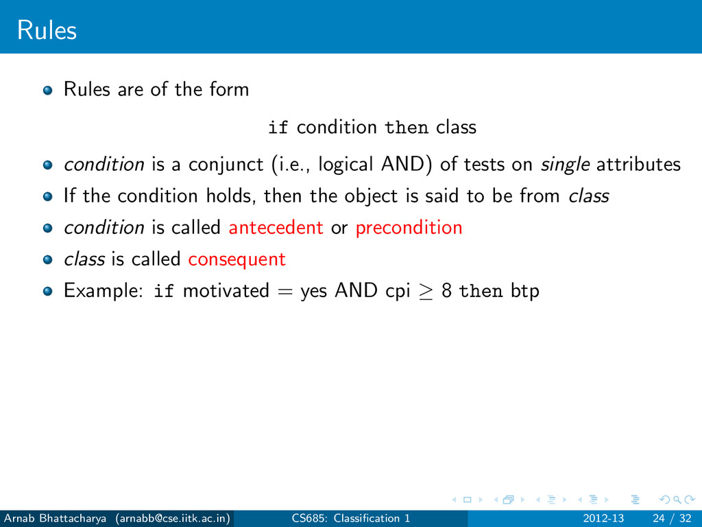
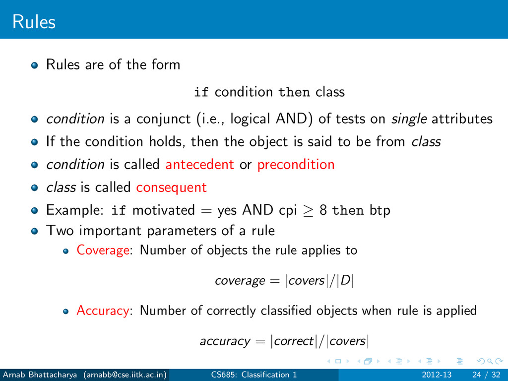
condition is a conjunct (i.e., logical AND) of tests on single attributes If the condition holds, then the object is said to be from class condition is called antecedent or precondition class is called consequent Example: if motivated = yes AND cpi ≥ 8 then btp Arnab Bhattacharya ([email protected]) CS685: Classification 1 2012-13 24 / 32
condition is a conjunct (i.e., logical AND) of tests on single attributes If the condition holds, then the object is said to be from class condition is called antecedent or precondition class is called consequent Example: if motivated = yes AND cpi ≥ 8 then btp Two important parameters of a rule Coverage: Number of objects the rule applies to coverage = |covers|/|D| Accuracy: Number of correctly classified objects when rule is applied accuracy = |correct|/|covers| Arnab Bhattacharya ([email protected]) CS685: Classification 1 2012-13 24 / 32
that satisfies it is “triggered” If for that tuple, it is the only rule, then it is “fired” Arnab Bhattacharya ([email protected]) CS685: Classification 1 2012-13 25 / 32
that satisfies it is “triggered” If for that tuple, it is the only rule, then it is “fired” Otherwise, a conflict resolution strategy is devised Arnab Bhattacharya ([email protected]) CS685: Classification 1 2012-13 25 / 32
that satisfies it is “triggered” If for that tuple, it is the only rule, then it is “fired” Otherwise, a conflict resolution strategy is devised Size-based ordering: Rule with larger antecedent is invoked More stringent, i.e., tougher Arnab Bhattacharya ([email protected]) CS685: Classification 1 2012-13 25 / 32
that satisfies it is “triggered” If for that tuple, it is the only rule, then it is “fired” Otherwise, a conflict resolution strategy is devised Size-based ordering: Rule with larger antecedent is invoked More stringent, i.e., tougher Class-based ordering: Two schemes Consequent class is more frequent, i.e., according to order of prevalence Consequent class has less misclassification Within same class, there is arbitrary ordering Arnab Bhattacharya ([email protected]) CS685: Classification 1 2012-13 25 / 32
that satisfies it is “triggered” If for that tuple, it is the only rule, then it is “fired” Otherwise, a conflict resolution strategy is devised Size-based ordering: Rule with larger antecedent is invoked More stringent, i.e., tougher Class-based ordering: Two schemes Consequent class is more frequent, i.e., according to order of prevalence Consequent class has less misclassification Within same class, there is arbitrary ordering Rule-based ordering: Priority list according to some function based on coverage, accuracy and size Arnab Bhattacharya ([email protected]) CS685: Classification 1 2012-13 25 / 32
that satisfies it is “triggered” If for that tuple, it is the only rule, then it is “fired” Otherwise, a conflict resolution strategy is devised Size-based ordering: Rule with larger antecedent is invoked More stringent, i.e., tougher Class-based ordering: Two schemes Consequent class is more frequent, i.e., according to order of prevalence Consequent class has less misclassification Within same class, there is arbitrary ordering Rule-based ordering: Priority list according to some function based on coverage, accuracy and size For a query tuple, the first rule that satisifies it is invoked If no such rule, then a default rule is invoked: if () then class i Class i is the most abundant class Arnab Bhattacharya ([email protected]) CS685: Classification 1 2012-13 25 / 32
rule As verbose or complex as the decision tree itself Rules are mutually exclusive and exhaustive Arnab Bhattacharya ([email protected]) CS685: Classification 1 2012-13 26 / 32
rule As verbose or complex as the decision tree itself Rules are mutually exclusive and exhaustive No need to order the rules Arnab Bhattacharya ([email protected]) CS685: Classification 1 2012-13 26 / 32
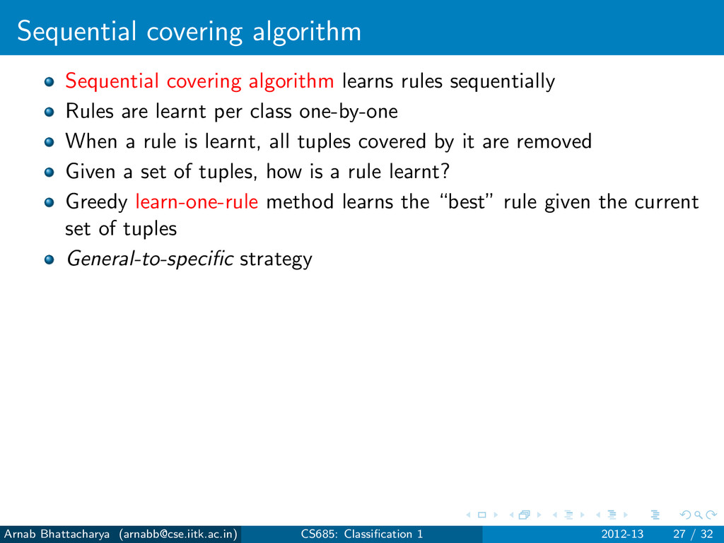
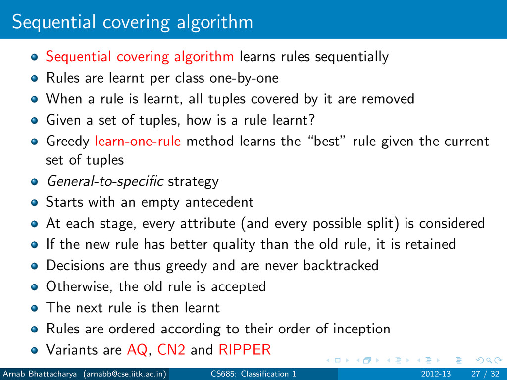
are learnt per class one-by-one When a rule is learnt, all tuples covered by it are removed Given a set of tuples, how is a rule learnt? Arnab Bhattacharya ([email protected]) CS685: Classification 1 2012-13 27 / 32
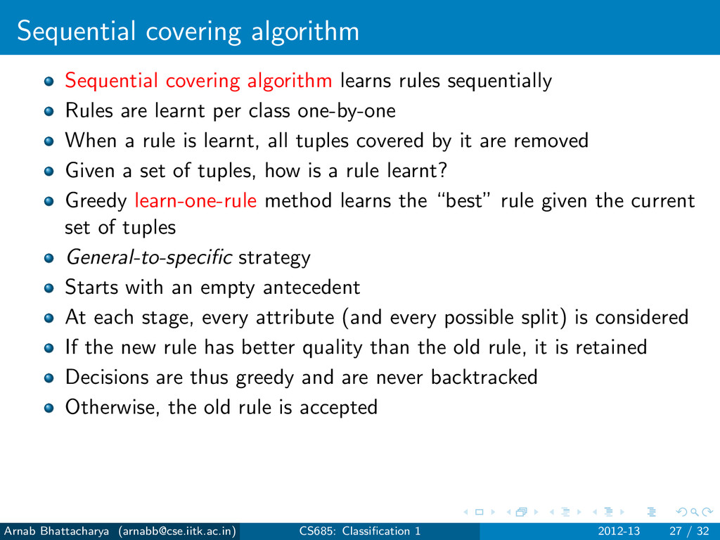
are learnt per class one-by-one When a rule is learnt, all tuples covered by it are removed Given a set of tuples, how is a rule learnt? Greedy learn-one-rule method learns the “best” rule given the current set of tuples General-to-specific strategy Arnab Bhattacharya ([email protected]) CS685: Classification 1 2012-13 27 / 32
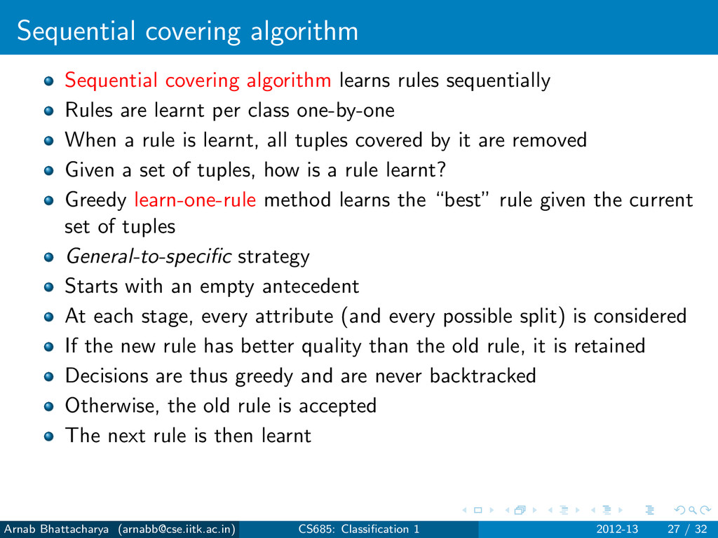
are learnt per class one-by-one When a rule is learnt, all tuples covered by it are removed Given a set of tuples, how is a rule learnt? Greedy learn-one-rule method learns the “best” rule given the current set of tuples General-to-specific strategy Starts with an empty antecedent At each stage, every attribute (and every possible split) is considered If the new rule has better quality than the old rule, it is retained Decisions are thus greedy and are never backtracked Otherwise, the old rule is accepted Arnab Bhattacharya ([email protected]) CS685: Classification 1 2012-13 27 / 32
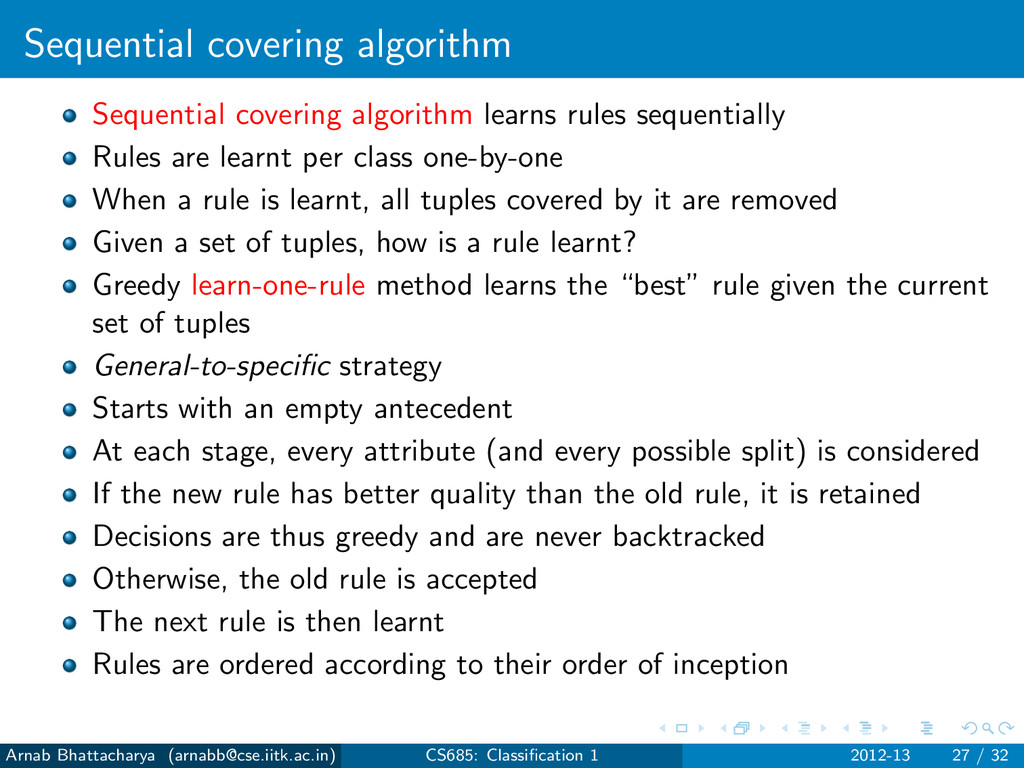
are learnt per class one-by-one When a rule is learnt, all tuples covered by it are removed Given a set of tuples, how is a rule learnt? Greedy learn-one-rule method learns the “best” rule given the current set of tuples General-to-specific strategy Starts with an empty antecedent At each stage, every attribute (and every possible split) is considered If the new rule has better quality than the old rule, it is retained Decisions are thus greedy and are never backtracked Otherwise, the old rule is accepted The next rule is then learnt Arnab Bhattacharya ([email protected]) CS685: Classification 1 2012-13 27 / 32
are learnt per class one-by-one When a rule is learnt, all tuples covered by it are removed Given a set of tuples, how is a rule learnt? Greedy learn-one-rule method learns the “best” rule given the current set of tuples General-to-specific strategy Starts with an empty antecedent At each stage, every attribute (and every possible split) is considered If the new rule has better quality than the old rule, it is retained Decisions are thus greedy and are never backtracked Otherwise, the old rule is accepted The next rule is then learnt Rules are ordered according to their order of inception Arnab Bhattacharya ([email protected]) CS685: Classification 1 2012-13 27 / 32
are learnt per class one-by-one When a rule is learnt, all tuples covered by it are removed Given a set of tuples, how is a rule learnt? Greedy learn-one-rule method learns the “best” rule given the current set of tuples General-to-specific strategy Starts with an empty antecedent At each stage, every attribute (and every possible split) is considered If the new rule has better quality than the old rule, it is retained Decisions are thus greedy and are never backtracked Otherwise, the old rule is accepted The next rule is then learnt Rules are ordered according to their order of inception Variants are AQ, CN2 and RIPPER Arnab Bhattacharya ([email protected]) CS685: Classification 1 2012-13 27 / 32
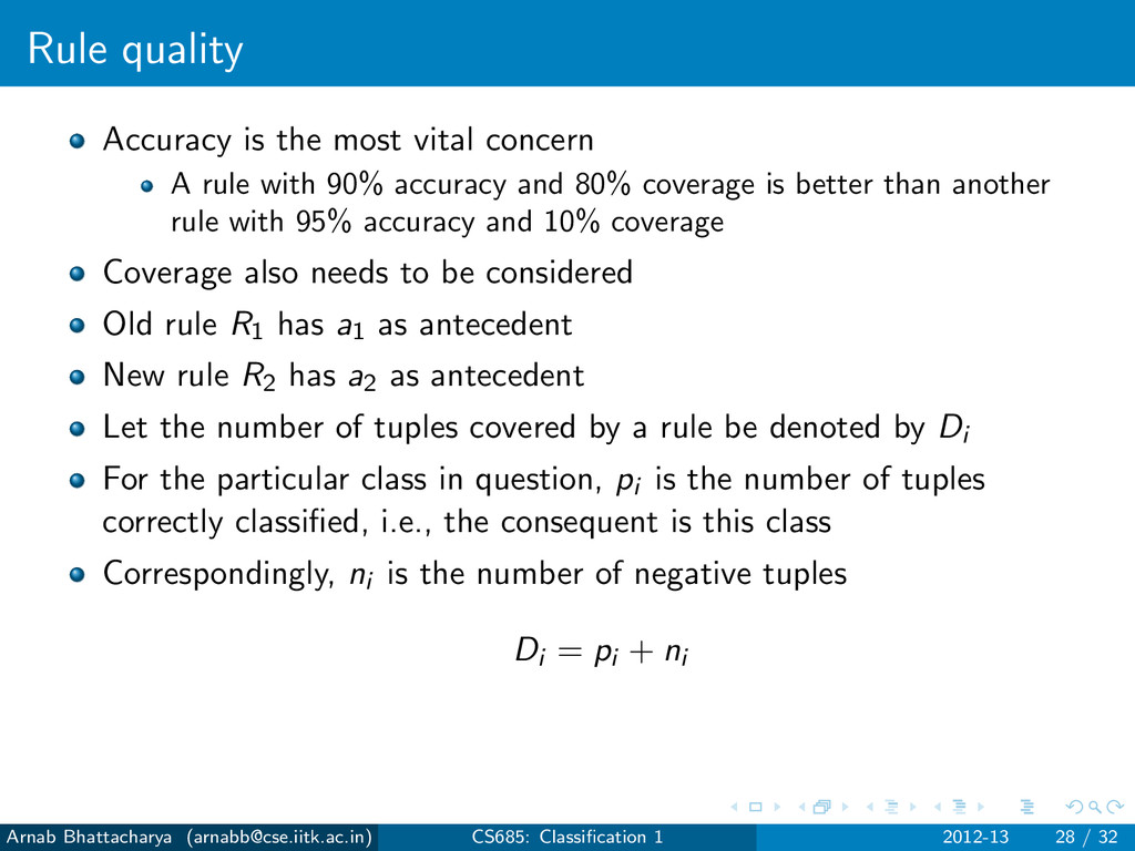
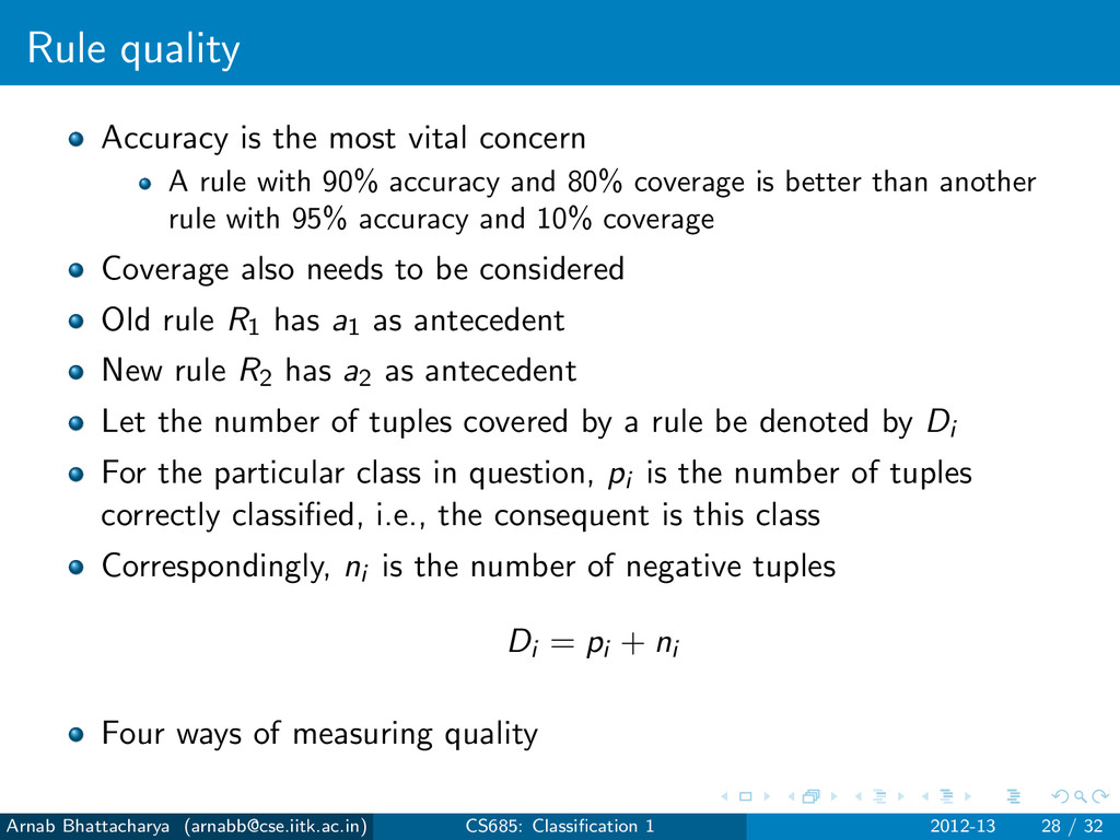
with 90% accuracy and 80% coverage is better than another rule with 95% accuracy and 10% coverage Coverage also needs to be considered Arnab Bhattacharya ([email protected]) CS685: Classification 1 2012-13 28 / 32
with 90% accuracy and 80% coverage is better than another rule with 95% accuracy and 10% coverage Coverage also needs to be considered Old rule R1 has a1 as antecedent New rule R2 has a2 as antecedent Let the number of tuples covered by a rule be denoted by Di For the particular class in question, pi is the number of tuples correctly classified, i.e., the consequent is this class Correspondingly, ni is the number of negative tuples Di = pi + ni Arnab Bhattacharya ([email protected]) CS685: Classification 1 2012-13 28 / 32
with 90% accuracy and 80% coverage is better than another rule with 95% accuracy and 10% coverage Coverage also needs to be considered Old rule R1 has a1 as antecedent New rule R2 has a2 as antecedent Let the number of tuples covered by a rule be denoted by Di For the particular class in question, pi is the number of tuples correctly classified, i.e., the consequent is this class Correspondingly, ni is the number of negative tuples Di = pi + ni Four ways of measuring quality Arnab Bhattacharya ([email protected]) CS685: Classification 1 2012-13 28 / 32
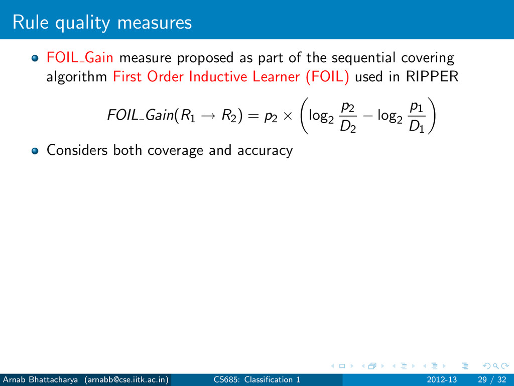
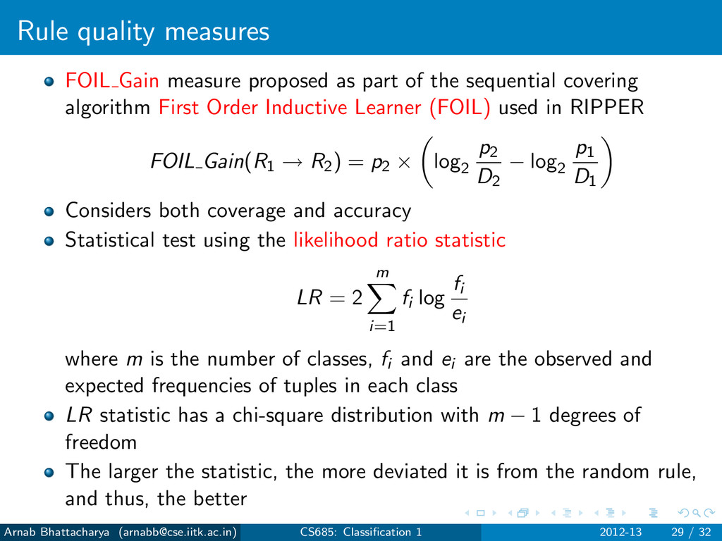
the sequential covering algorithm First Order Inductive Learner (FOIL) used in RIPPER FOIL Gain(R1 → R2) = p2 × log2 p2 D2 − log2 p1 D1 Considers both coverage and accuracy Statistical test using the likelihood ratio statistic LR = 2 m i=1 fi log fi ei where m is the number of classes, fi and ei are the observed and expected frequencies of tuples in each class LR statistic has a chi-square distribution with m − 1 degrees of freedom The larger the statistic, the more deviated it is from the random rule, and thus, the better Arnab Bhattacharya ([email protected]) CS685: Classification 1 2012-13 29 / 32
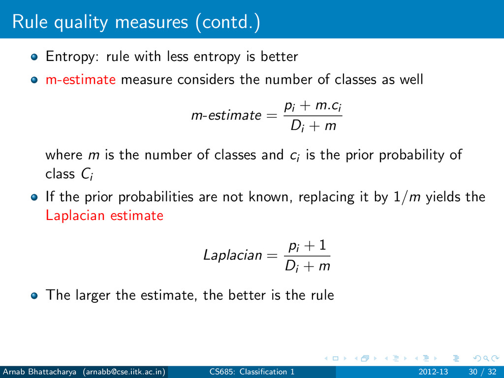
better m-estimate measure considers the number of classes as well m-estimate = pi + m.ci Di + m where m is the number of classes and ci is the prior probability of class Ci If the prior probabilities are not known, replacing it by 1/m yields the Laplacian estimate Laplacian = pi + 1 Di + m The larger the estimate, the better is the rule Arnab Bhattacharya ([email protected]) CS685: Classification 1 2012-13 30 / 32
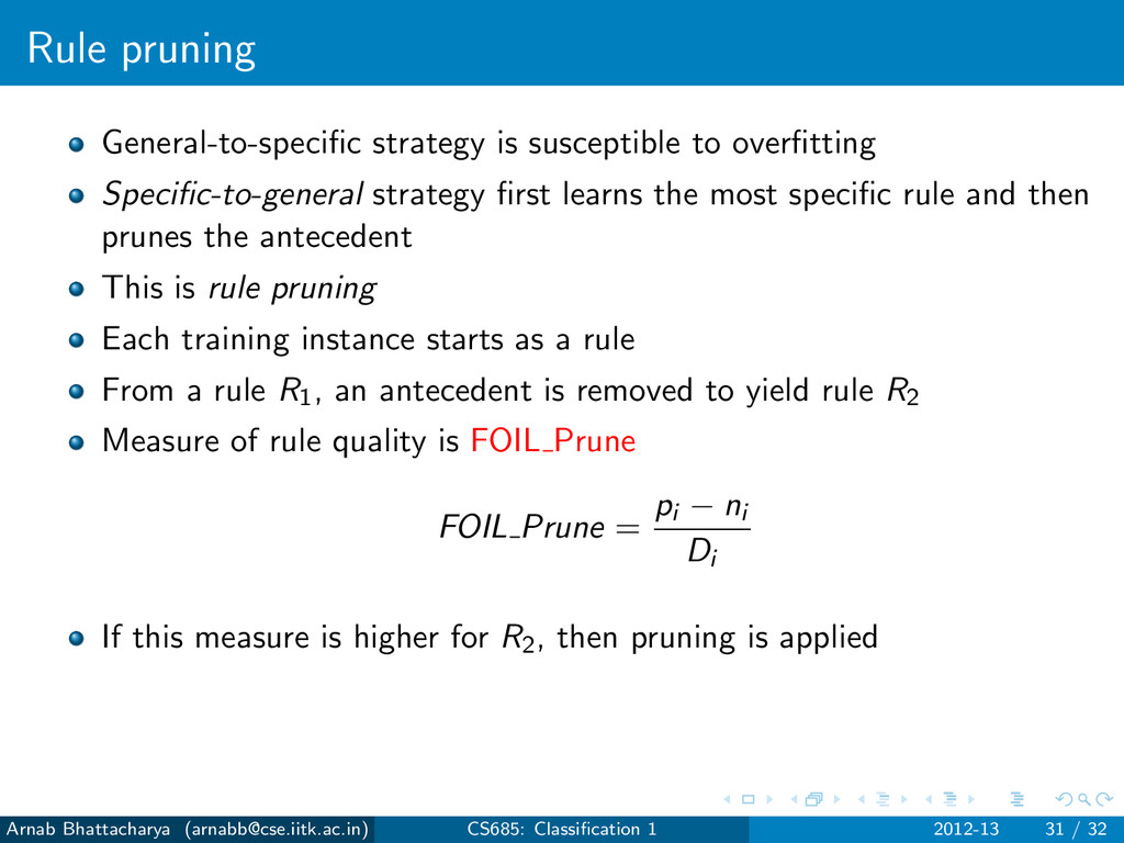
first learns the most specific rule and then prunes the antecedent This is rule pruning Arnab Bhattacharya ([email protected]) CS685: Classification 1 2012-13 31 / 32
first learns the most specific rule and then prunes the antecedent This is rule pruning Each training instance starts as a rule From a rule R1, an antecedent is removed to yield rule R2 Measure of rule quality is FOIL Prune FOIL Prune = pi − ni Di If this measure is higher for R2, then pruning is applied Arnab Bhattacharya ([email protected]) CS685: Classification 1 2012-13 31 / 32
learn rectilinear boundaries Rules have an interpretation and can lead to descriptive models Arnab Bhattacharya ([email protected]) CS685: Classification 1 2012-13 32 / 32
learn rectilinear boundaries Rules have an interpretation and can lead to descriptive models Can handle imbalance in class distribution very well Arnab Bhattacharya ([email protected]) CS685: Classification 1 2012-13 32 / 32
![CS685: Data Mining Classification Arnab Bhattacharya [email protected] Computer Science and](https://files.speakerdeck.com/presentations/505bedb50fb5de000202977f/slide_0.jpg)
![Learning rules from a decision tree Arnab Bhattacharya ([email protected]) CS685:](https://files.speakerdeck.com/presentations/505bedb50fb5de000202977f/slide_78.jpg)
![Discussion Rules can be very verbose Arnab Bhattacharya ([email protected]) CS685:](https://files.speakerdeck.com/presentations/505bedb50fb5de000202977f/slide_99.jpg)