CS685 Data Preprocessing 1

Transcript

1. CS685: Data Mining Data Preprocessing Arnab Bhattacharya arnabb@cse.iitk.ac.in Computer Science and Engineering, Indian Institute of Technology, Kanpur http://web.cse.iitk.ac.in/~cs685/ 1st semester, 2012-13 Tue, Wed, Fri 0900-1000 at CS101 Arnab Bhattacharya (arnabb@cse.iitk.ac.in) CS685: Preprocessing 1 2012-13 1 / 43
2. Outline 1 Data 2 Data preprocessing 3 Data cleaning 4 Data reduction Dimensionality reduction Numerosity reduction Arnab Bhattacharya (arnabb@cse.iitk.ac.in) CS685: Preprocessing 1 2012-13 2 / 43
3. Outline 1 Data 2 Data preprocessing 3 Data cleaning 4 Data reduction Dimensionality reduction Numerosity reduction Arnab Bhattacharya (arnabb@cse.iitk.ac.in) CS685: Preprocessing 1 2012-13 3 / 43
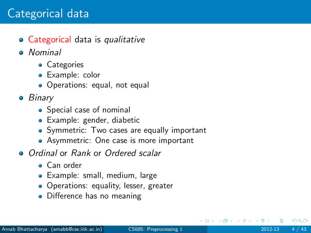
4. Categorical data Categorical data is qualitative Nominal Categories Example: color Operations: equal, not equal Binary Special case of nominal Example: gender, diabetic Symmetric: Two cases are equally important Asymmetric: One case is more important Ordinal or Rank or Ordered scalar Can order Example: small, medium, large Operations: equality, lesser, greater Difference has no meaning Arnab Bhattacharya (arnabb@cse.iitk.ac.in) CS685: Preprocessing 1 2012-13 4 / 43
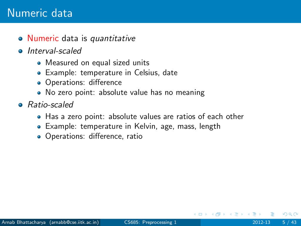
5. Numeric data Numeric data is quantitative Interval-scaled Measured on equal sized units Example: temperature in Celsius, date Operations: difference No zero point: absolute value has no meaning Ratio-scaled Has a zero point: absolute values are ratios of each other Example: temperature in Kelvin, age, mass, length Operations: difference, ratio Arnab Bhattacharya (arnabb@cse.iitk.ac.in) CS685: Preprocessing 1 2012-13 5 / 43
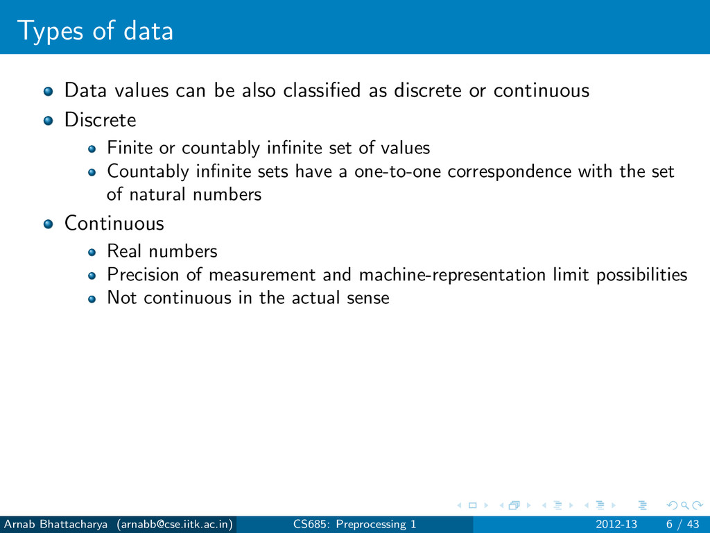
6. Types of data Data values can be also classified as discrete or continuous Discrete Finite or countably infinite set of values Countably infinite sets have a one-to-one correspondence with the set of natural numbers Continuous Real numbers Precision of measurement and machine-representation limit possibilities Not continuous in the actual sense Arnab Bhattacharya (arnabb@cse.iitk.ac.in) CS685: Preprocessing 1 2012-13 6 / 43
7. Data quality Data should have the following qualities Accuracy Completeness Consistency Timeliness Reliability Interpretability Availability Arnab Bhattacharya (arnabb@cse.iitk.ac.in) CS685: Preprocessing 1 2012-13 7 / 43
8. Data quality errors and parameters Errors in data due to Measurement error Data collection error Noise: probabilistic Artifact: deterministic distortions Arnab Bhattacharya (arnabb@cse.iitk.ac.in) CS685: Preprocessing 1 2012-13 8 / 43
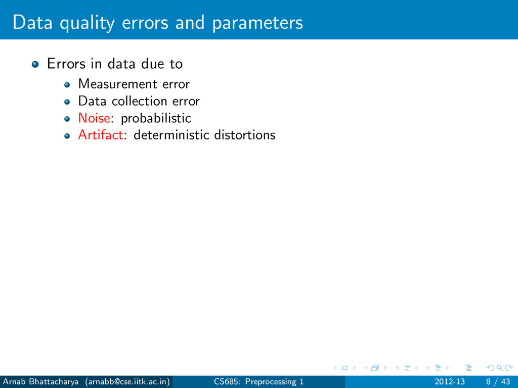
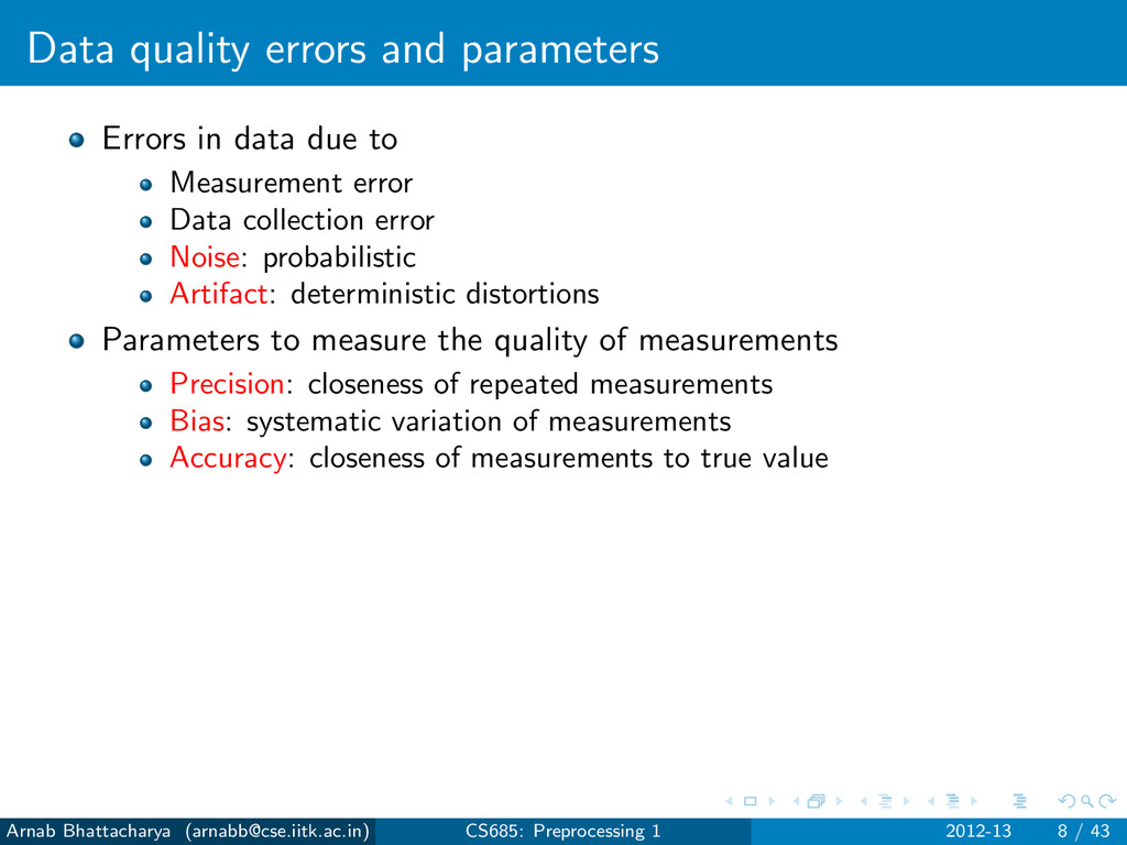
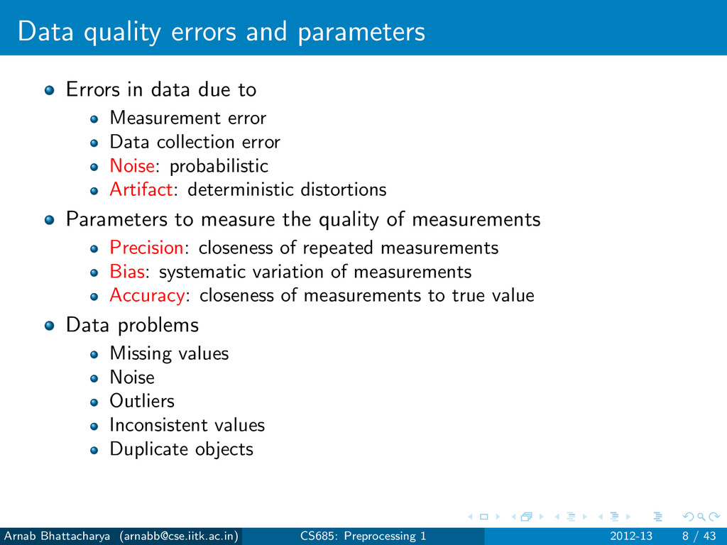
9. Data quality errors and parameters Errors in data due to Measurement error Data collection error Noise: probabilistic Artifact: deterministic distortions Parameters to measure the quality of measurements Precision: closeness of repeated measurements Bias: systematic variation of measurements Accuracy: closeness of measurements to true value Arnab Bhattacharya (arnabb@cse.iitk.ac.in) CS685: Preprocessing 1 2012-13 8 / 43
10. Data quality errors and parameters Errors in data due to Measurement error Data collection error Noise: probabilistic Artifact: deterministic distortions Parameters to measure the quality of measurements Precision: closeness of repeated measurements Bias: systematic variation of measurements Accuracy: closeness of measurements to true value Data problems Missing values Noise Outliers Inconsistent values Duplicate objects Arnab Bhattacharya (arnabb@cse.iitk.ac.in) CS685: Preprocessing 1 2012-13 8 / 43
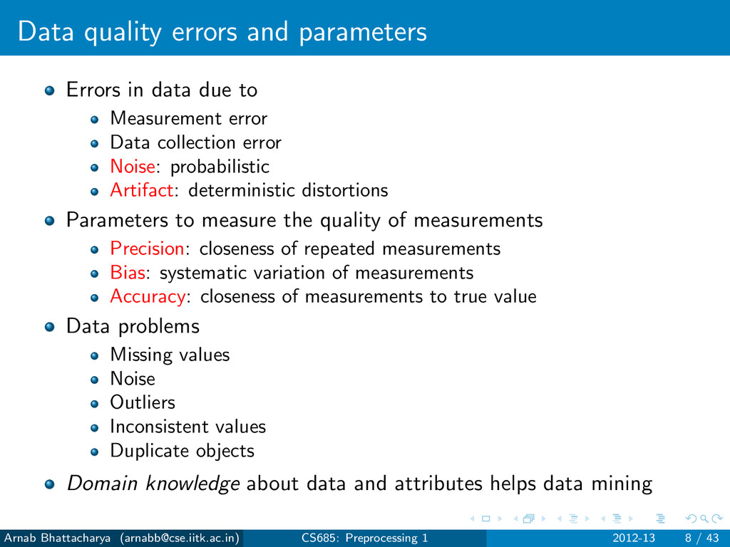
11. Data quality errors and parameters Errors in data due to Measurement error Data collection error Noise: probabilistic Artifact: deterministic distortions Parameters to measure the quality of measurements Precision: closeness of repeated measurements Bias: systematic variation of measurements Accuracy: closeness of measurements to true value Data problems Missing values Noise Outliers Inconsistent values Duplicate objects Domain knowledge about data and attributes helps data mining Arnab Bhattacharya (arnabb@cse.iitk.ac.in) CS685: Preprocessing 1 2012-13 8 / 43
12. Outline 1 Data 2 Data preprocessing 3 Data cleaning 4 Data reduction Dimensionality reduction Numerosity reduction Arnab Bhattacharya (arnabb@cse.iitk.ac.in) CS685: Preprocessing 1 2012-13 9 / 43
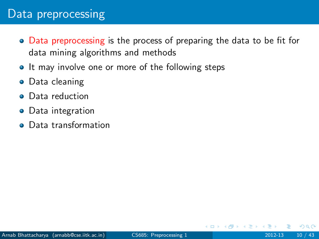
13. Data preprocessing Data preprocessing is the process of preparing the data to be fit for data mining algorithms and methods It may involve one or more of the following steps Data cleaning Data reduction Data integration Data transformation Arnab Bhattacharya (arnabb@cse.iitk.ac.in) CS685: Preprocessing 1 2012-13 10 / 43
14. Outline 1 Data 2 Data preprocessing 3 Data cleaning 4 Data reduction Dimensionality reduction Numerosity reduction Arnab Bhattacharya (arnabb@cse.iitk.ac.in) CS685: Preprocessing 1 2012-13 11 / 43
15. Data cleaning Process of handling errors in data Five major ways Filling in missing values Handling noise Removing outliers One of the main methods in handling noise Resolving inconsistent data Out of range Once identified as inconsistent data, handled as missing value De-duplicating duplicated objects Arnab Bhattacharya (arnabb@cse.iitk.ac.in) CS685: Preprocessing 1 2012-13 12 / 43
16. Missing values Ignore the data object Ignore only the missing attribute during analysis Estimate the missing value Arnab Bhattacharya (arnabb@cse.iitk.ac.in) CS685: Preprocessing 1 2012-13 13 / 43
17. Missing values Ignore the data object Ignore only the missing attribute during analysis Estimate the missing value Use a measure of overall central tendency Mean or median Use a measure of central tendency from only the neighborhood Interpolation Useful for temporal and spatial data Use the most probable value Mode Arnab Bhattacharya (arnabb@cse.iitk.ac.in) CS685: Preprocessing 1 2012-13 13 / 43
18. Noise Random perturbations in the data It is generally assumed that magnitude of noise is smaller than magnitude of attribute of interest Signal-to-noise ratio should not be too low White noise Gaussian distribution with zero mean Arnab Bhattacharya (arnabb@cse.iitk.ac.in) CS685: Preprocessing 1 2012-13 14 / 43
19. Noise Random perturbations in the data It is generally assumed that magnitude of noise is smaller than magnitude of attribute of interest Signal-to-noise ratio should not be too low White noise Gaussian distribution with zero mean Histogram binning Bin values are replaced by mean or median Equi-width histograms are more common than equi-depth Regression Fitting a function to describe the values Small values of noise do not affect the overall fit Noisy value replaced by most likely value predicted by the function Outlier identification and removal Arnab Bhattacharya (arnabb@cse.iitk.ac.in) CS685: Preprocessing 1 2012-13 14 / 43
20. Noise Random perturbations in the data It is generally assumed that magnitude of noise is smaller than magnitude of attribute of interest Signal-to-noise ratio should not be too low White noise Gaussian distribution with zero mean Histogram binning Bin values are replaced by mean or median Equi-width histograms are more common than equi-depth Regression Fitting a function to describe the values Small values of noise do not affect the overall fit Noisy value replaced by most likely value predicted by the function Outlier identification and removal As opposed to noise, bias can be corrected since it is deterministic Arnab Bhattacharya (arnabb@cse.iitk.ac.in) CS685: Preprocessing 1 2012-13 14 / 43
21. Outliers Outliers are data objects that are generated from a perceivably different process Values are considerably unusual Also called anomalous It is not straightforward to identify outliers Unusual values may be the one that are of interest Statistical methods and tests are mostly used Arnab Bhattacharya (arnabb@cse.iitk.ac.in) CS685: Preprocessing 1 2012-13 15 / 43
22. Data duplication Duplicate objects may appear during data insertion or data transfer Introduces errors in statistics about the data If most attributes are exact copies, then it is easy to remove Sometimes one or more attributes are slightly different Domain knowledge needs to be utilized to identify such cases Arnab Bhattacharya (arnabb@cse.iitk.ac.in) CS685: Preprocessing 1 2012-13 16 / 43
23. Outline 1 Data 2 Data preprocessing 3 Data cleaning 4 Data reduction Dimensionality reduction Numerosity reduction Arnab Bhattacharya (arnabb@cse.iitk.ac.in) CS685: Preprocessing 1 2012-13 17 / 43
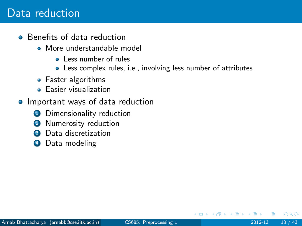
24. Data reduction Benefits of data reduction More understandable model Less number of rules Less complex rules, i.e., involving less number of attributes Faster algorithms Easier visualization Important ways of data reduction 1 Dimensionality reduction 2 Numerosity reduction 3 Data discretization 4 Data modeling Arnab Bhattacharya (arnabb@cse.iitk.ac.in) CS685: Preprocessing 1 2012-13 18 / 43
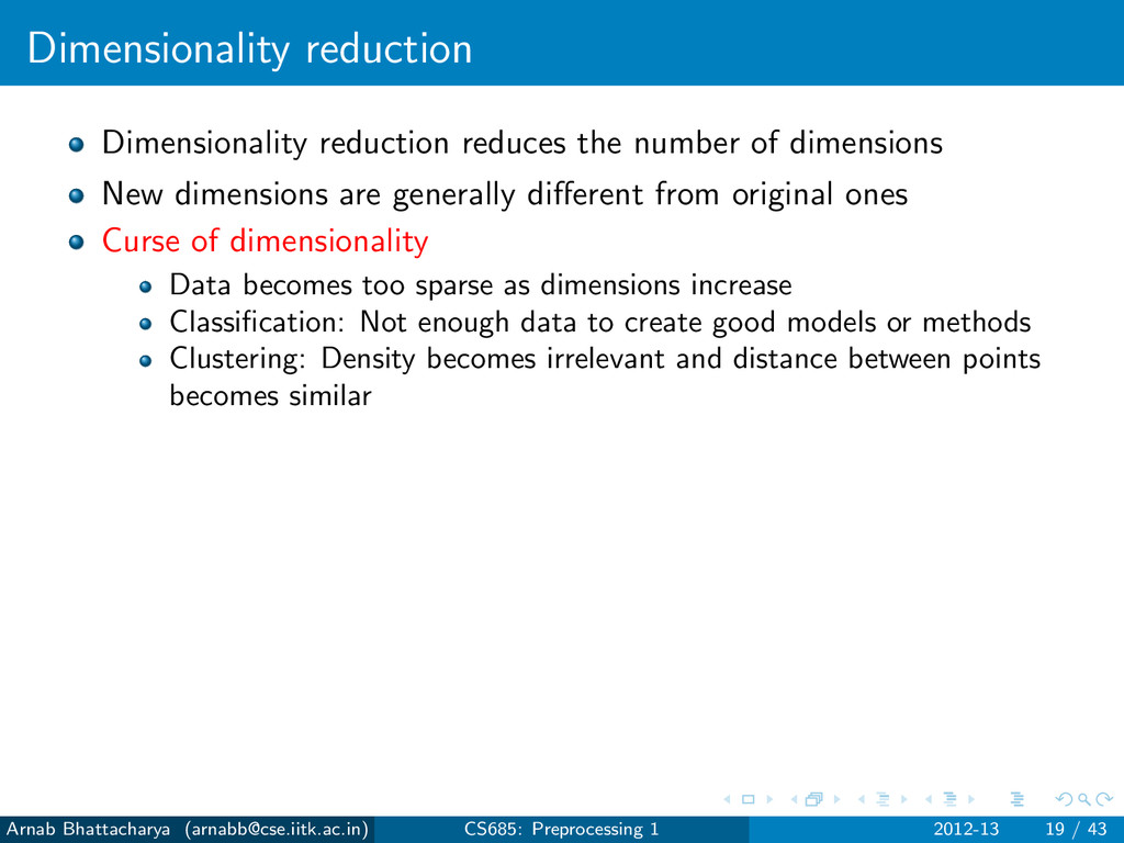
25. Dimensionality reduction Dimensionality reduction reduces the number of dimensions New dimensions are generally different from original ones Curse of dimensionality Data becomes too sparse as dimensions increase Classification: Not enough data to create good models or methods Clustering: Density becomes irrelevant and distance between points becomes similar Arnab Bhattacharya (arnabb@cse.iitk.ac.in) CS685: Preprocessing 1 2012-13 19 / 43
26. Singular value decomposition (SVD) Factorization of a matrix A = UΣV T If A is of size m × n, then U is m × m, V is n × n and Σ is m × n matrix Columns of U are eigenvectors of AAT Left singular vectors UUT = Im (orthonormal) Columns of V are eigenvectors of AT A Right singular vectors V T V = In (orthonormal) σii are the singular values Σ is diagonal Singular values are positive square roots of eigenvalues of AAT or AT A σ11 ≥ σ22 ≥ · · · ≥ σnn (assuming n singular values) Arnab Bhattacharya (arnabb@cse.iitk.ac.in) CS685: Preprocessing 1 2012-13 20 / 43
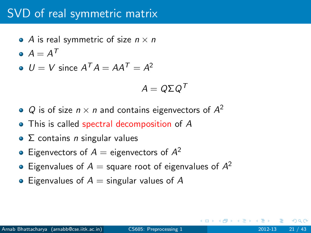
27. SVD of real symmetric matrix A is real symmetric of size n × n A = AT U = V since AT A = AAT = A2 A = QΣQT Q is of size n × n and contains eigenvectors of A2 This is called spectral decomposition of A Σ contains n singular values Eigenvectors of A = eigenvectors of A2 Eigenvalues of A = square root of eigenvalues of A2 Eigenvalues of A = singular values of A Arnab Bhattacharya (arnabb@cse.iitk.ac.in) CS685: Preprocessing 1 2012-13 21 / 43
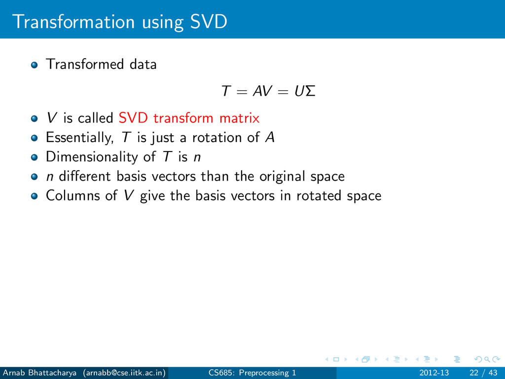
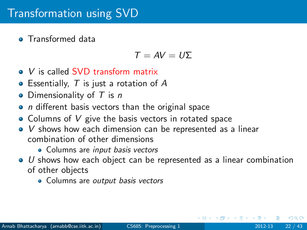
28. Transformation using SVD Transformed data T = AV = UΣ V is called SVD transform matrix Essentially, T is just a rotation of A Dimensionality of T is n n different basis vectors than the original space Columns of V give the basis vectors in rotated space Arnab Bhattacharya (arnabb@cse.iitk.ac.in) CS685: Preprocessing 1 2012-13 22 / 43
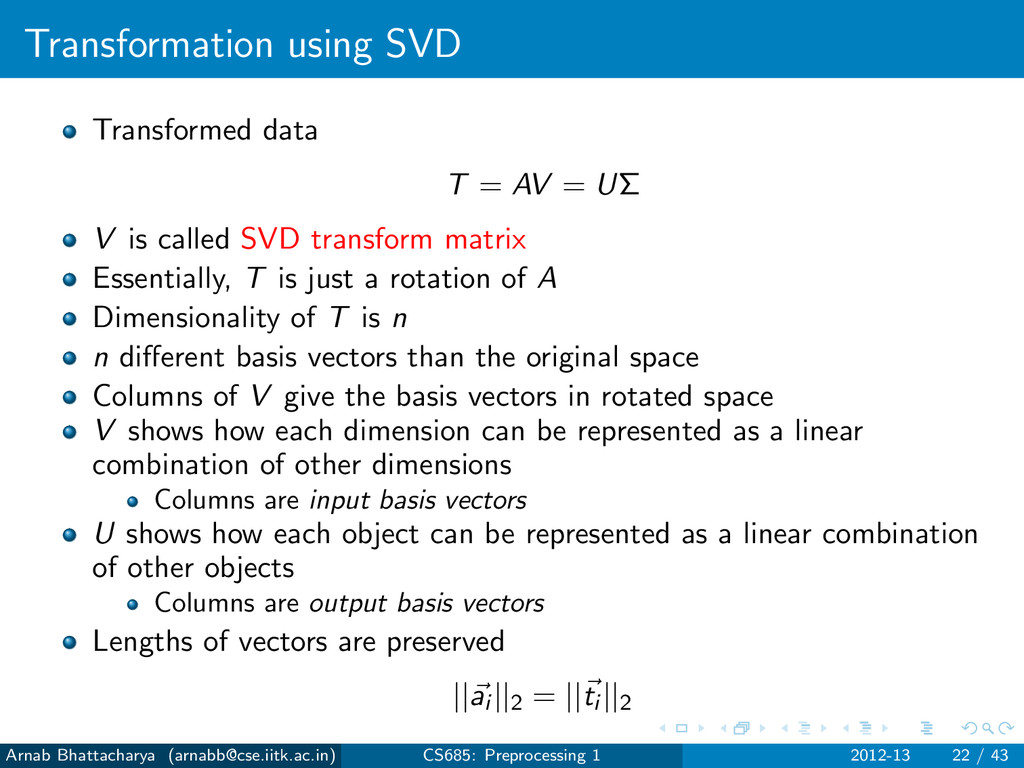
29. Transformation using SVD Transformed data T = AV = UΣ V is called SVD transform matrix Essentially, T is just a rotation of A Dimensionality of T is n n different basis vectors than the original space Columns of V give the basis vectors in rotated space V shows how each dimension can be represented as a linear combination of other dimensions Columns are input basis vectors U shows how each object can be represented as a linear combination of other objects Columns are output basis vectors Arnab Bhattacharya (arnabb@cse.iitk.ac.in) CS685: Preprocessing 1 2012-13 22 / 43
30. Transformation using SVD Transformed data T = AV = UΣ V is called SVD transform matrix Essentially, T is just a rotation of A Dimensionality of T is n n different basis vectors than the original space Columns of V give the basis vectors in rotated space V shows how each dimension can be represented as a linear combination of other dimensions Columns are input basis vectors U shows how each object can be represented as a linear combination of other objects Columns are output basis vectors Lengths of vectors are preserved ||ai ||2 = ||ti ||2 Arnab Bhattacharya (arnabb@cse.iitk.ac.in) CS685: Preprocessing 1 2012-13 22 / 43
31. Example A     2 4 1 3 0 1 −1 0.5     =U     −0.80 0.22 0.05 0.54 −0.56 −0.20 −0.34 −0.71 −0.16 −0.31 0.90 −0.21 −0.01 −0.89 −0.22 0.37     × Σ     5.54 0 0 1.24 0 0 0 0     × V T −0.39 −0.92 0.92 −0.39 T T = AV = UΣ =     2 4 1 3 0 1 −1 0.5     × −0.39 −0.92 0.92 −0.39 =     −4.46 0.27 −3.15 −0.25 −0.92 −0.39 −0.06 −1.15     Arnab Bhattacharya (arnabb@cse.iitk.ac.in) CS685: Preprocessing 1 2012-13 23 / 43
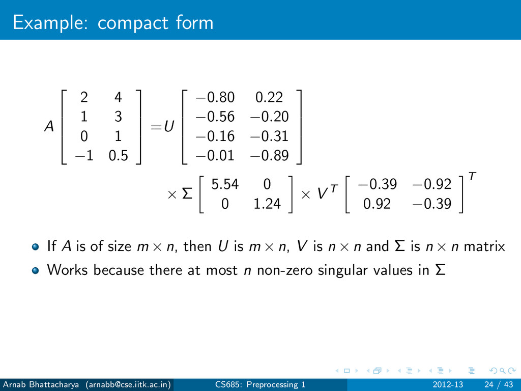
32. Example: compact form A     2 4 1 3 0 1 −1 0.5     =U     −0.80 0.22 −0.56 −0.20 −0.16 −0.31 −0.01 −0.89     × Σ 5.54 0 0 1.24 × V T −0.39 −0.92 0.92 −0.39 T If A is of size m × n, then U is m × n, V is n × n and Σ is n × n matrix Works because there at most n non-zero singular values in Σ Arnab Bhattacharya (arnabb@cse.iitk.ac.in) CS685: Preprocessing 1 2012-13 24 / 43
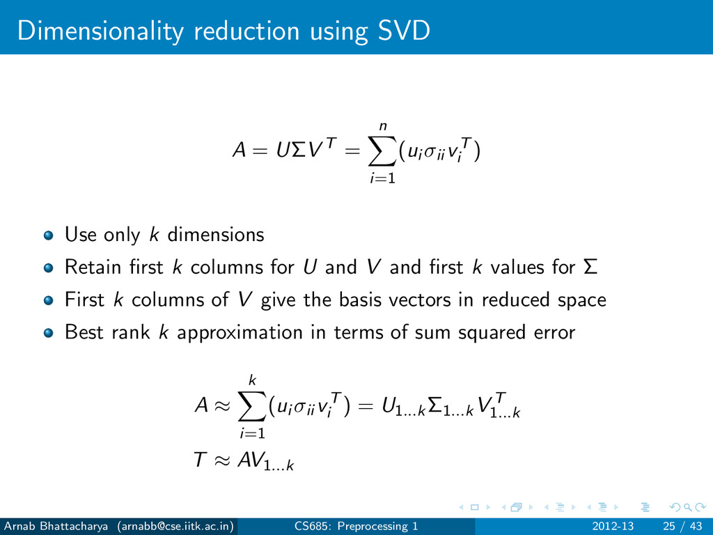
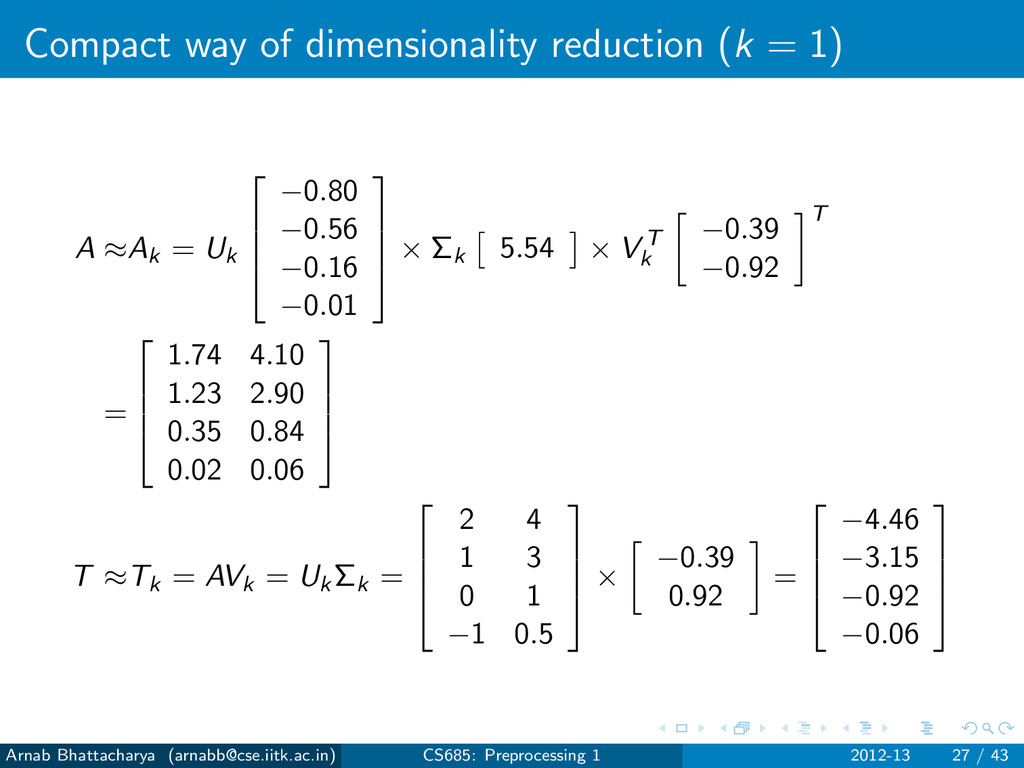
33. Dimensionality reduction using SVD A = UΣV T = n i=1 (ui σii vT i ) Use only k dimensions Retain first k columns for U and V and first k values for Σ First k columns of V give the basis vectors in reduced space Best rank k approximation in terms of sum squared error A ≈ k i=1 (ui σii vT i ) = U1...kΣ1...kV T 1...k T ≈ AV1...k Arnab Bhattacharya (arnabb@cse.iitk.ac.in) CS685: Preprocessing 1 2012-13 25 / 43
34. Example of dimensionality reduction (k = 1) A ≈Ak = Uk     −0.80 0 0 0 −0.56 0 0 0 −0.16 0 0 0 −0.01 0 0 0     × Σk     5.54 0 0 0 0 0 0 0     × V T k −0.39 0 −0.92 0 T =     1.74 4.10 1.23 2.90 0.35 0.84 0.02 0.06     T ≈Tk = AVk = UkΣk =     2 4 1 3 0 1 −1 0.5     × −0.39 0 0.92 0 =     −4.46 0 −3.15 0 −0.92 0 −0.06 0     Arnab Bhattacharya (arnabb@cse.iitk.ac.in) CS685: Preprocessing 1 2012-13 26 / 43
35. Compact way of dimensionality reduction (k = 1) A ≈Ak = Uk     −0.80 −0.56 −0.16 −0.01     × Σk 5.54 × V T k −0.39 −0.92 T =     1.74 4.10 1.23 2.90 0.35 0.84 0.02 0.06     T ≈Tk = AVk = UkΣk =     2 4 1 3 0 1 −1 0.5     × −0.39 0.92 =     −4.46 −3.15 −0.92 −0.06     Arnab Bhattacharya (arnabb@cse.iitk.ac.in) CS685: Preprocessing 1 2012-13 27 / 43
36. How many dimensions to retain? Arnab Bhattacharya (arnabb@cse.iitk.ac.in) CS685: Preprocessing 1 2012-13 28 / 43
37. How many dimensions to retain? There is no easy answer Arnab Bhattacharya (arnabb@cse.iitk.ac.in) CS685: Preprocessing 1 2012-13 28 / 43
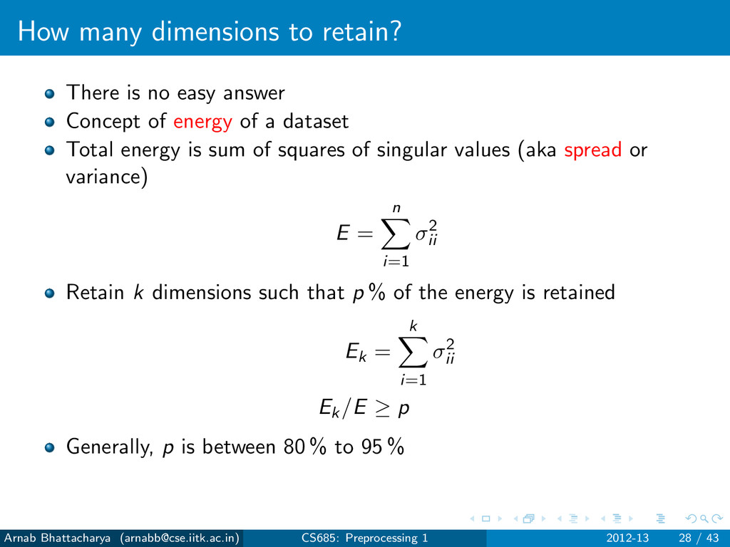
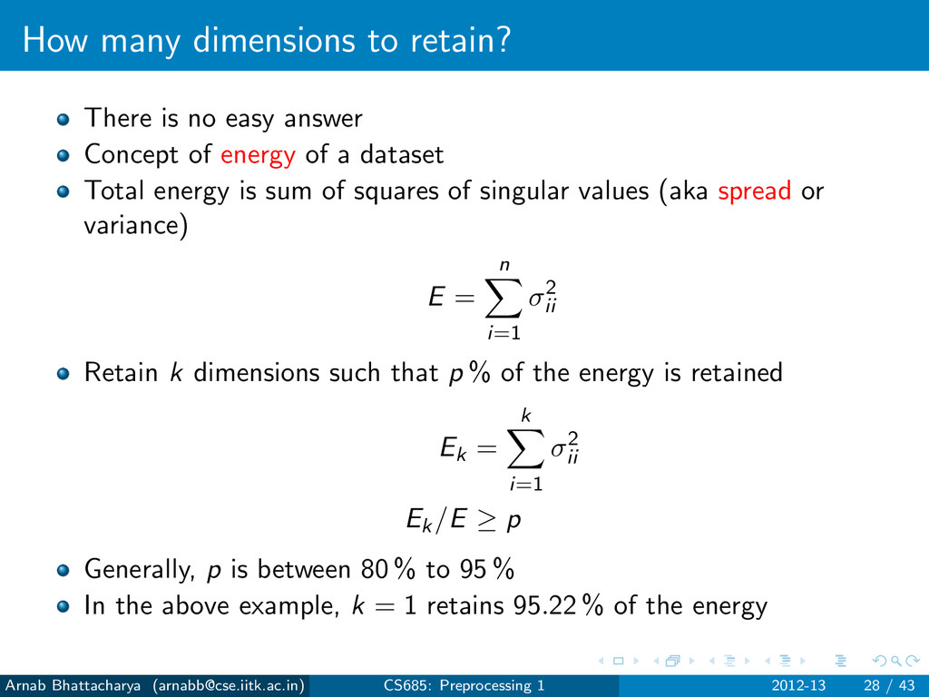
38. How many dimensions to retain? There is no easy answer Concept of energy of a dataset Total energy is sum of squares of singular values (aka spread or variance) E = n i=1 σ2 ii Retain k dimensions such that p % of the energy is retained Ek = k i=1 σ2 ii Ek/E ≥ p Generally, p is between 80 % to 95 % Arnab Bhattacharya (arnabb@cse.iitk.ac.in) CS685: Preprocessing 1 2012-13 28 / 43
39. How many dimensions to retain? There is no easy answer Concept of energy of a dataset Total energy is sum of squares of singular values (aka spread or variance) E = n i=1 σ2 ii Retain k dimensions such that p % of the energy is retained Ek = k i=1 σ2 ii Ek/E ≥ p Generally, p is between 80 % to 95 % In the above example, k = 1 retains 95.22 % of the energy Arnab Bhattacharya (arnabb@cse.iitk.ac.in) CS685: Preprocessing 1 2012-13 28 / 43
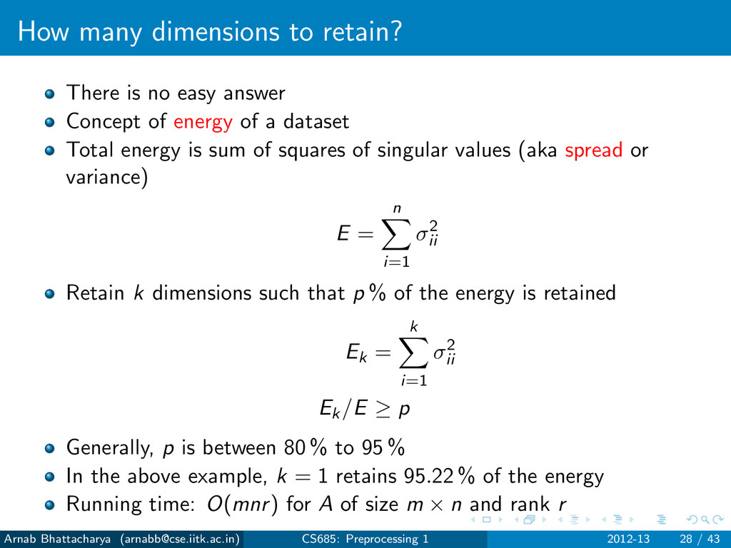
40. How many dimensions to retain? There is no easy answer Concept of energy of a dataset Total energy is sum of squares of singular values (aka spread or variance) E = n i=1 σ2 ii Retain k dimensions such that p % of the energy is retained Ek = k i=1 σ2 ii Ek/E ≥ p Generally, p is between 80 % to 95 % In the above example, k = 1 retains 95.22 % of the energy Running time: O(mnr) for A of size m × n and rank r Arnab Bhattacharya (arnabb@cse.iitk.ac.in) CS685: Preprocessing 1 2012-13 28 / 43
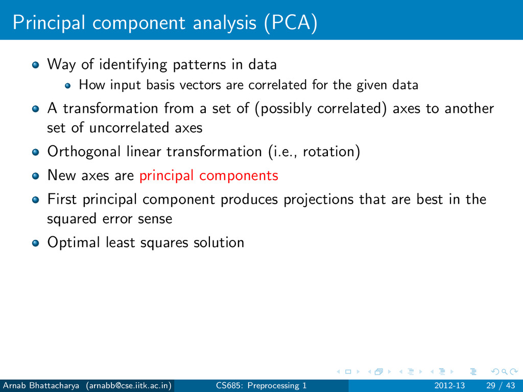
41. Principal component analysis (PCA) Way of identifying patterns in data How input basis vectors are correlated for the given data A transformation from a set of (possibly correlated) axes to another set of uncorrelated axes Orthogonal linear transformation (i.e., rotation) New axes are principal components First principal component produces projections that are best in the squared error sense Optimal least squares solution Arnab Bhattacharya (arnabb@cse.iitk.ac.in) CS685: Preprocessing 1 2012-13 29 / 43
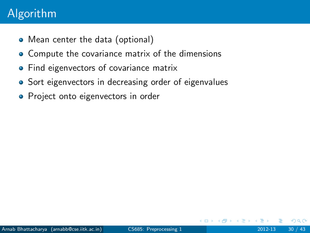
42. Algorithm Mean center the data (optional) Compute the covariance matrix of the dimensions Find eigenvectors of covariance matrix Sort eigenvectors in decreasing order of eigenvalues Project onto eigenvectors in order Arnab Bhattacharya (arnabb@cse.iitk.ac.in) CS685: Preprocessing 1 2012-13 30 / 43
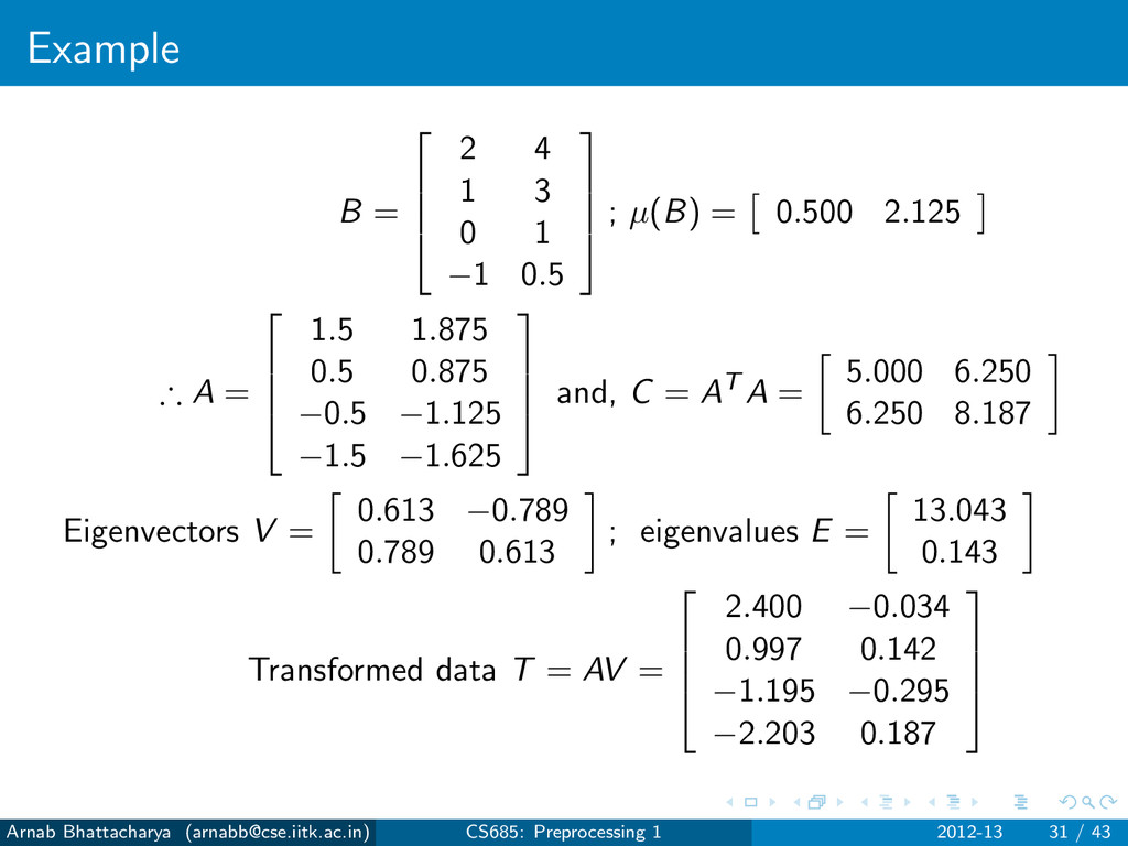
43. Algorithm Mean center the data (optional) Compute the covariance matrix of the dimensions Find eigenvectors of covariance matrix Sort eigenvectors in decreasing order of eigenvalues Project onto eigenvectors in order Assume data matrix is B of size m × n For each dimension, compute mean µi Mean center B by subtracting µi from each column i to get A Compute covariance matrix C of size n × n If mean centered, C = AT A Find eigenvectors and corresponding eigenvalues (V , E) of C Sort eigenvalues such that e1 ≥ e2 ≥ · · · ≥ en Project step-by-step onto the principal components v1, v2, . . . , etc. Arnab Bhattacharya (arnabb@cse.iitk.ac.in) CS685: Preprocessing 1 2012-13 30 / 43
44. Example B =     2 4 1 3 0 1 −1 0.5     ; µ(B) = 0.500 2.125 ∴ A =     1.5 1.875 0.5 0.875 −0.5 −1.125 −1.5 −1.625     and, C = AT A = 5.000 6.250 6.250 8.187 Eigenvectors V = 0.613 −0.789 0.789 0.613 ; eigenvalues E = 13.043 0.143 Transformed data T = AV =     2.400 −0.034 0.997 0.142 −1.195 −0.295 −2.203 0.187     Arnab Bhattacharya (arnabb@cse.iitk.ac.in) CS685: Preprocessing 1 2012-13 31 / 43
45. Visual example Arnab Bhattacharya (arnabb@cse.iitk.ac.in) CS685: Preprocessing 1 2012-13 32 / 43
46. Properties Also known as Karhunen-Lo` eve transform (KLT) Arnab Bhattacharya (arnabb@cse.iitk.ac.in) CS685: Preprocessing 1 2012-13 33 / 43
47. Properties Also known as Karhunen-Lo` eve transform (KLT) Works for L2 distances only as others are not invariant to rotation Arnab Bhattacharya (arnabb@cse.iitk.ac.in) CS685: Preprocessing 1 2012-13 33 / 43
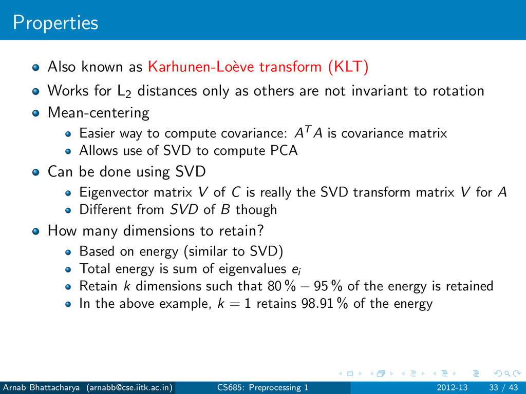
48. Properties Also known as Karhunen-Lo` eve transform (KLT) Works for L2 distances only as others are not invariant to rotation Mean-centering Easier way to compute covariance: AT A is covariance matrix Allows use of SVD to compute PCA Arnab Bhattacharya (arnabb@cse.iitk.ac.in) CS685: Preprocessing 1 2012-13 33 / 43
49. Properties Also known as Karhunen-Lo` eve transform (KLT) Works for L2 distances only as others are not invariant to rotation Mean-centering Easier way to compute covariance: AT A is covariance matrix Allows use of SVD to compute PCA Can be done using SVD Eigenvector matrix V of C is really the SVD transform matrix V for A Different from SVD of B though Arnab Bhattacharya (arnabb@cse.iitk.ac.in) CS685: Preprocessing 1 2012-13 33 / 43
50. Properties Also known as Karhunen-Lo` eve transform (KLT) Works for L2 distances only as others are not invariant to rotation Mean-centering Easier way to compute covariance: AT A is covariance matrix Allows use of SVD to compute PCA Can be done using SVD Eigenvector matrix V of C is really the SVD transform matrix V for A Different from SVD of B though How many dimensions to retain? Based on energy (similar to SVD) Total energy is sum of eigenvalues ei Retain k dimensions such that 80 % − 95 % of the energy is retained Arnab Bhattacharya (arnabb@cse.iitk.ac.in) CS685: Preprocessing 1 2012-13 33 / 43
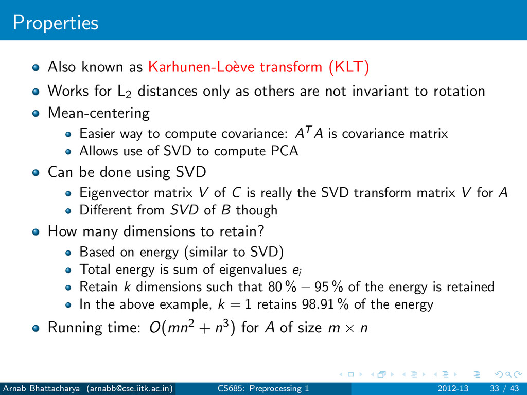
51. Properties Also known as Karhunen-Lo` eve transform (KLT) Works for L2 distances only as others are not invariant to rotation Mean-centering Easier way to compute covariance: AT A is covariance matrix Allows use of SVD to compute PCA Can be done using SVD Eigenvector matrix V of C is really the SVD transform matrix V for A Different from SVD of B though How many dimensions to retain? Based on energy (similar to SVD) Total energy is sum of eigenvalues ei Retain k dimensions such that 80 % − 95 % of the energy is retained In the above example, k = 1 retains 98.91 % of the energy Arnab Bhattacharya (arnabb@cse.iitk.ac.in) CS685: Preprocessing 1 2012-13 33 / 43
52. Properties Also known as Karhunen-Lo` eve transform (KLT) Works for L2 distances only as others are not invariant to rotation Mean-centering Easier way to compute covariance: AT A is covariance matrix Allows use of SVD to compute PCA Can be done using SVD Eigenvector matrix V of C is really the SVD transform matrix V for A Different from SVD of B though How many dimensions to retain? Based on energy (similar to SVD) Total energy is sum of eigenvalues ei Retain k dimensions such that 80 % − 95 % of the energy is retained In the above example, k = 1 retains 98.91 % of the energy Running time: O(mn2 + n3) for A of size m × n Arnab Bhattacharya (arnabb@cse.iitk.ac.in) CS685: Preprocessing 1 2012-13 33 / 43
53. Numerosity reduction Numerosity reduction reduces the volume of data Arnab Bhattacharya (arnabb@cse.iitk.ac.in) CS685: Preprocessing 1 2012-13 34 / 43
54. Numerosity reduction Numerosity reduction reduces the volume of data Reduction in number of data objects Data compression Modeling Discretization Arnab Bhattacharya (arnabb@cse.iitk.ac.in) CS685: Preprocessing 1 2012-13 34 / 43
55. Aggregation Considers a set of data objects having some similar attribute(s) Aggregates some other attribute(s) into single value(s) Example: sum, average Benefits of aggregation Aggregate value has less variability Absorbs individual errors Arnab Bhattacharya (arnabb@cse.iitk.ac.in) CS685: Preprocessing 1 2012-13 35 / 43
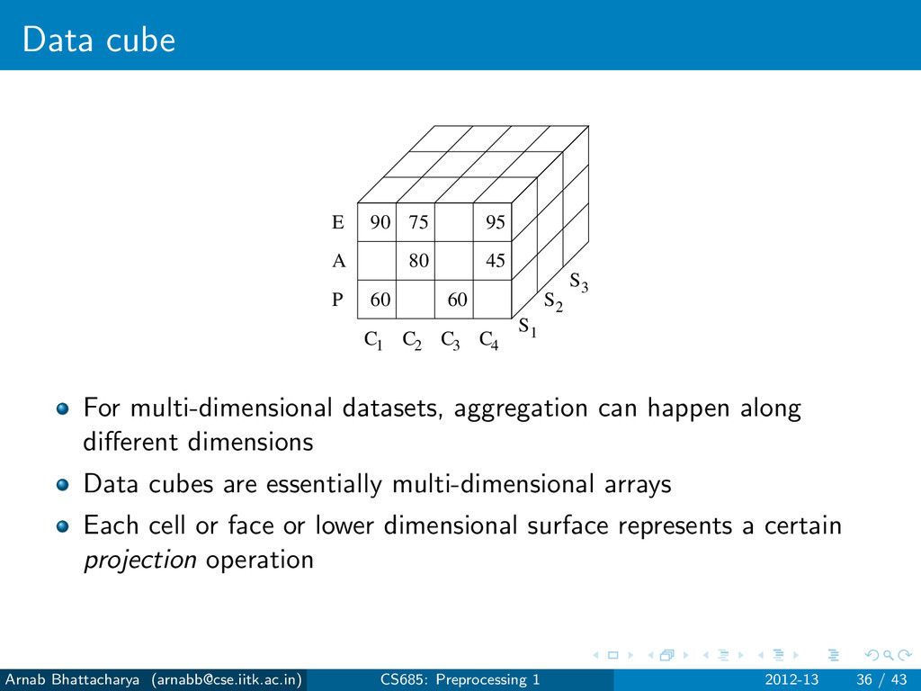
56. Data cube S1 S2 S3 C1 C2 C3 C4 A E P 90 75 80 95 45 60 60 For multi-dimensional datasets, aggregation can happen along different dimensions Data cubes are essentially multi-dimensional arrays Each cell or face or lower dimensional surface represents a certain projection operation Arnab Bhattacharya (arnabb@cse.iitk.ac.in) CS685: Preprocessing 1 2012-13 36 / 43
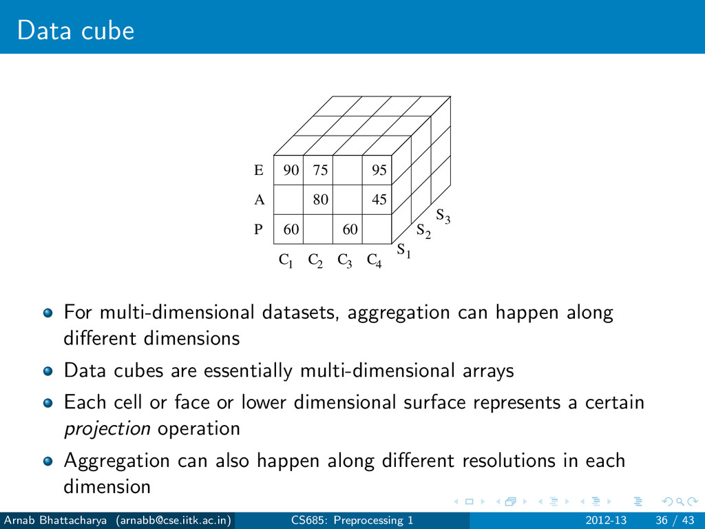
57. Data cube S1 S2 S3 C1 C2 C3 C4 A E P 90 75 80 95 45 60 60 For multi-dimensional datasets, aggregation can happen along different dimensions Data cubes are essentially multi-dimensional arrays Each cell or face or lower dimensional surface represents a certain projection operation Aggregation can also happen along different resolutions in each dimension Arnab Bhattacharya (arnabb@cse.iitk.ac.in) CS685: Preprocessing 1 2012-13 36 / 43
58. Sampling A sample is a representative if it has (approximately) the same property of interest as the full dataset Sampling approaches Arnab Bhattacharya (arnabb@cse.iitk.ac.in) CS685: Preprocessing 1 2012-13 37 / 43
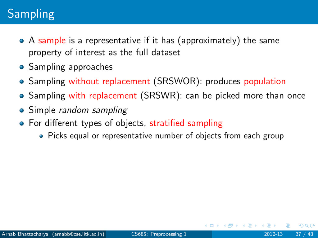
59. Sampling A sample is a representative if it has (approximately) the same property of interest as the full dataset Sampling approaches Sampling without replacement (SRSWOR): produces population Sampling with replacement (SRSWR): can be picked more than once Arnab Bhattacharya (arnabb@cse.iitk.ac.in) CS685: Preprocessing 1 2012-13 37 / 43
60. Sampling A sample is a representative if it has (approximately) the same property of interest as the full dataset Sampling approaches Sampling without replacement (SRSWOR): produces population Sampling with replacement (SRSWR): can be picked more than once Simple random sampling For different types of objects, stratified sampling Picks equal or representative number of objects from each group Arnab Bhattacharya (arnabb@cse.iitk.ac.in) CS685: Preprocessing 1 2012-13 37 / 43
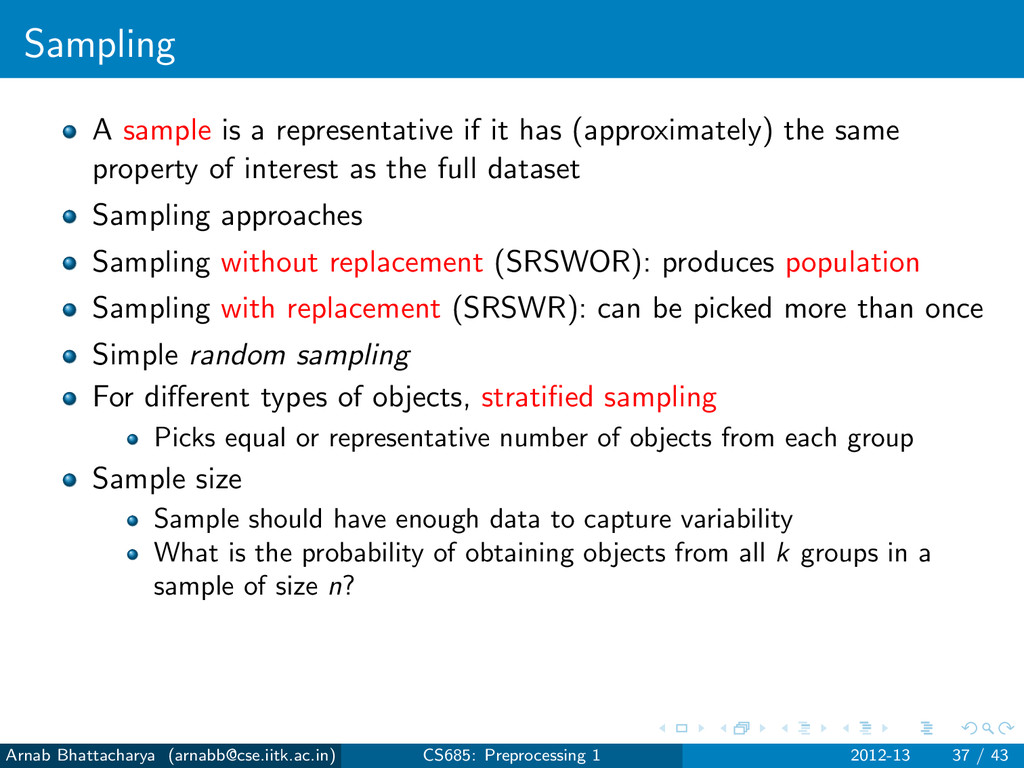
61. Sampling A sample is a representative if it has (approximately) the same property of interest as the full dataset Sampling approaches Sampling without replacement (SRSWOR): produces population Sampling with replacement (SRSWR): can be picked more than once Simple random sampling For different types of objects, stratified sampling Picks equal or representative number of objects from each group Sample size Sample should have enough data to capture variability What is the probability of obtaining objects from all k groups in a sample of size n? Arnab Bhattacharya (arnabb@cse.iitk.ac.in) CS685: Preprocessing 1 2012-13 37 / 43
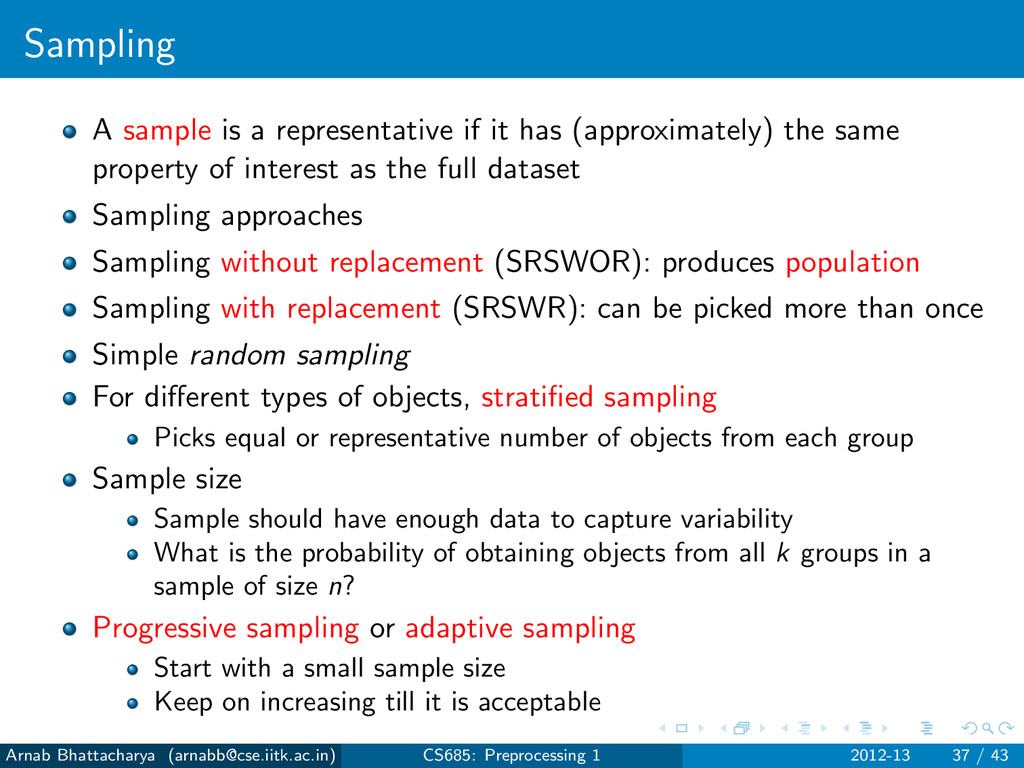
62. Sampling A sample is a representative if it has (approximately) the same property of interest as the full dataset Sampling approaches Sampling without replacement (SRSWOR): produces population Sampling with replacement (SRSWR): can be picked more than once Simple random sampling For different types of objects, stratified sampling Picks equal or representative number of objects from each group Sample size Sample should have enough data to capture variability What is the probability of obtaining objects from all k groups in a sample of size n? Progressive sampling or adaptive sampling Start with a small sample size Keep on increasing till it is acceptable Arnab Bhattacharya (arnabb@cse.iitk.ac.in) CS685: Preprocessing 1 2012-13 37 / 43
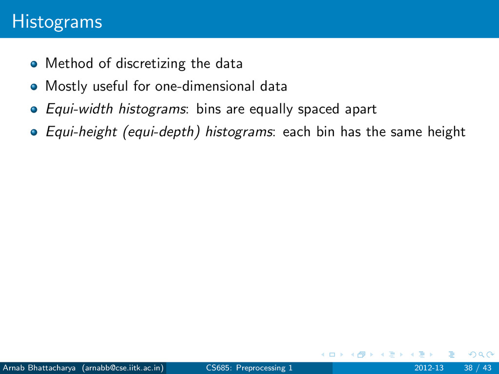
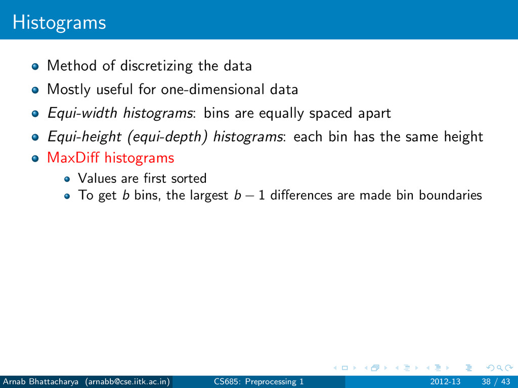
63. Histograms Method of discretizing the data Mostly useful for one-dimensional data Equi-width histograms: bins are equally spaced apart Equi-height (equi-depth) histograms: each bin has the same height Arnab Bhattacharya (arnabb@cse.iitk.ac.in) CS685: Preprocessing 1 2012-13 38 / 43
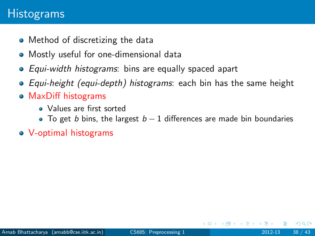
64. Histograms Method of discretizing the data Mostly useful for one-dimensional data Equi-width histograms: bins are equally spaced apart Equi-height (equi-depth) histograms: each bin has the same height MaxDiff histograms Values are first sorted To get b bins, the largest b − 1 differences are made bin boundaries Arnab Bhattacharya (arnabb@cse.iitk.ac.in) CS685: Preprocessing 1 2012-13 38 / 43
65. Histograms Method of discretizing the data Mostly useful for one-dimensional data Equi-width histograms: bins are equally spaced apart Equi-height (equi-depth) histograms: each bin has the same height MaxDiff histograms Values are first sorted To get b bins, the largest b − 1 differences are made bin boundaries V-optimal histograms Arnab Bhattacharya (arnabb@cse.iitk.ac.in) CS685: Preprocessing 1 2012-13 38 / 43
66. V-optimal histograms A dataset with n objects Reduce n to b bins where b n Arnab Bhattacharya (arnabb@cse.iitk.ac.in) CS685: Preprocessing 1 2012-13 39 / 43
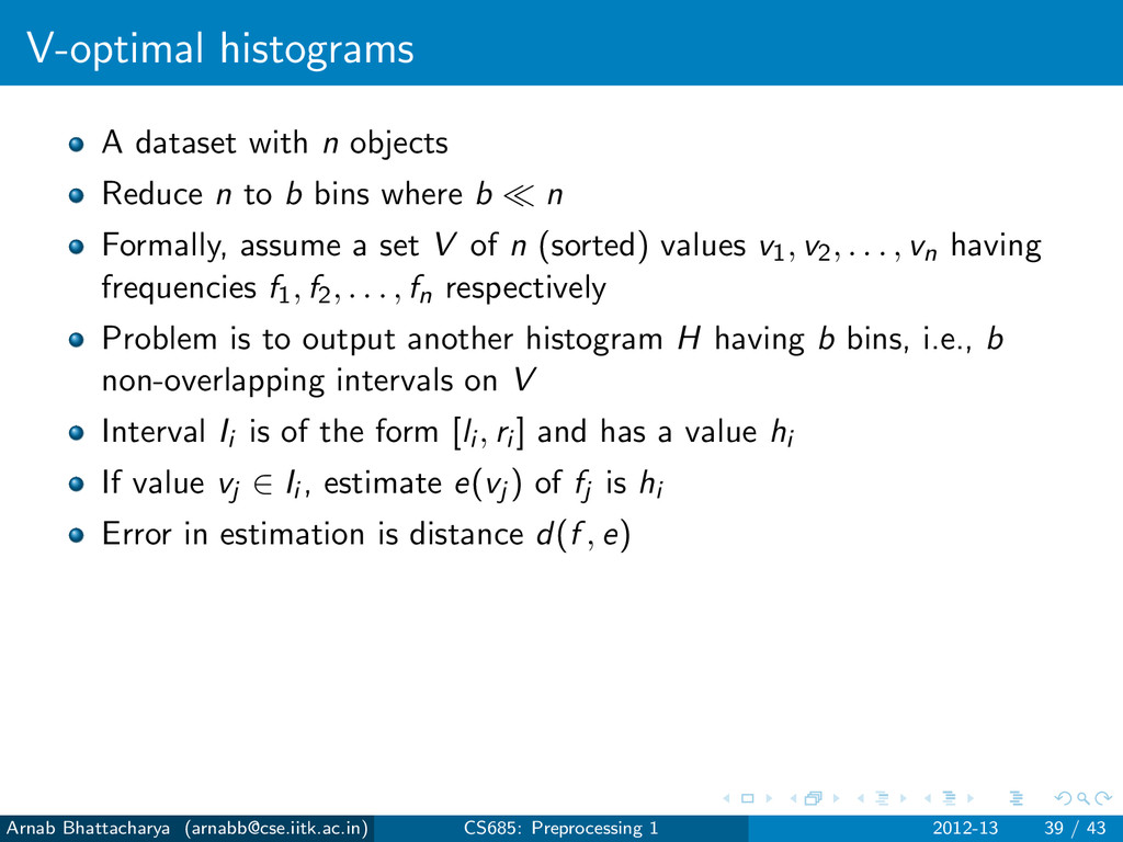
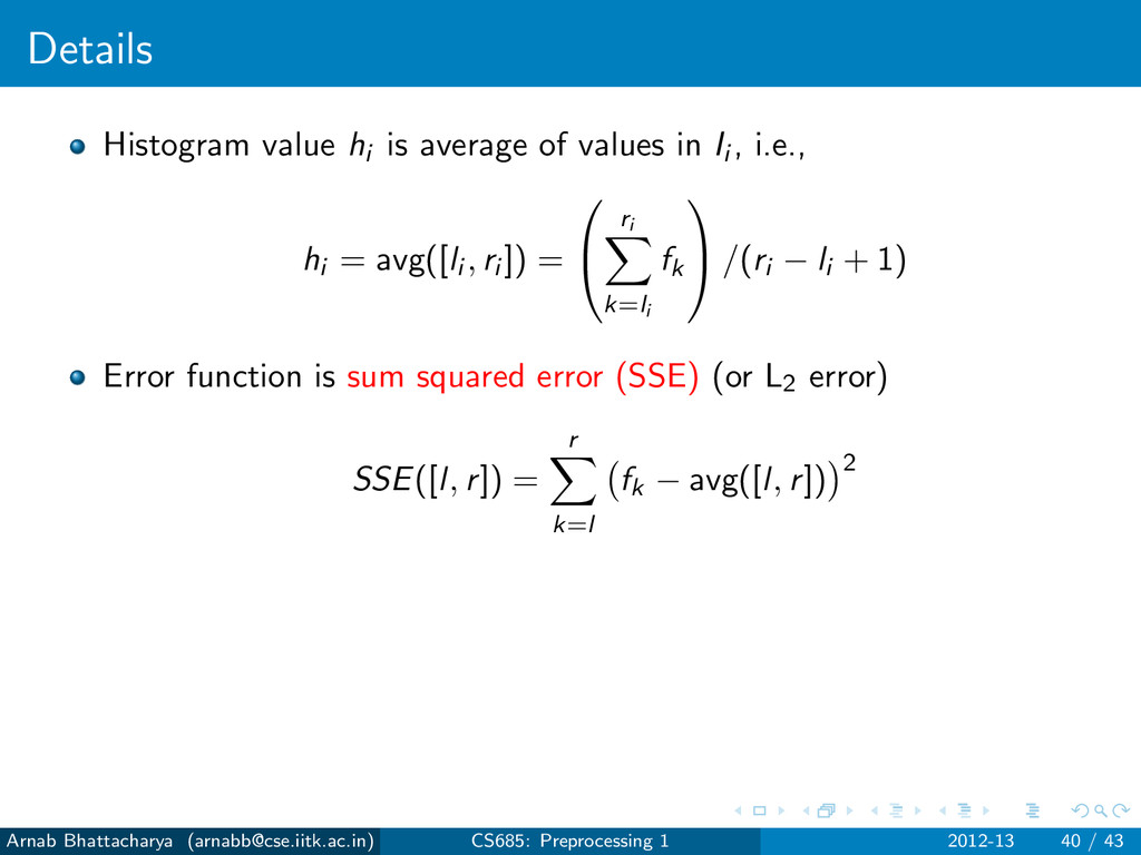
67. V-optimal histograms A dataset with n objects Reduce n to b bins where b n Formally, assume a set V of n (sorted) values v1, v2, . . . , vn having frequencies f1, f2, . . . , fn respectively Problem is to output another histogram H having b bins, i.e., b non-overlapping intervals on V Interval Ii is of the form [li , ri ] and has a value hi If value vj ∈ Ii , estimate e(vj ) of fj is hi Error in estimation is distance d(f , e) Arnab Bhattacharya (arnabb@cse.iitk.ac.in) CS685: Preprocessing 1 2012-13 39 / 43
68. Details Histogram value hi is average of values in Ii , i.e., hi = avg([li , ri ]) =   ri k=li fk   /(ri − li + 1) Error function is sum squared error (SSE) (or L2 error) SSE([l, r]) = r k=l fk − avg([l, r]) 2 Arnab Bhattacharya (arnabb@cse.iitk.ac.in) CS685: Preprocessing 1 2012-13 40 / 43
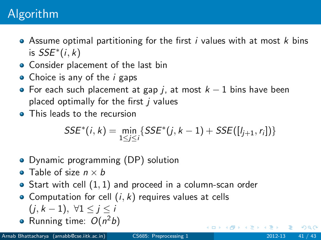
69. Algorithm Assume optimal partitioning for the first i values with at most k bins is SSE∗(i, k) Consider placement of the last bin Choice is any of the i gaps For each such placement at gap j, at most k − 1 bins have been placed optimally for the first j values This leads to the recursion SSE∗(i, k) = min 1≤j≤i {SSE∗(j, k − 1) + SSE([lj+1, ri ])} Arnab Bhattacharya (arnabb@cse.iitk.ac.in) CS685: Preprocessing 1 2012-13 41 / 43
70. Algorithm Assume optimal partitioning for the first i values with at most k bins is SSE∗(i, k) Consider placement of the last bin Choice is any of the i gaps For each such placement at gap j, at most k − 1 bins have been placed optimally for the first j values This leads to the recursion SSE∗(i, k) = min 1≤j≤i {SSE∗(j, k − 1) + SSE([lj+1, ri ])} Dynamic programming (DP) solution Table of size n × b Start with cell (1, 1) and proceed in a column-scan order Computation for cell (i, k) requires values at cells (j, k − 1), ∀1 ≤ j ≤ i Arnab Bhattacharya (arnabb@cse.iitk.ac.in) CS685: Preprocessing 1 2012-13 41 / 43
71. Algorithm Assume optimal partitioning for the first i values with at most k bins is SSE∗(i, k) Consider placement of the last bin Choice is any of the i gaps For each such placement at gap j, at most k − 1 bins have been placed optimally for the first j values This leads to the recursion SSE∗(i, k) = min 1≤j≤i {SSE∗(j, k − 1) + SSE([lj+1, ri ])} Dynamic programming (DP) solution Table of size n × b Start with cell (1, 1) and proceed in a column-scan order Computation for cell (i, k) requires values at cells (j, k − 1), ∀1 ≤ j ≤ i Running time: O(n2b) Arnab Bhattacharya (arnabb@cse.iitk.ac.in) CS685: Preprocessing 1 2012-13 41 / 43
72. Data summarization Central tendency measures Mean: may be weighted Median: “middle” value Mode: dataset may be unimodal or multimodal Midrange: Arnab Bhattacharya (arnabb@cse.iitk.ac.in) CS685: Preprocessing 1 2012-13 42 / 43
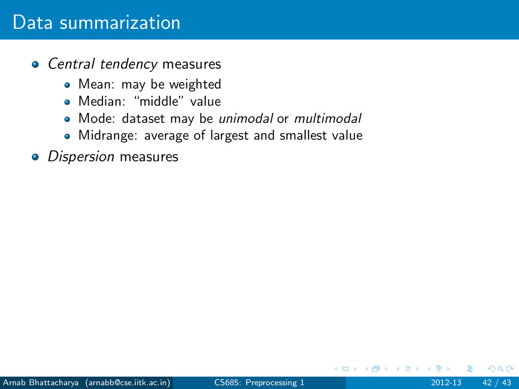
73. Data summarization Central tendency measures Mean: may be weighted Median: “middle” value Mode: dataset may be unimodal or multimodal Midrange: average of largest and smallest value Arnab Bhattacharya (arnabb@cse.iitk.ac.in) CS685: Preprocessing 1 2012-13 42 / 43
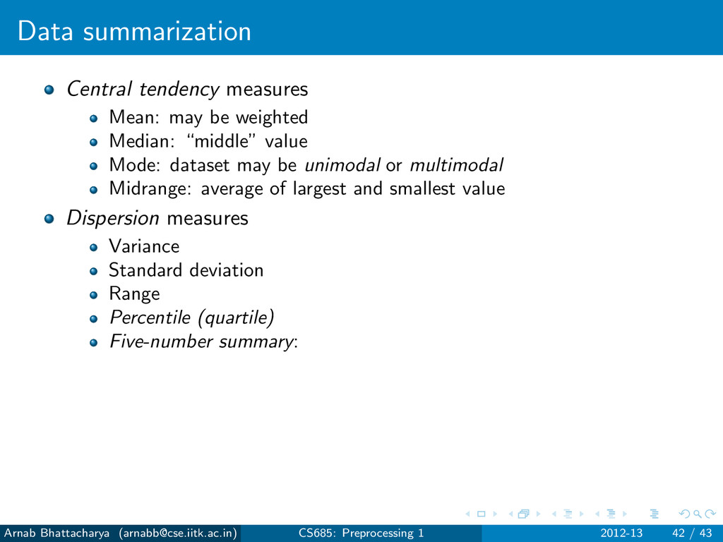
74. Data summarization Central tendency measures Mean: may be weighted Median: “middle” value Mode: dataset may be unimodal or multimodal Midrange: average of largest and smallest value Dispersion measures Arnab Bhattacharya (arnabb@cse.iitk.ac.in) CS685: Preprocessing 1 2012-13 42 / 43
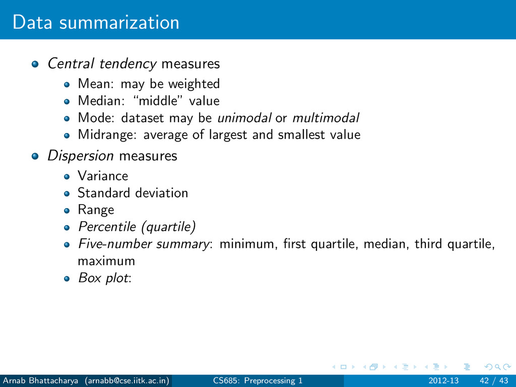
75. Data summarization Central tendency measures Mean: may be weighted Median: “middle” value Mode: dataset may be unimodal or multimodal Midrange: average of largest and smallest value Dispersion measures Variance Standard deviation Range Percentile (quartile) Five-number summary: Arnab Bhattacharya (arnabb@cse.iitk.ac.in) CS685: Preprocessing 1 2012-13 42 / 43
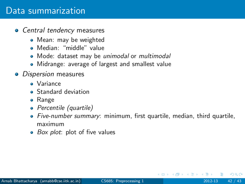
76. Data summarization Central tendency measures Mean: may be weighted Median: “middle” value Mode: dataset may be unimodal or multimodal Midrange: average of largest and smallest value Dispersion measures Variance Standard deviation Range Percentile (quartile) Five-number summary: minimum, first quartile, median, third quartile, maximum Box plot: Arnab Bhattacharya (arnabb@cse.iitk.ac.in) CS685: Preprocessing 1 2012-13 42 / 43
77. Data summarization Central tendency measures Mean: may be weighted Median: “middle” value Mode: dataset may be unimodal or multimodal Midrange: average of largest and smallest value Dispersion measures Variance Standard deviation Range Percentile (quartile) Five-number summary: minimum, first quartile, median, third quartile, maximum Box plot: plot of five values Arnab Bhattacharya (arnabb@cse.iitk.ac.in) CS685: Preprocessing 1 2012-13 42 / 43
78. Data summarization (contd.) Distributive measures Arnab Bhattacharya (arnabb@cse.iitk.ac.in) CS685: Preprocessing 1 2012-13 43 / 43
79. Data summarization (contd.) Distributive measures Can be computed by partitioning the dataset Arnab Bhattacharya (arnabb@cse.iitk.ac.in) CS685: Preprocessing 1 2012-13 43 / 43
80. Data summarization (contd.) Distributive measures Can be computed by partitioning the dataset Example: mean Holistic measures Arnab Bhattacharya (arnabb@cse.iitk.ac.in) CS685: Preprocessing 1 2012-13 43 / 43
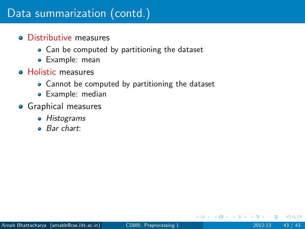
81. Data summarization (contd.) Distributive measures Can be computed by partitioning the dataset Example: mean Holistic measures Cannot be computed by partitioning the dataset Arnab Bhattacharya (arnabb@cse.iitk.ac.in) CS685: Preprocessing 1 2012-13 43 / 43
82. Data summarization (contd.) Distributive measures Can be computed by partitioning the dataset Example: mean Holistic measures Cannot be computed by partitioning the dataset Example: median Arnab Bhattacharya (arnabb@cse.iitk.ac.in) CS685: Preprocessing 1 2012-13 43 / 43
83. Data summarization (contd.) Distributive measures Can be computed by partitioning the dataset Example: mean Holistic measures Cannot be computed by partitioning the dataset Example: median Graphical measures Arnab Bhattacharya (arnabb@cse.iitk.ac.in) CS685: Preprocessing 1 2012-13 43 / 43
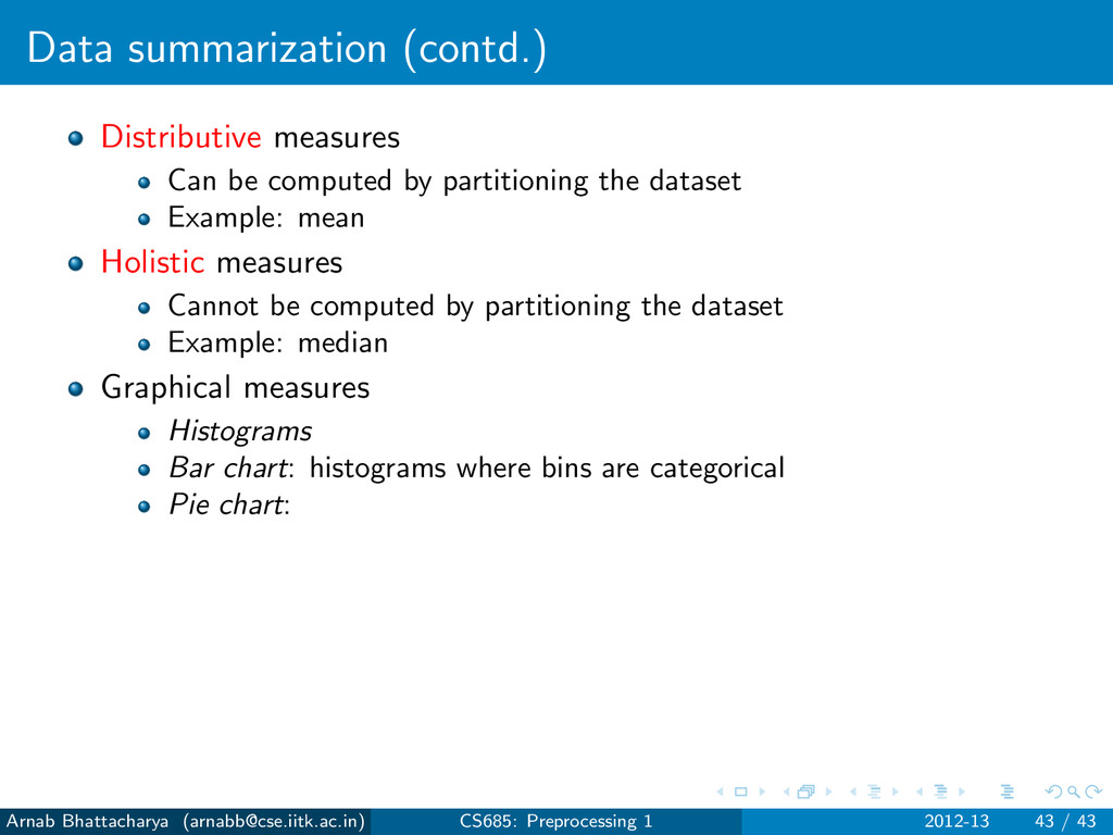
84. Data summarization (contd.) Distributive measures Can be computed by partitioning the dataset Example: mean Holistic measures Cannot be computed by partitioning the dataset Example: median Graphical measures Histograms Bar chart: Arnab Bhattacharya (arnabb@cse.iitk.ac.in) CS685: Preprocessing 1 2012-13 43 / 43
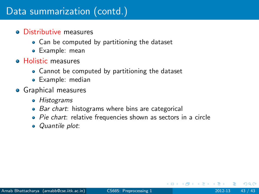
85. Data summarization (contd.) Distributive measures Can be computed by partitioning the dataset Example: mean Holistic measures Cannot be computed by partitioning the dataset Example: median Graphical measures Histograms Bar chart: histograms where bins are categorical Pie chart: Arnab Bhattacharya (arnabb@cse.iitk.ac.in) CS685: Preprocessing 1 2012-13 43 / 43
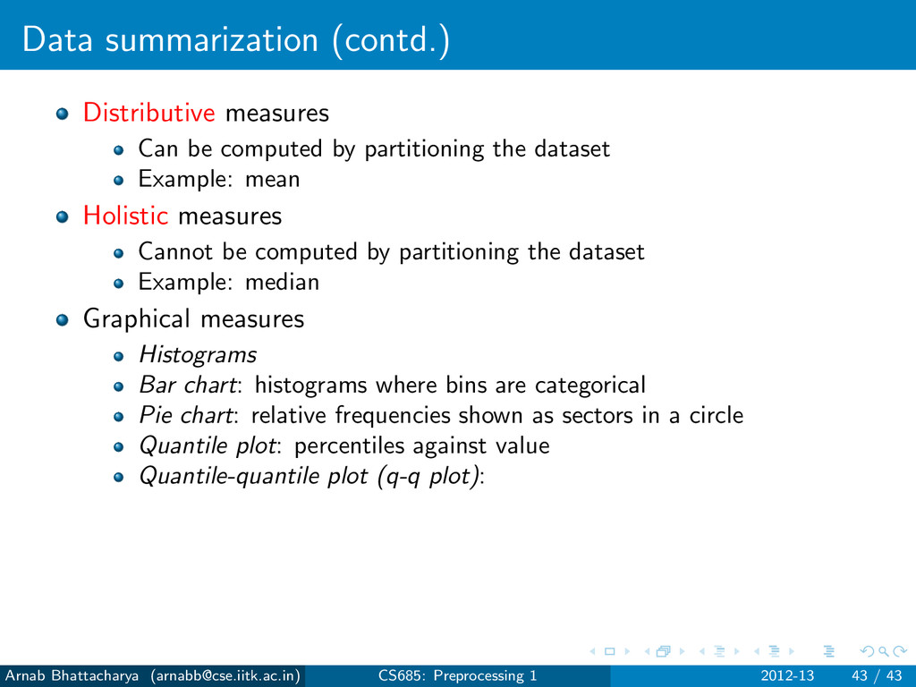
86. Data summarization (contd.) Distributive measures Can be computed by partitioning the dataset Example: mean Holistic measures Cannot be computed by partitioning the dataset Example: median Graphical measures Histograms Bar chart: histograms where bins are categorical Pie chart: relative frequencies shown as sectors in a circle Quantile plot: Arnab Bhattacharya (arnabb@cse.iitk.ac.in) CS685: Preprocessing 1 2012-13 43 / 43
87. Data summarization (contd.) Distributive measures Can be computed by partitioning the dataset Example: mean Holistic measures Cannot be computed by partitioning the dataset Example: median Graphical measures Histograms Bar chart: histograms where bins are categorical Pie chart: relative frequencies shown as sectors in a circle Quantile plot: percentiles against value Quantile-quantile plot (q-q plot): Arnab Bhattacharya (arnabb@cse.iitk.ac.in) CS685: Preprocessing 1 2012-13 43 / 43
88. Data summarization (contd.) Distributive measures Can be computed by partitioning the dataset Example: mean Holistic measures Cannot be computed by partitioning the dataset Example: median Graphical measures Histograms Bar chart: histograms where bins are categorical Pie chart: relative frequencies shown as sectors in a circle Quantile plot: percentiles against value Quantile-quantile plot (q-q plot): Quantiles of one variable against another Scatter plot: Arnab Bhattacharya (arnabb@cse.iitk.ac.in) CS685: Preprocessing 1 2012-13 43 / 43
89. Data summarization (contd.) Distributive measures Can be computed by partitioning the dataset Example: mean Holistic measures Cannot be computed by partitioning the dataset Example: median Graphical measures Histograms Bar chart: histograms where bins are categorical Pie chart: relative frequencies shown as sectors in a circle Quantile plot: percentiles against value Quantile-quantile plot (q-q plot): Quantiles of one variable against another Scatter plot: Plot of one variable against another Scatter plot matrix: Arnab Bhattacharya (arnabb@cse.iitk.ac.in) CS685: Preprocessing 1 2012-13 43 / 43
90. Data summarization (contd.) Distributive measures Can be computed by partitioning the dataset Example: mean Holistic measures Cannot be computed by partitioning the dataset Example: median Graphical measures Histograms Bar chart: histograms where bins are categorical Pie chart: relative frequencies shown as sectors in a circle Quantile plot: percentiles against value Quantile-quantile plot (q-q plot): Quantiles of one variable against another Scatter plot: Plot of one variable against another Scatter plot matrix: n(n − 1)/2 scatter plots for n variables Loess curve: Arnab Bhattacharya (arnabb@cse.iitk.ac.in) CS685: Preprocessing 1 2012-13 43 / 43
91. Data summarization (contd.) Distributive measures Can be computed by partitioning the dataset Example: mean Holistic measures Cannot be computed by partitioning the dataset Example: median Graphical measures Histograms Bar chart: histograms where bins are categorical Pie chart: relative frequencies shown as sectors in a circle Quantile plot: percentiles against value Quantile-quantile plot (q-q plot): Quantiles of one variable against another Scatter plot: Plot of one variable against another Scatter plot matrix: n(n − 1)/2 scatter plots for n variables Loess curve: plot of regression polynomial against actual values Arnab Bhattacharya (arnabb@cse.iitk.ac.in) CS685: Preprocessing 1 2012-13 43 / 43