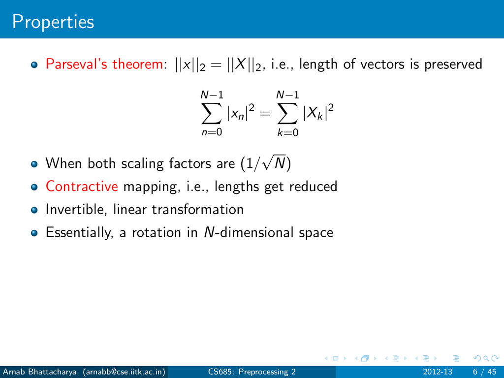
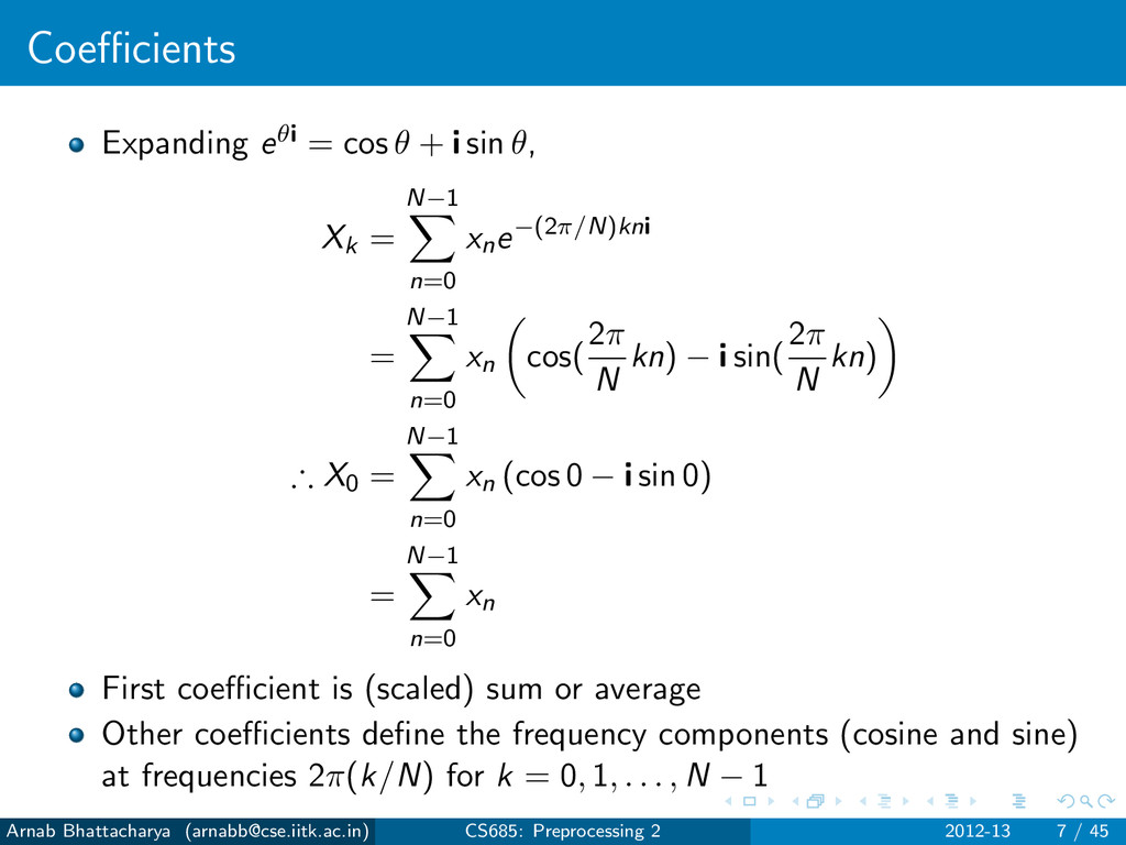
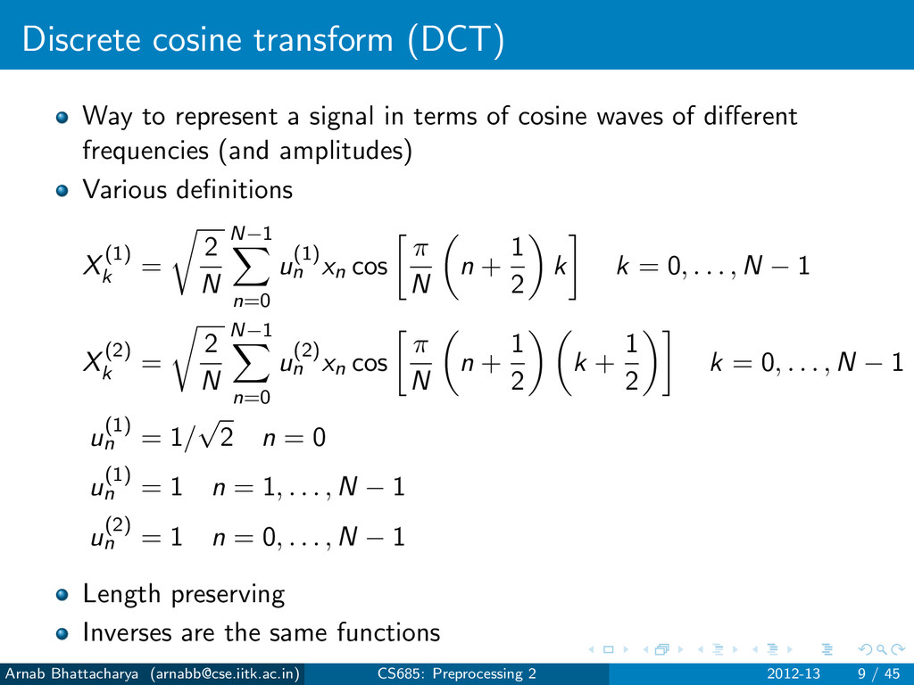
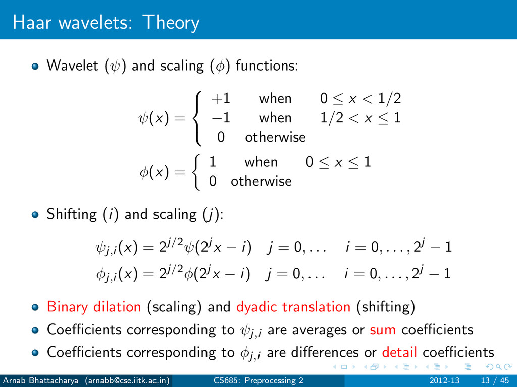
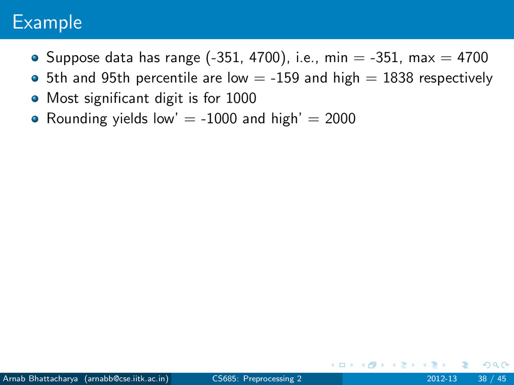
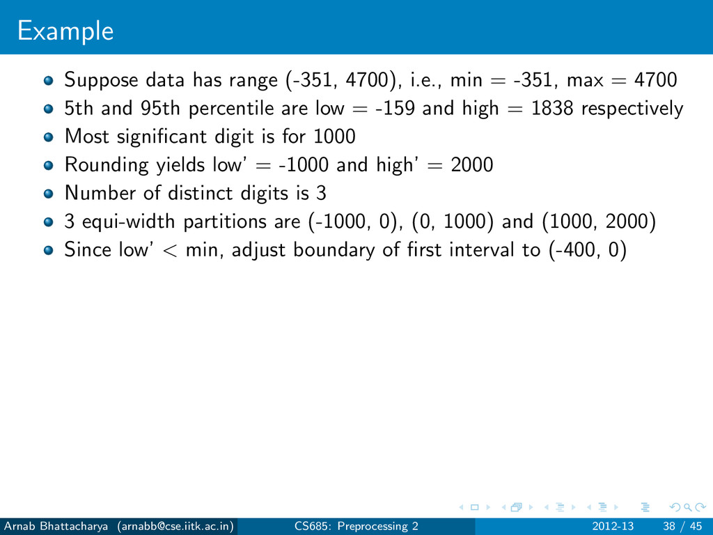
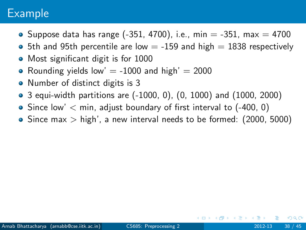
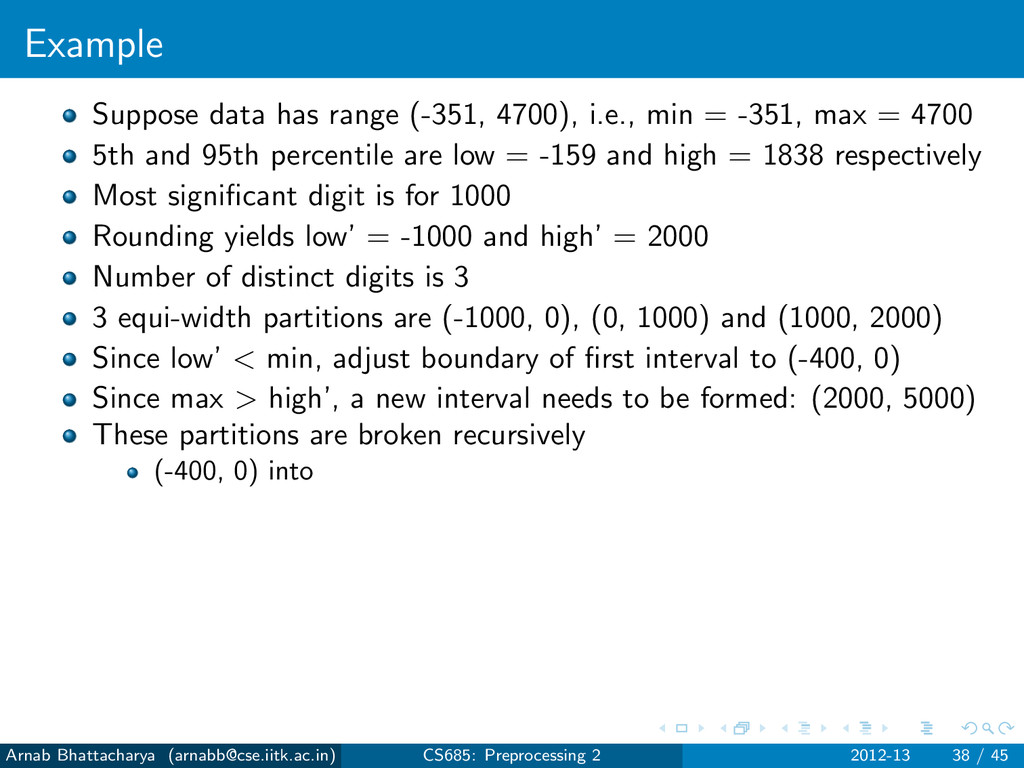
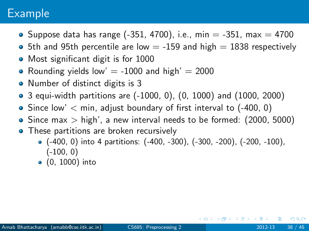
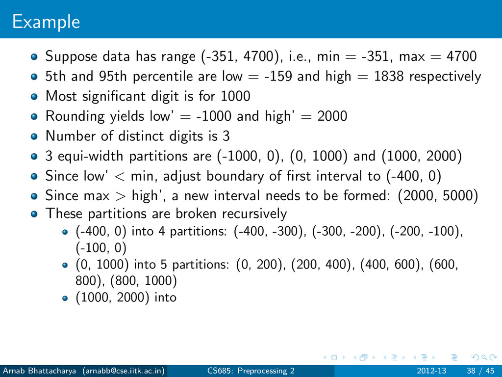
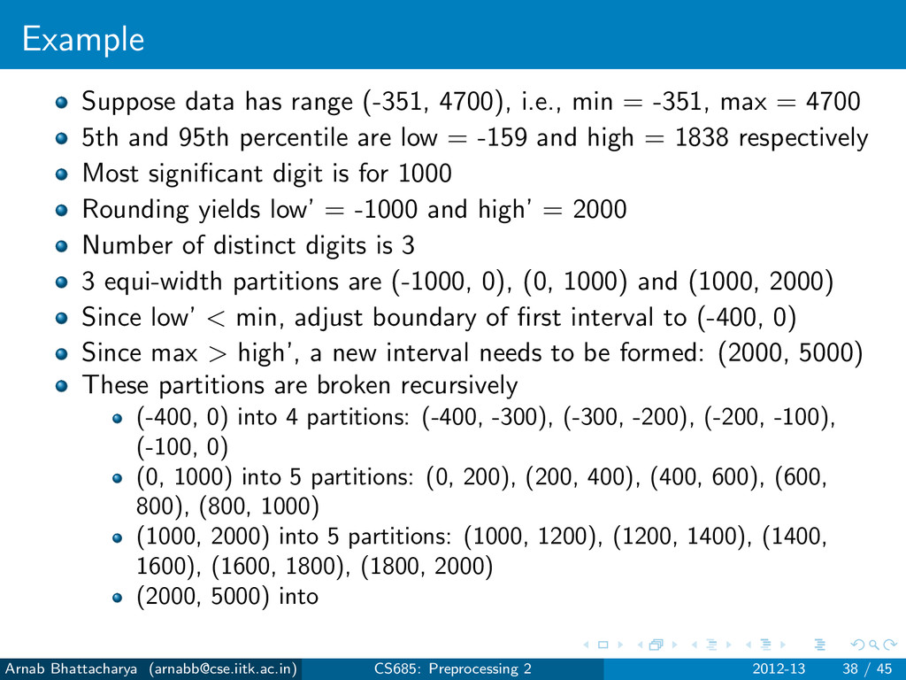
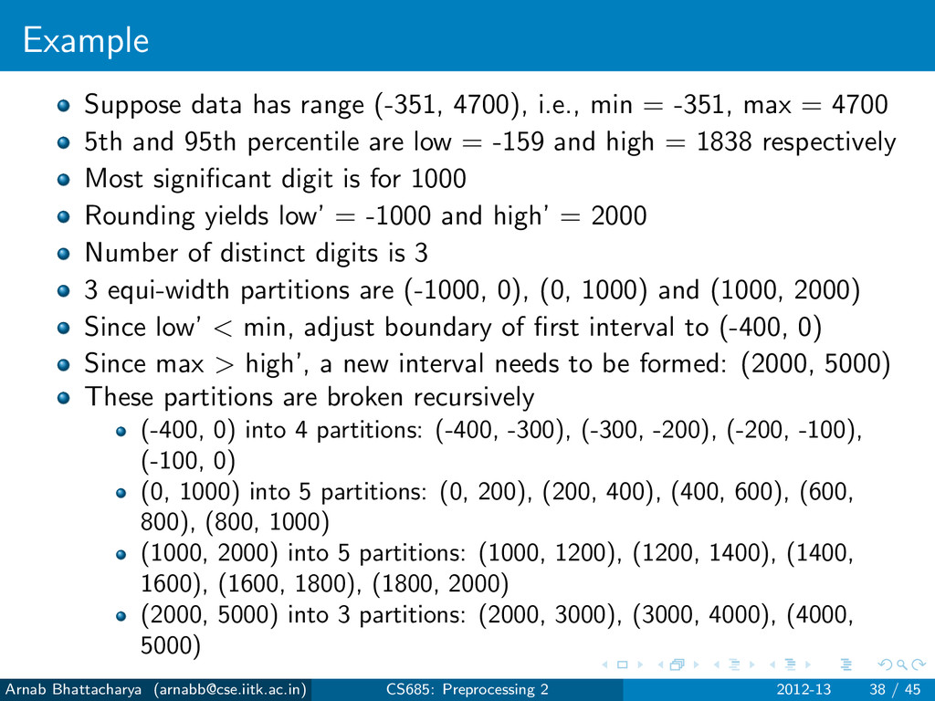
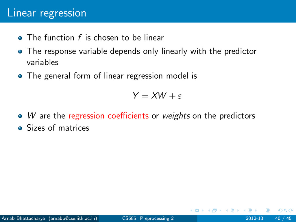
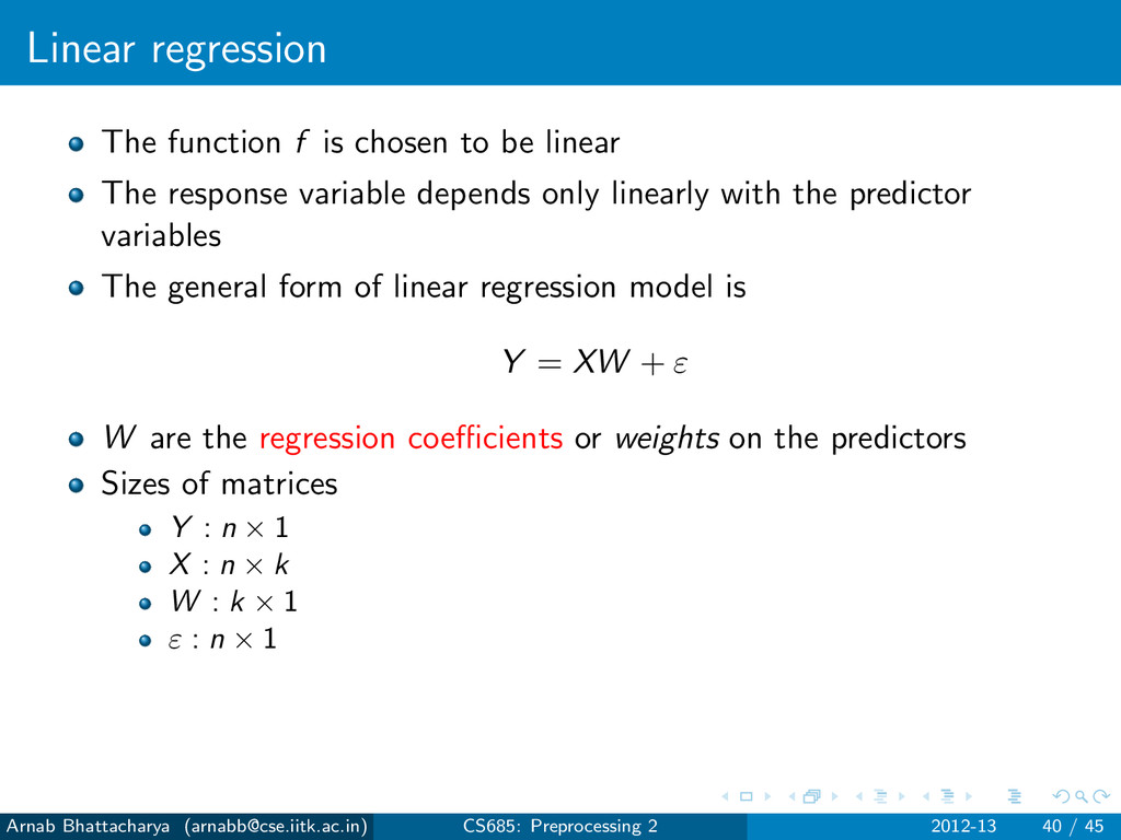
-351, max = 4700 5th and 95th percentile are low = -159 and high = 1838 respectively Most significant digit is for 1000 Rounding yields low’ = -1000 and high’ = 2000 Number of distinct digits is 3 3 equi-width partitions are (-1000, 0), (0, 1000) and (1000, 2000) Since low’ < min, adjust boundary of first interval to (-400, 0) Since max > high’, a new interval needs to be formed: (2000, 5000) These partitions are broken recursively (-400, 0) into 4 partitions: (-400, -300), (-300, -200), (-200, -100), (-100, 0) (0, 1000) into 5 partitions: (0, 200), (200, 400), (400, 600), (600, 800), (800, 1000) (1000, 2000) into 5 partitions: (1000, 1200), (1200, 1400), (1400, 1600), (1600, 1800), (1800, 2000) (2000, 5000) into 3 partitions: (2000, 3000), (3000, 4000), (4000, 5000) Arnab Bhattacharya (
[email protected]) CS685: Preprocessing 2 2012-13 38 / 45
![CS685: Data Mining Data Preprocessing Arnab Bhattacharya [email protected] Computer Science](https://files.speakerdeck.com/presentations/504ea2a2f2f61b0002032ebc/slide_0.jpg)
![Entropy Arnab Bhattacharya ([email protected]) CS685: Preprocessing 2 2012-13 23 /](https://files.speakerdeck.com/presentations/504ea2a2f2f61b0002032ebc/slide_30.jpg)
![Entropy-based discretization Supervised Top-down Arnab Bhattacharya ([email protected]) CS685: Preprocessing 2](https://files.speakerdeck.com/presentations/504ea2a2f2f61b0002032ebc/slide_39.jpg)
![Chi-merge discretization Supervised Bottom-up Arnab Bhattacharya ([email protected]) CS685: Preprocessing 2](https://files.speakerdeck.com/presentations/504ea2a2f2f61b0002032ebc/slide_56.jpg)
![Data transformation Data transformation is useful when Arnab Bhattacharya ([email protected])](https://files.speakerdeck.com/presentations/504ea2a2f2f61b0002032ebc/slide_86.jpg)
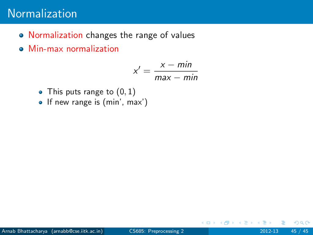
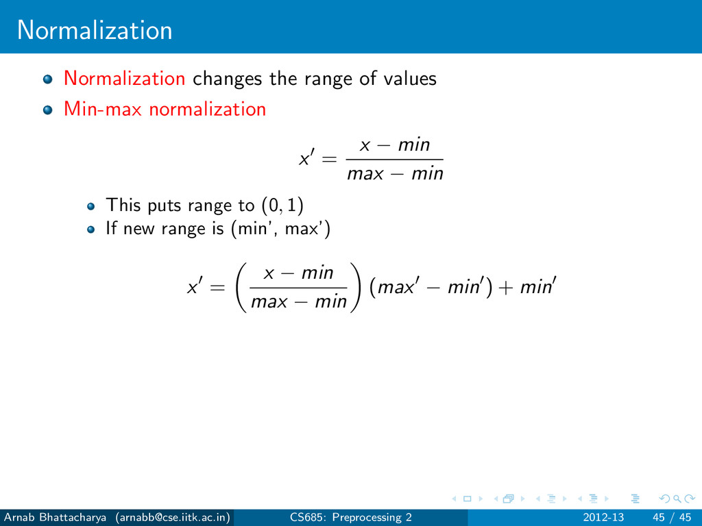
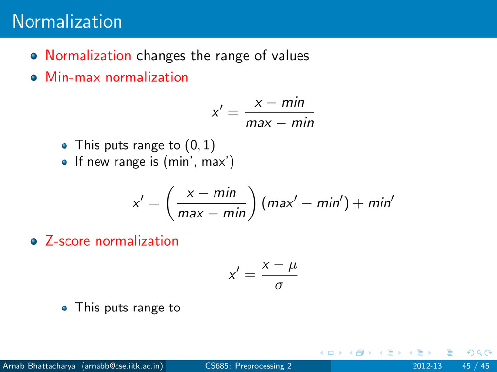
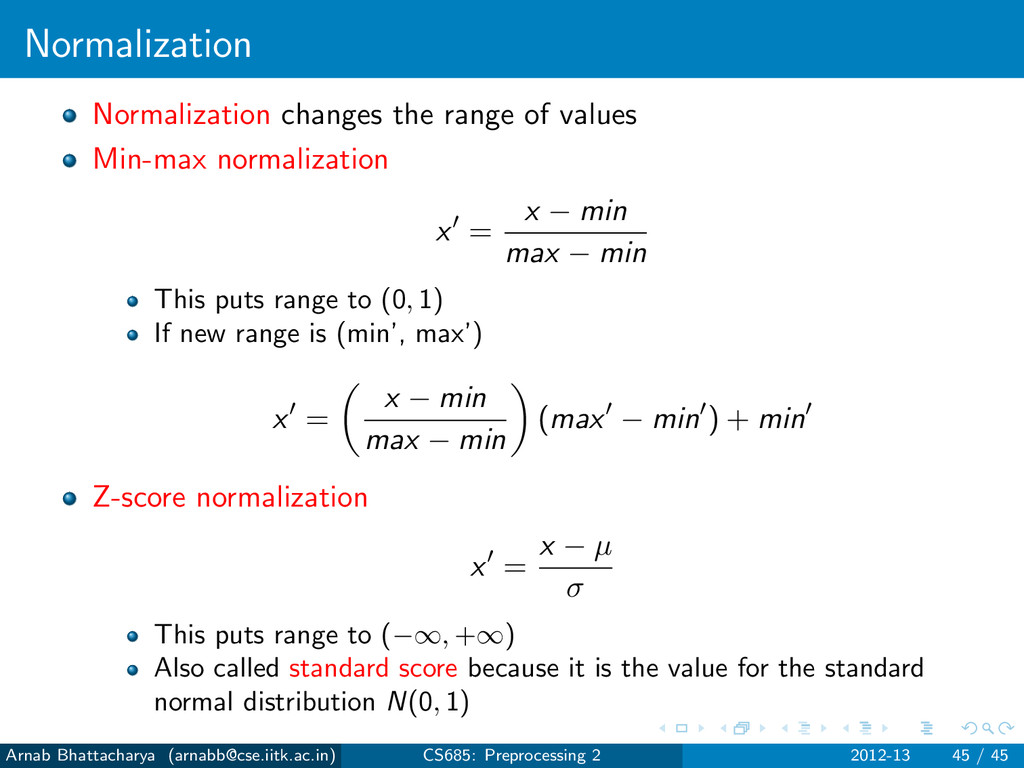
![Normalization Normalization changes the range of values Arnab Bhattacharya ([email protected])](https://files.speakerdeck.com/presentations/504ea2a2f2f61b0002032ebc/slide_89.jpg)