Testing galaxy formation models through the most massive objects in the universe

ASA meeting-Monash University, Melbourne 07/2013
Includes: comparison of BCGs growth observations with SAMs and halo occupation models. Cluster merger probes through non-central BCGs

Transcript

1.     Paola  Oliva-­‐Altamirano   Warrick  Couch,  Sarah  Brough,  Chris  Lidman   Testing galaxy formation models through the most massive objects in the universe  
3. OUTLINE   1.  BCG  M*  -­‐  Mhalo  relaHonship   3  
4. OUTLINE   1.  BCG  M*  -­‐  Mhalo  relaHonship   2.  BCG  Growth  over  cosmic  Hme   4  
5. OUTLINE   1.  BCG  M*  -­‐  Mhalo  relaHonship   2.  BCG  Growth  over  cosmic  Hme   4.  BCG  posiHon  in  the  cluster  
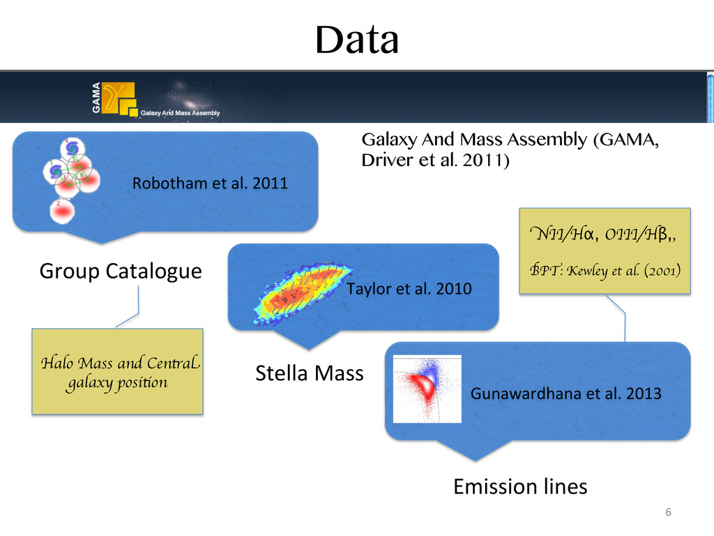
6. Data      Robotham  et  al.  2011   Group  Catalogue        Taylor  et  al.  2010   Stella  Mass            Gunawardhana  et  al.  2013   Emission  lines     Galaxy And Mass Assembly (GAMA, Driver et al. 2011) Halo Mass and Central galaxy position NII/Hα, OIII/Hβ,, BPT: Kewley et al. (2001) 6  
7. 7   BCG  M*   RaHo   RedshiS     1   1   Theory  
8. 8   BCG  M*   RaHo   RedshiS     1   1   ObservaHons   Theory  
9. 9   BCG  M*   RaHo   RedshiS     1   1   ObservaHons   Theory   Thanks  to  Lidman  et  al.  2012!  
11. Slope: 0.32 +/- 0.09 883 BCGs, group multiplicity >5, 0.09 < z < 0.27   Previous work: Lin & Mohr (2004): z < 0.09, ~0.26 Brough et al. (2008): z < 0.1, ~0.24 Hansen et al. (2009): 0.1 < z < 0.3, ~0.3 11   BCG  M*  -­‐  Mhalo  relaHonship  
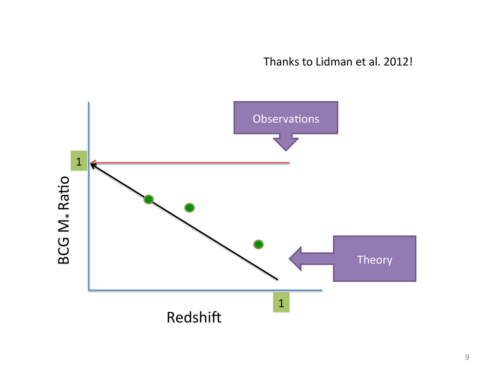
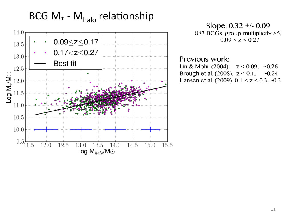
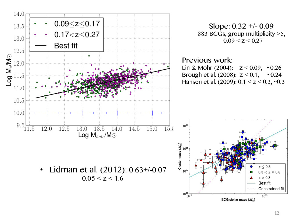
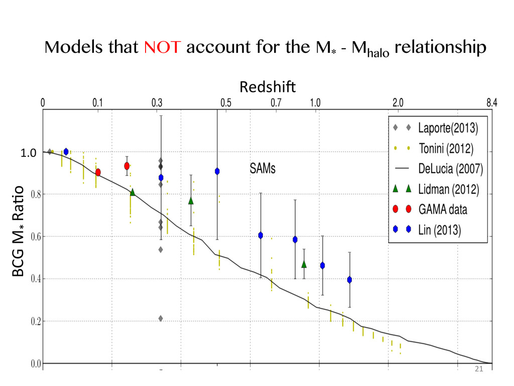
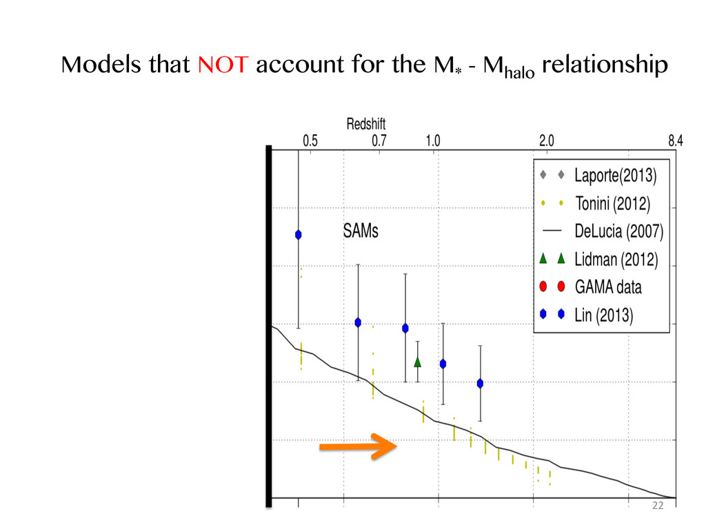
12. Slope: 0.32 +/- 0.09 883 BCGs, group multiplicity >5, 0.09 < z < 0.27   Previous work: Lin & Mohr (2004): z < 0.09, ~0.26 Brough et al. (2008): z < 0.1, ~0.24 Hansen et al. (2009): 0.1 < z < 0.3, ~0.3 •  Lidman et al. (2012): 0.63+/-0.07 0.05 < z < 1.6 12  
14. Does this relationship evolves With redshift? 14  
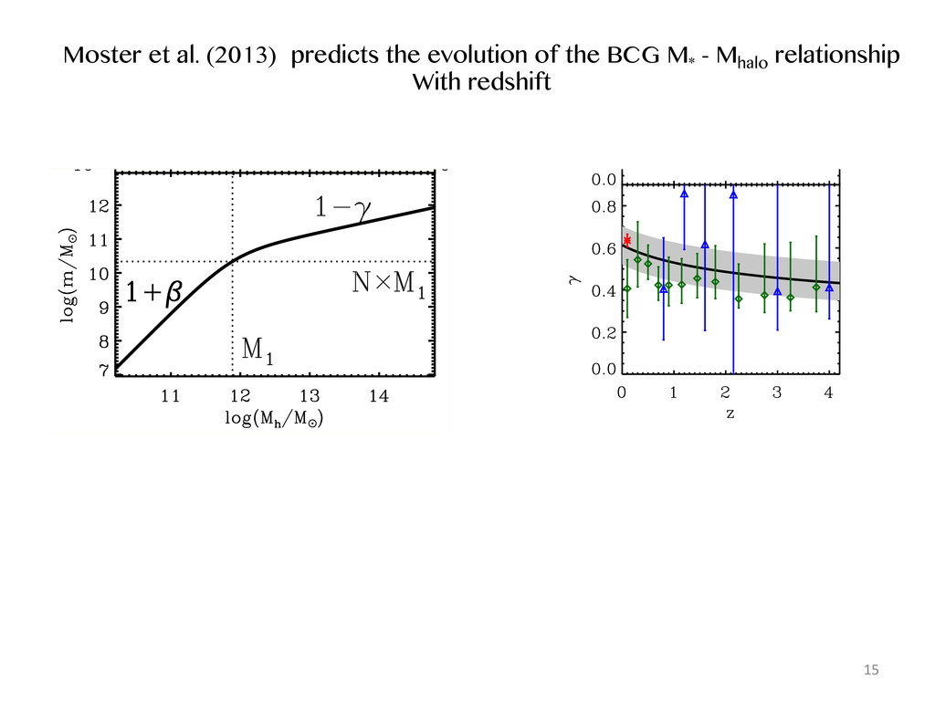
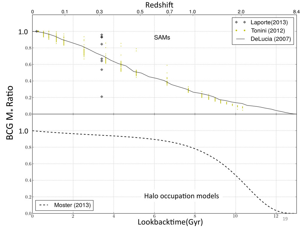
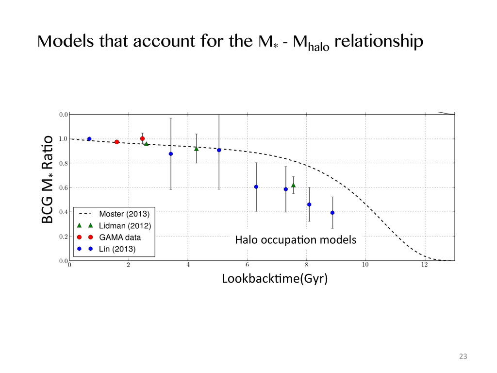
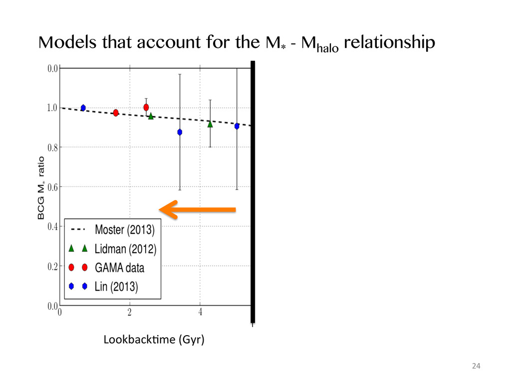
15. - s - e d f s - - - . d d - w f . a - - - a r t t p f s m , n - I Figure 1. Upper panel: Sketch of the stellar-to-halo mass ratio as a function of halo mass peaking around the characteristic mass M1 where it has the normalization N. It has a low-mass slope β and a high mass slope −γ. Lower panel: Sketch of the stellar-to- halo mass relation as a function of halo mass. The low-mass slope is 1 + β and the high mass slope is 1 − γ. Moster et al. (2010): m = 2 N M −β + M γ −1 . (2) Figure 2. Evolution of the SHM relation parameters with redshift in a model without observational mass errors. The symbols correspond to the values that have been derived with the classical abundance matching approach at individual redshifts. Different colors represent the different SMFs that have been used to derive the SHM relation: red crosses for the SDSS SMF, green diamonds for the PG08 SMFs and blue triangles for the S12 SMFs. The solid line corresponds to a multi-epoch abundance matching model that takes into account that satellites are accreted at different epochs. The shaded area indicates the 1σ confidence levels. For M1 and N we assume a second order polynomial in z and for β and γ a power law in z. 3.1 The evolution of the stellar-to-halo mass relation As a first step, we investigate how the parameters of the SHM relation evolve with redshift. For this we assume that at a given redshift the relation between the stellar mass of a satellite galaxy and the maximum mass of its dark mat- ter halo over its history is the same as the SHM relation of central galaxies. This assumption is only an approximation as the stellar mass of satellites is related to the halo mass at infall and the SHM relation is expected to have changed by relating it to the observed SMF at this redshift: L = exp −χ2 r χ2 r = 1 NΦ NΦ i=1 log Φmod (mi) − log Φobs (mi) σobs (mi) 2 . (4) Employing a Markov chain Monte Carlo (MCMC) method, we sample the probability distribution for the parameters and extract the best-fit values and their 1σ errors. We repeat this procedure for every observed SMF available and plot the Moster et al. (2013) predicts the evolution of the BCG M* - Mhalo relationship With redshift 15  
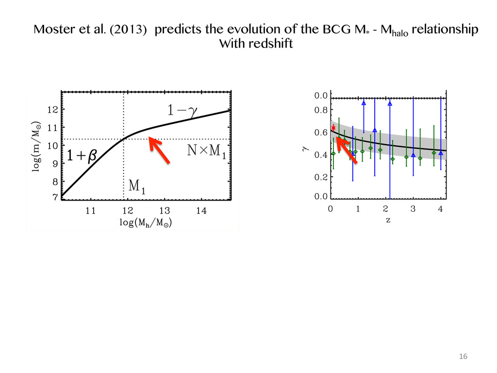
16. - s - e d f s - - - . d d - w f . a - - - a r t t p f s m , n - I Figure 1. Upper panel: Sketch of the stellar-to-halo mass ratio as a function of halo mass peaking around the characteristic mass M1 where it has the normalization N. It has a low-mass slope β and a high mass slope −γ. Lower panel: Sketch of the stellar-to- halo mass relation as a function of halo mass. The low-mass slope is 1 + β and the high mass slope is 1 − γ. Moster et al. (2010): m = 2 N M −β + M γ −1 . (2) Figure 2. Evolution of the SHM relation parameters with redshift in a model without observational mass errors. The symbols correspond to the values that have been derived with the classical abundance matching approach at individual redshifts. Different colors represent the different SMFs that have been used to derive the SHM relation: red crosses for the SDSS SMF, green diamonds for the PG08 SMFs and blue triangles for the S12 SMFs. The solid line corresponds to a multi-epoch abundance matching model that takes into account that satellites are accreted at different epochs. The shaded area indicates the 1σ confidence levels. For M1 and N we assume a second order polynomial in z and for β and γ a power law in z. 3.1 The evolution of the stellar-to-halo mass relation As a first step, we investigate how the parameters of the SHM relation evolve with redshift. For this we assume that at a given redshift the relation between the stellar mass of a satellite galaxy and the maximum mass of its dark mat- ter halo over its history is the same as the SHM relation of central galaxies. This assumption is only an approximation as the stellar mass of satellites is related to the halo mass at infall and the SHM relation is expected to have changed by relating it to the observed SMF at this redshift: L = exp −χ2 r χ2 r = 1 NΦ NΦ i=1 log Φmod (mi) − log Φobs (mi) σobs (mi) 2 . (4) Employing a Markov chain Monte Carlo (MCMC) method, we sample the probability distribution for the parameters and extract the best-fit values and their 1σ errors. We repeat this procedure for every observed SMF available and plot the Moster et al. (2013) predicts the evolution of the BCG M* - Mhalo relationship With redshift 16  
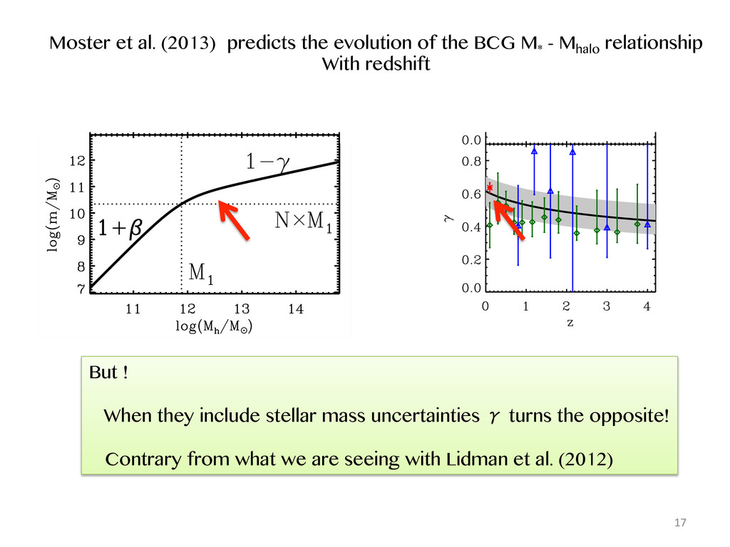
17. - s - e d f s - - - . d d - w f . a - - - a r t t p f s m , n - I Figure 1. Upper panel: Sketch of the stellar-to-halo mass ratio as a function of halo mass peaking around the characteristic mass M1 where it has the normalization N. It has a low-mass slope β and a high mass slope −γ. Lower panel: Sketch of the stellar-to- halo mass relation as a function of halo mass. The low-mass slope is 1 + β and the high mass slope is 1 − γ. Moster et al. (2010): m = 2 N M −β + M γ −1 . (2) Figure 2. Evolution of the SHM relation parameters with redshift in a model without observational mass errors. The symbols correspond to the values that have been derived with the classical abundance matching approach at individual redshifts. Different colors represent the different SMFs that have been used to derive the SHM relation: red crosses for the SDSS SMF, green diamonds for the PG08 SMFs and blue triangles for the S12 SMFs. The solid line corresponds to a multi-epoch abundance matching model that takes into account that satellites are accreted at different epochs. The shaded area indicates the 1σ confidence levels. For M1 and N we assume a second order polynomial in z and for β and γ a power law in z. 3.1 The evolution of the stellar-to-halo mass relation As a first step, we investigate how the parameters of the SHM relation evolve with redshift. For this we assume that at a given redshift the relation between the stellar mass of a satellite galaxy and the maximum mass of its dark mat- ter halo over its history is the same as the SHM relation of central galaxies. This assumption is only an approximation as the stellar mass of satellites is related to the halo mass at infall and the SHM relation is expected to have changed by relating it to the observed SMF at this redshift: L = exp −χ2 r χ2 r = 1 NΦ NΦ i=1 log Φmod (mi) − log Φobs (mi) σobs (mi) 2 . (4) Employing a Markov chain Monte Carlo (MCMC) method, we sample the probability distribution for the parameters and extract the best-fit values and their 1σ errors. We repeat this procedure for every observed SMF available and plot the Moster et al. (2013) predicts the evolution of the BCG M* - Mhalo relationship With redshift But ! When they include stellar mass uncertainties γ turns the opposite! Contrary from what we are seeing with Lidman et al. (2012) 17  
18. After matching cluster according to Mass... We find : BCGs have not grown in M* in the last 3 billion years!! M* low-z/M* low-z ~1 18  
19. RedshiS   LookbackHme(Gyr)   BCG  M*   RaHo   1.0   1.0   19   Halo  occupaHon  models  
20. RedshiS   LookbackHme(Gyr)   BCG  M*   RaHo   1.0   1.0   20   Halo  occupaHon  models   Galactic star formation and accretion histor Figure 7. Left panels: Average fraction of z = 0 mass assembled as a function of redshift for dark matter haloes (blue d and central galaxies (red solid lines). Each panel compares the mass assembly history of a central galaxy to that of its pare z = 0 halo and stellar masses are indicated in each panel. While for low-mass dark matter haloes most of the mass assem times, massive haloes only assemble late. For galaxies these trends are opposite. Right panel: Average formation redshift of haloes (blue dashed lines) and central galaxies (red solid lines) as a function of z = 0 mass. The three different lines indicate at which 25, 50, and 75 per cent of the mass was in place. of the central galaxy forms after redshift z = 0.7 while half of the virial mass was already assembled by redshift z = 1.3. that formed outside the galaxy and have been ac (ex-situ). In principle, both processes can contri
21. Models that NOT account for the M* - Mhalo relationship 1.0   RedshiS   BCG  M*   RaHo   21  
22. Models that NOT account for the M* - Mhalo relationship 22  
23. Models that account for the M* - Mhalo relationship BCG  M*   RaHo   LookbackHme(Gyr)   23   Halo  occupaHon  models  
24. Models that account for the M* - Mhalo relationship LookbackHme  (Gyr)   24  
25. BCGs acquire their mass rapidly at early epochs But slow down in the last 5 billion years 25  
26. BCG Position in the Cluster… 14% of the BCGs are NOT At the centre of the cluster 26  
27. The fraction of central BCGs decreases with MHalo In  agreement  with   Skibba  et  al.  2011     Results.    
28. How different are cenBCGs from non-cenBCGs? Dominance:  difference     In  magnitude  between   The  BCG  and  the  2nd     Brightest  galaxy  of  the   Cluster.   RelaHve  Overdensity:   Density  of  the  cluster    environment.        
29. How different are cenBCGs from non-cenBCGs? Dominance:  difference     In  magnitude  between   The  BCG  and  the  2nd     Brightest  galaxy  of  the   Cluster.   RelaHve  Overdensity:   Density  of  the  cluster    environment.        
30. cenBCGs are more massive than non-cenBCGs ~0.3  dex  
31. The fact that some BCGs are not at the centre of the Halo is a probe of mergers between clusters 31  
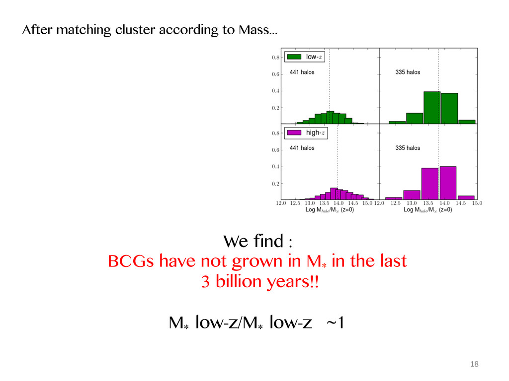
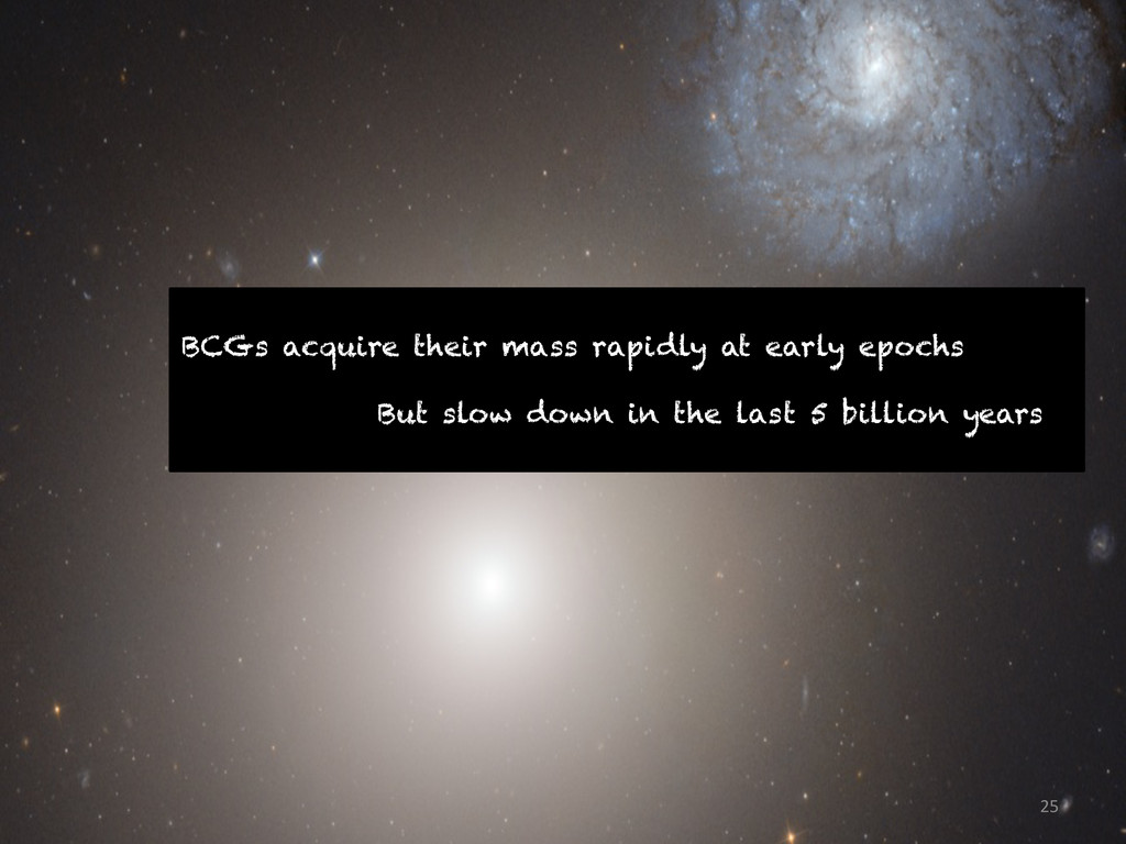
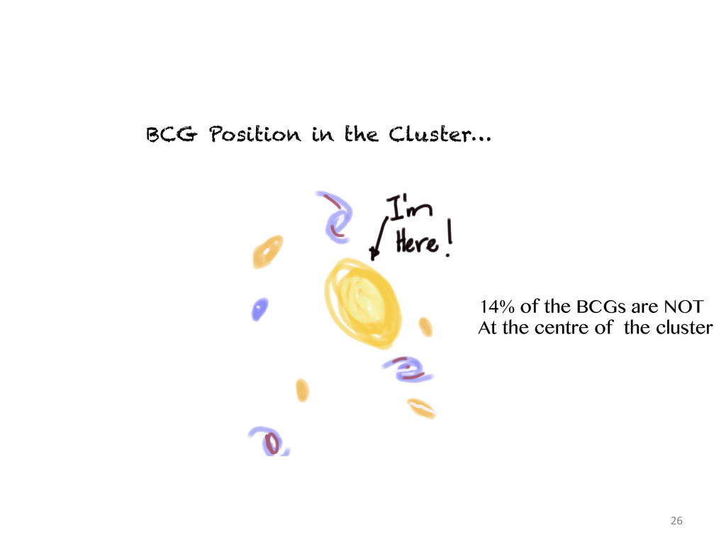
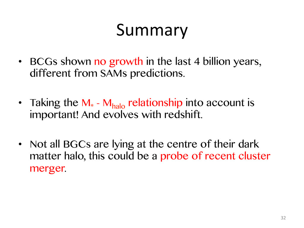
32. Summary   •  BCGs shown no growth in the last 4 billion years, different from SAMs predictions. •  Taking the M* - Mhalo relationship into account is important! And evolves with redshift. •  Not all BGCs are lying at the centre of their dark matter halo, this could be a probe of recent cluster merger. 32  
33. QuesHons,      SuggesHons…