BCGs as Probes of Galaxy Formation

On the growth of BCGs through cosmic time. A comparison between models and observations. We also covered BCG star formation and AGN activity in the last 3 billion years.

Transcript

1.     Paola  Oliva-­‐Altamirano   Warrick  Couch,  Sarah  Brough,  Chris  Lidman   Growing the most massive objects in the universe:   How well do galaxy formation models match observations?  
3. OUTLINE   1.  BCG  M*  -­‐  Mhalo  relaHonship   3  
4. OUTLINE   1.  BCG  M*  -­‐  Mhalo  relaHonship   2.  BCG  Growth  over  cosmic  Hme   4  
5. OUTLINE   1.  BCG  M*  -­‐  Mhalo  relaHonship   2.  BCG  Growth  over  cosmic  Hme   3.  BCG  AGN  and  star  formaHon  acHvity   5  
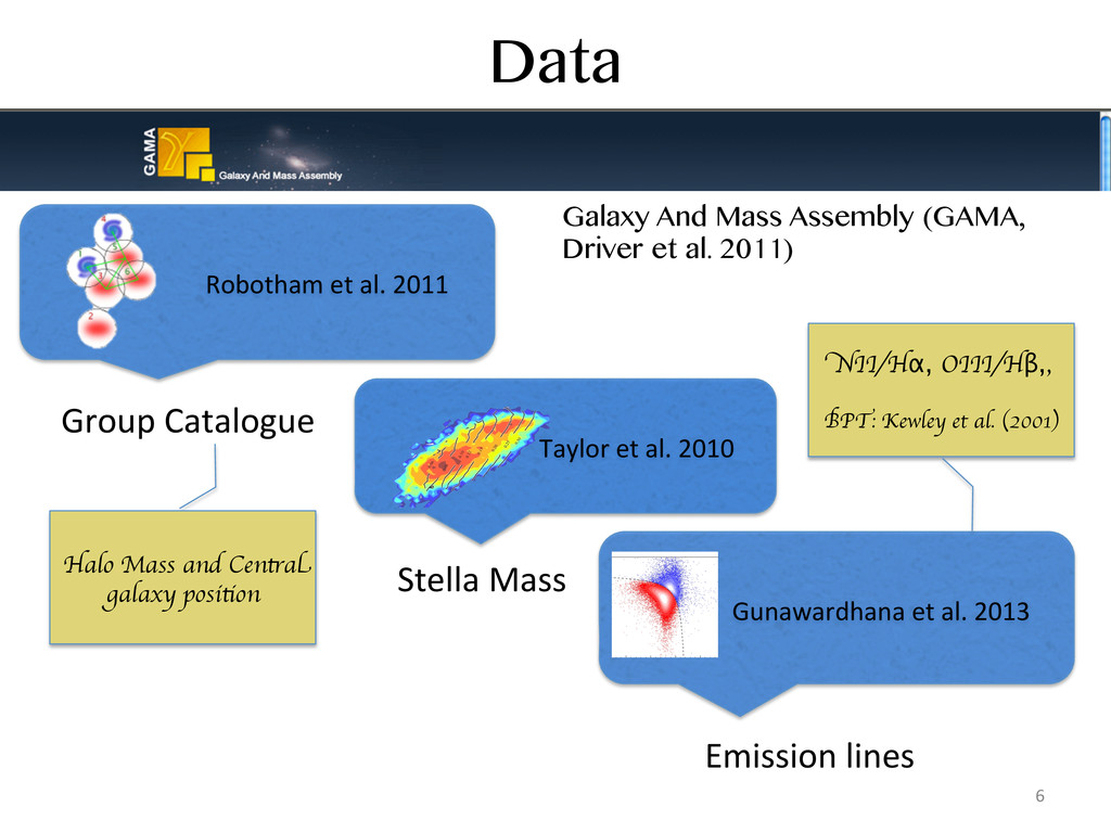
6. Data      Robotham  et  al.  2011   Group  Catalogue        Taylor  et  al.  2010   Stella  Mass            Gunawardhana  et  al.  2013   Emission  lines     Galaxy And Mass Assembly (GAMA, Driver et al. 2011) Halo Mass and Central galaxy position NII/Hα, OIII/Hβ,, BPT: Kewley et al. (2001) 6  
7. Slope: 0.32 +/- 0.09 883 BCGs, group multiplicity >5, 0.09 < z < 0.27   Previous work: Lin & Mohr (2004): z < 0.09, ~0.26 Brough et al. (2008): z < 0.1, ~0.24 Hansen et al. (2009): 0.1 < z < 0.3, ~0.3 7  
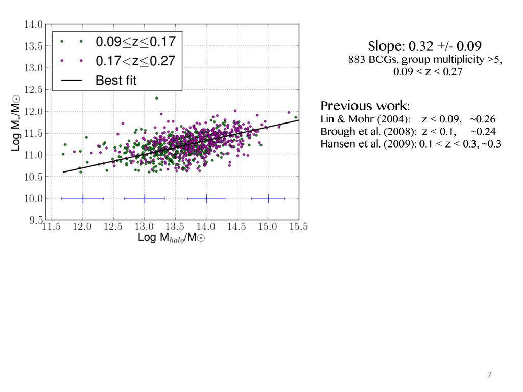
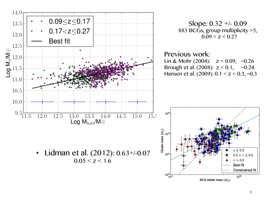
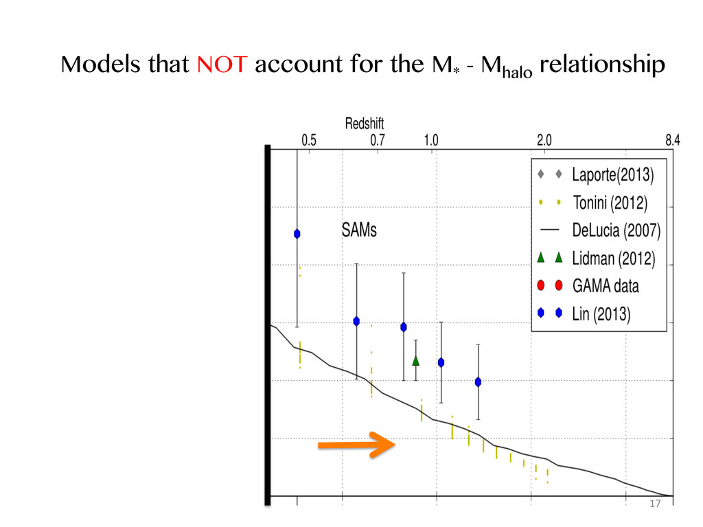
8. Slope: 0.32 +/- 0.09 883 BCGs, group multiplicity >5, 0.09 < z < 0.27   Previous work: Lin & Mohr (2004): z < 0.09, ~0.26 Brough et al. (2008): z < 0.1, ~0.24 Hansen et al. (2009): 0.1 < z < 0.3, ~0.3 •  Lidman et al. (2012): 0.63+/-0.07 0.05 < z < 1.6 8  
10. Does this relationship evolves With redshift? 10  
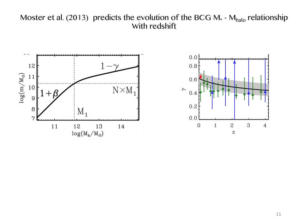
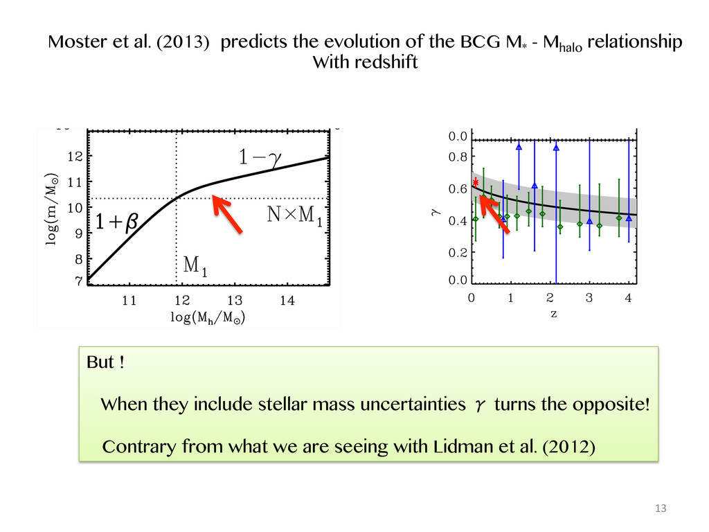
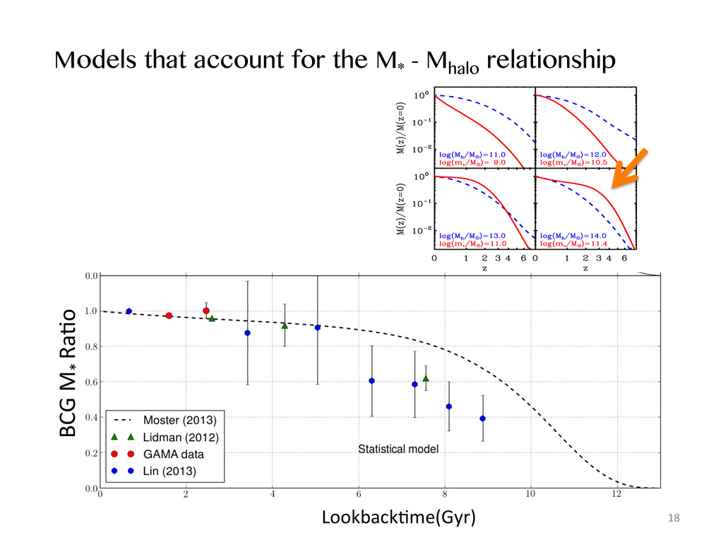
11. - s - e d f s - - - . d d - w f . a - - - a r t t p f s m , n - I Figure 1. Upper panel: Sketch of the stellar-to-halo mass ratio as a function of halo mass peaking around the characteristic mass M1 where it has the normalization N. It has a low-mass slope β and a high mass slope −γ. Lower panel: Sketch of the stellar-to- halo mass relation as a function of halo mass. The low-mass slope is 1 + β and the high mass slope is 1 − γ. Moster et al. (2010): m = 2 N M −β + M γ −1 . (2) Figure 2. Evolution of the SHM relation parameters with redshift in a model without observational mass errors. The symbols correspond to the values that have been derived with the classical abundance matching approach at individual redshifts. Different colors represent the different SMFs that have been used to derive the SHM relation: red crosses for the SDSS SMF, green diamonds for the PG08 SMFs and blue triangles for the S12 SMFs. The solid line corresponds to a multi-epoch abundance matching model that takes into account that satellites are accreted at different epochs. The shaded area indicates the 1σ confidence levels. For M1 and N we assume a second order polynomial in z and for β and γ a power law in z. 3.1 The evolution of the stellar-to-halo mass relation As a first step, we investigate how the parameters of the SHM relation evolve with redshift. For this we assume that at a given redshift the relation between the stellar mass of a satellite galaxy and the maximum mass of its dark mat- ter halo over its history is the same as the SHM relation of central galaxies. This assumption is only an approximation as the stellar mass of satellites is related to the halo mass at infall and the SHM relation is expected to have changed by relating it to the observed SMF at this redshift: L = exp −χ2 r χ2 r = 1 NΦ NΦ i=1 log Φmod (mi) − log Φobs (mi) σobs (mi) 2 . (4) Employing a Markov chain Monte Carlo (MCMC) method, we sample the probability distribution for the parameters and extract the best-fit values and their 1σ errors. We repeat this procedure for every observed SMF available and plot the Moster et al. (2013) predicts the evolution of the BCG M* - Mhalo relationship With redshift 11  
12. - s - e d f s - - - . d d - w f . a - - - a r t t p f s m , n - I Figure 1. Upper panel: Sketch of the stellar-to-halo mass ratio as a function of halo mass peaking around the characteristic mass M1 where it has the normalization N. It has a low-mass slope β and a high mass slope −γ. Lower panel: Sketch of the stellar-to- halo mass relation as a function of halo mass. The low-mass slope is 1 + β and the high mass slope is 1 − γ. Moster et al. (2010): m = 2 N M −β + M γ −1 . (2) Figure 2. Evolution of the SHM relation parameters with redshift in a model without observational mass errors. The symbols correspond to the values that have been derived with the classical abundance matching approach at individual redshifts. Different colors represent the different SMFs that have been used to derive the SHM relation: red crosses for the SDSS SMF, green diamonds for the PG08 SMFs and blue triangles for the S12 SMFs. The solid line corresponds to a multi-epoch abundance matching model that takes into account that satellites are accreted at different epochs. The shaded area indicates the 1σ confidence levels. For M1 and N we assume a second order polynomial in z and for β and γ a power law in z. 3.1 The evolution of the stellar-to-halo mass relation As a first step, we investigate how the parameters of the SHM relation evolve with redshift. For this we assume that at a given redshift the relation between the stellar mass of a satellite galaxy and the maximum mass of its dark mat- ter halo over its history is the same as the SHM relation of central galaxies. This assumption is only an approximation as the stellar mass of satellites is related to the halo mass at infall and the SHM relation is expected to have changed by relating it to the observed SMF at this redshift: L = exp −χ2 r χ2 r = 1 NΦ NΦ i=1 log Φmod (mi) − log Φobs (mi) σobs (mi) 2 . (4) Employing a Markov chain Monte Carlo (MCMC) method, we sample the probability distribution for the parameters and extract the best-fit values and their 1σ errors. We repeat this procedure for every observed SMF available and plot the Moster et al. (2013) predicts the evolution of the BCG M* - Mhalo relationship With redshift 12  
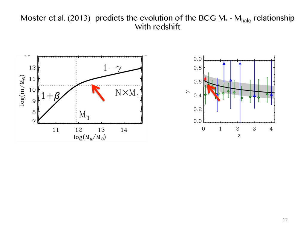
13. - s - e d f s - - - . d d - w f . a - - - a r t t p f s m , n - I Figure 1. Upper panel: Sketch of the stellar-to-halo mass ratio as a function of halo mass peaking around the characteristic mass M1 where it has the normalization N. It has a low-mass slope β and a high mass slope −γ. Lower panel: Sketch of the stellar-to- halo mass relation as a function of halo mass. The low-mass slope is 1 + β and the high mass slope is 1 − γ. Moster et al. (2010): m = 2 N M −β + M γ −1 . (2) Figure 2. Evolution of the SHM relation parameters with redshift in a model without observational mass errors. The symbols correspond to the values that have been derived with the classical abundance matching approach at individual redshifts. Different colors represent the different SMFs that have been used to derive the SHM relation: red crosses for the SDSS SMF, green diamonds for the PG08 SMFs and blue triangles for the S12 SMFs. The solid line corresponds to a multi-epoch abundance matching model that takes into account that satellites are accreted at different epochs. The shaded area indicates the 1σ confidence levels. For M1 and N we assume a second order polynomial in z and for β and γ a power law in z. 3.1 The evolution of the stellar-to-halo mass relation As a first step, we investigate how the parameters of the SHM relation evolve with redshift. For this we assume that at a given redshift the relation between the stellar mass of a satellite galaxy and the maximum mass of its dark mat- ter halo over its history is the same as the SHM relation of central galaxies. This assumption is only an approximation as the stellar mass of satellites is related to the halo mass at infall and the SHM relation is expected to have changed by relating it to the observed SMF at this redshift: L = exp −χ2 r χ2 r = 1 NΦ NΦ i=1 log Φmod (mi) − log Φobs (mi) σobs (mi) 2 . (4) Employing a Markov chain Monte Carlo (MCMC) method, we sample the probability distribution for the parameters and extract the best-fit values and their 1σ errors. We repeat this procedure for every observed SMF available and plot the Moster et al. (2013) predicts the evolution of the BCG M* - Mhalo relationship With redshift But ! When they include stellar mass uncertainties γ turns the opposite! Contrary from what we are seeing with Lidman et al. (2012) 13  
14. After matching cluster according to Mass... We find : BCGs have not grown in M* in the last 3 billion years!! M* low-z/M* low-z ~1 14  
15. RedshiW   LookbackHme(Gyr)   BCG  M*   RaHo   1.0   1.0   15  
16. Models that NOT account for the M* - Mhalo relationship 1.0   RedshiW   BCG  M*   RaHo   16  
17. Models that NOT account for the M* - Mhalo relationship 17  
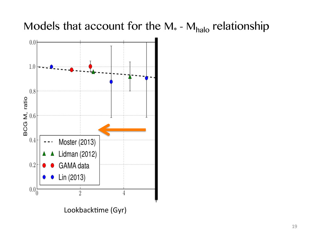
18. Models that account for the M* - Mhalo relationship Galactic star formati Figure 7. Left panels: Average fraction of z = 0 mass assembled as a function of redshift and central galaxies (red solid lines). Each panel compares the mass assembly history of a c z = 0 halo and stellar masses are indicated in each panel. While for low-mass dark matter times, massive haloes only assemble late. For galaxies these trends are opposite. Right pane haloes (blue dashed lines) and central galaxies (red solid lines) as a function of z = 0 mass. T at which 25, 50, and 75 per cent of the mass was in place. of the central galaxy forms after redshift z = 0.7 while half of the virial mass was already assembled by redshift z = 1.3. In more massive systems haloes assemble later while galax- ies assemble earlier: for a system with a z = 0 halo mass of Mvir = 1013M , half of the halo has assembled only by redshift z = 1.0, but half of the stellar mass was already in place by redshift z = 1.8. Very massive galaxies in haloes with Mvir = 1014M show a very interesting behavior: while they begin to form very early and have 25 per cent of their stellar mass in place already by redshift z = 3.0, it takes them a long time to fully assemble. Half of their stellar mass is in place only by red- shift z = 1.6, while 75 per cent is assembled by z = 0.3. The final z = 0 stellar mass is then assembled very quickly. The reason why these massive galaxies grow very fast at early times, only grow slowly at intermediate redshifts and grow fast again at late times can be found in the two processes that contribute to the growth of galaxies. At high redshift, a massive galaxy grows effectively by star formation, while at low redshift, stellar accretion leads to a fast growth. At that formed outsid (ex-situ). In princip taneously to the gr one process will dom mass and redshift. from star formatio mine the amount o object in the halo. these subhaloes wit lar accretion rate. F the difference betw tion rate. We use the sa as before, i.e. we u mass of the main h and subhaloes usin For every simulatio galaxies that are a time of the next sn BCG  M*   RaHo   LookbackHme(Gyr)   18  
19. Models that account for the M* - Mhalo relationship LookbackHme  (Gyr)   19  
20. BCGs acquire their mass rapidly at early epochs But slow down in the last 4 billion years 20  
21. BCGs Star formation and AGN activity in the last 3 billion years 21  
22. AGN fraction remains fairly constant SF Decreases with Stellar Mass 22  
23. From the BCGs that are star Forming (235 out 883) 23   Log  SFR  [Msun /yr]  
24. From the BCGs that are star Forming (235 out 883) Yang et al. SF   Bimodal   Quenched   Yang  et  al.  2013   24   Log  SFR  [Msun /yr]  
25. Star  FormaHon  inclusion  can  improve  photometric  colors!   See  Chiara  Tonini’s  Talk  later        or              Tonini  et  al.(2012)   25  
26. BCG Position in the Cluster… 14% of the BCGs are NOT At the centre of the cluster 26  
27. The fact that some BCGs are not at the centre of the Halo is a probe of mergers between clusters 27   See  talk  in  the  ASA  next  week     Stay  tuned  for  Oliva-­‐Altamirano  (in  prep.)   Talk  to  me  later!!!  
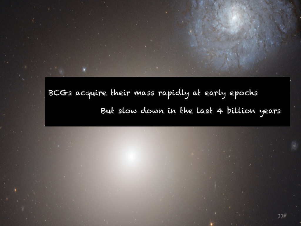
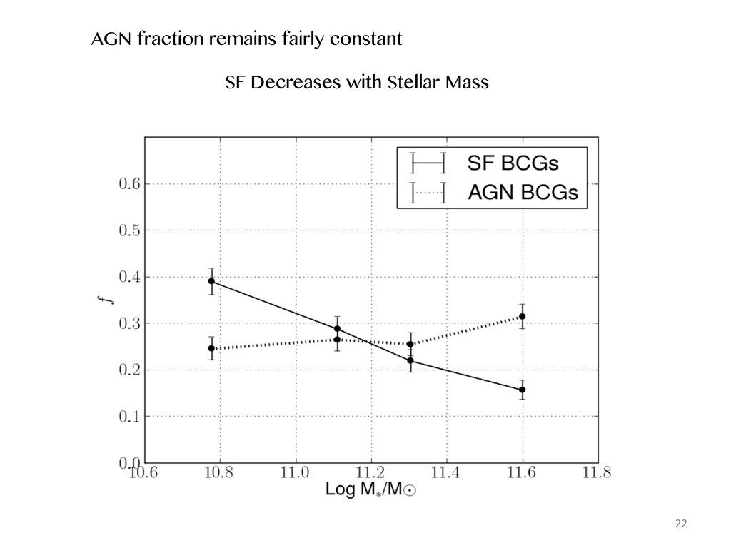
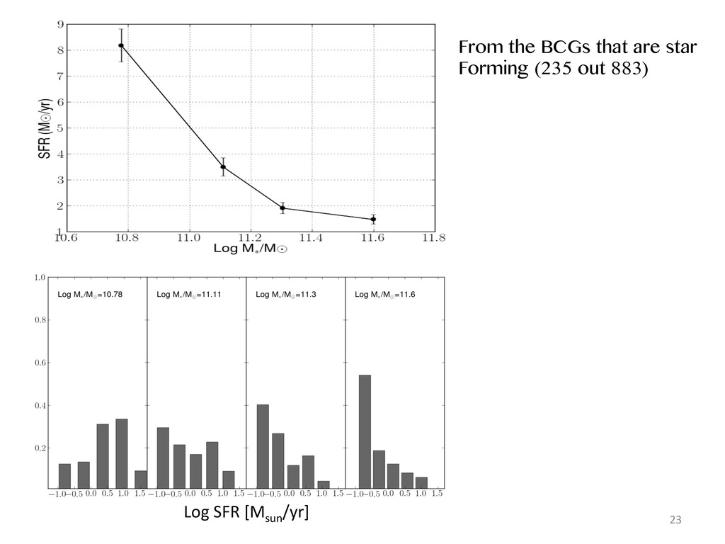
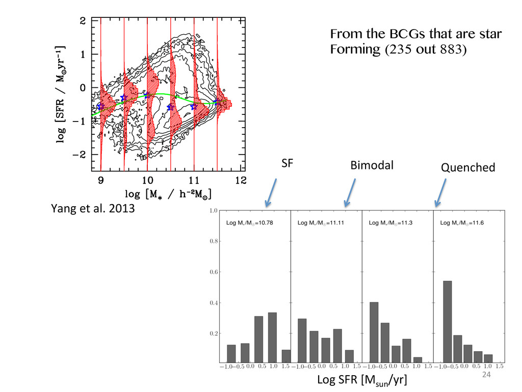
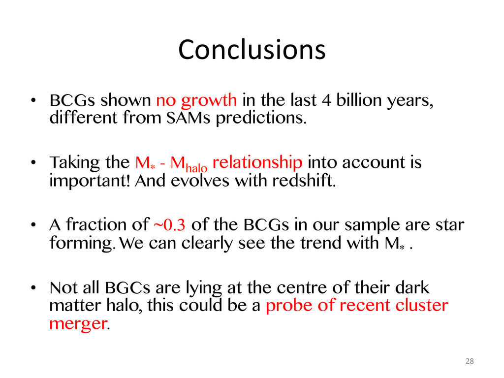
28. Conclusions   •  BCGs shown no growth in the last 4 billion years, different from SAMs predictions. •  Taking the M* - Mhalo relationship into account is important! And evolves with redshift. •  A fraction of ~0.3 of the BCGs in our sample are star forming. We can clearly see the trend with M* . •  Not all BGCs are lying at the centre of their dark matter halo, this could be a probe of recent cluster merger. 28