Upgrade to Pro — share decks privately, control downloads, hide ads and more …

Sea-level Variability and Predictability: USAPI

Sea-level Variability and Predictability: USAPI

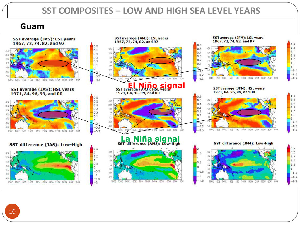
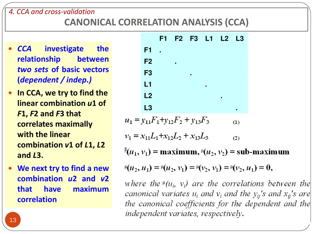
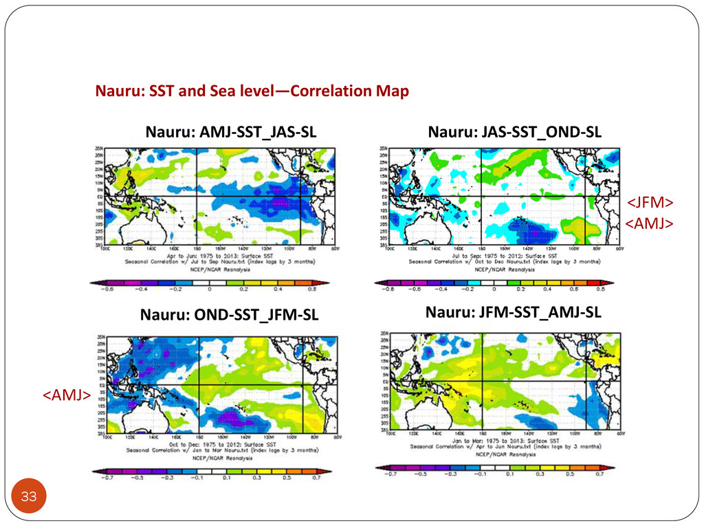
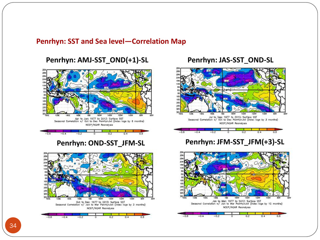
This presentation describes our seasonal sea level forecasting scheme. With a knowledge of current SST in the tropical ocean basins, and model predictions of how the oceans will likely evolve during the next several months, we use statistical model (CCA) to predict mean seasonal patterns of sea levels for 3-6 months in advance.

Rashed Chowdhury

July 31, 2013
Tweet

Other Decks in Research

Transcript

  1. 1 Climate Counts in the Pacific!! ‘Sea-level’ Variability and Predictability

    – USAPI Rashed Chowdhury Pacific ENSO Applications Climate Center University of Hawaii at Manoa, HI, USA What are we doing at PEAC? -- With a knowledge of current SST in the tropical ocean basins, and model predictions of how the oceans will likely evolve during the next several months, we use statistical model (CCA) to predict mean seasonal patterns of sea levels for 3-6 months in advance. 1. Introduction 2. Data and Methodology 3. Data analysis 4. CCA and Cross-Validation 5. CPT and Results 6. Non USAPI station
  2. SA SP LOCATION - USAPI REGION NIN O 3.4 Ni

    no 4 NWP Nino 3 ‘Hot Spots’ of Climate Hazards Seasonal Climate variability is correlated to ENSO 1. Introduction 2
  3. 3 Data Source (SL) JASL* Data Source (SST) NCEP/NCAR Data

    Processed at IRI Data Library Data Processed at UHSLC Entry to PEAC Data Base Quality control, Data check, Missing data adjustments Seasonality/ Harmonic Analysis SL, EN, LN Composites Scatterplots SST-SL SST /Wind Composites Corr. Map, SST-SL CCA/PCR Analysis ENSO-SLV Composites Yes/No No Yes Yes/No No Yes ENSO-SLV Correlation CPT/CCA X : Monthly SST Anomaly Y: Monthly SL Anomaly EOFs Cross-validated Skills /Forecasts EOFs D a t a p r e p a r a t i o n D a t a A n a l y s i s C C A a n d C P T Notes: *JASL is a collaborative effort of UHSLC, WDC-A, NODC, NCDD SL: Sea level; SST: Sea surface Temp; UHSLC: University of Hawaii Sea Level Center; IRI: International Rese. Inst. For Climate and Society; NCEP: National Center for Env. Prediction; NCAR: National Center for Atm. Research, EN: El Nino, LN: La Nina.; SLV: Sea level variability; CPT: Climate Predictability Tools; CCA: Canonical correlation Analysis; EOF: Empirical orthogonal functions. Reject Reject (3) (2) (1) 2. DATA/METHODOLOGY UHSLC http://ilikai.soest.hawaii.edu/uhslc/datai.html IRI Data Library: http://iridl.ldeo.columbia.edu/ SST/Wind Composites/Correlations: http://www.esrl.noaa.gov/psd/cgi- bin/data/composites/printpage.pl http://www.cdc.noaa.gov/Correlation/ CPT Software: http://iri.columbia.edu/outreach/software/)
  4. 4 1st harmonic Average (13.4N, 144.6E) (7.3N, 134.4E) (15.2N, 145.7E)

    (8.7N, 167.7E) (7.4N, 151.8E) (14.2S, 170.6W) (a) (b) (c) (d) (e) (f)
  5. -10 -5 0 5 10 Jul Aug Sep Oct Nov

    Dec Jan Feb Mar Apr May Jun Month SL deviations (inches) S_ElNino M_ElNino S_LaNina M_LaNina Guam Marshalls (Kwajalein) -10 -5 0 5 10 Jul Aug Sep Oct Nov Dec Jan Feb Mar Apr May Jun Month SL deviations (inches) S_ElNino M_ElNino S_LaNino M_LaNino 6 S El Niño: 1951, 58, 72, 82, & 97/ (Yr,0) S La Niña: 1964, 73, 75, 88, 98 (Yr, 0) M El Niño: 1963, 65, 69, 74, & 87 M La Niña: 1956, 70, 71, 84, 99 ENSO AND SEA LEVEL VARIABILITY Year (0) (+1) Year (0) (+1) Year (0) (+1) Composites of monthly Sea-level deviations in El Niño /La Niño years 3. Data Analysis
  6. 8 COMPOSITES OF STRONG El Niño and STRONG La Niña

    YEARS (SE-SL) –3 –1 0 +1 +2 EqC –E EqW-DL C-100S (e) (a) (c) (d) (f) (g) (h) (i) (b) (j) C-E Niño3.4
  7. LOWEST/HIGHEST SE LEVEL YEARS Lowest Highest GUAM 1967,72*,74,82*,97* 1971*,84*,96,98,99*,00 FSM

    1997,91,80,76,82 1984,99,00,75,01 CNMI 1997,86,83,95,90 1984,00,88,94,99 R PALAU 1997,91,80,72,76 1998,99,00,75,84 MARSHALLS 1982*,68,69*,72*,97* 2000,96,99*,98*,84* A SAMOA 1998,83*,58,78,53 1996,00,99,85,82 9 Strong El Niño years: 1951, 58, 72, 82, & 97/ Moderate El Niño years : 1963, 65, 69, 74, & 87 Strong La Niña years: 1964, 73, 75, 88, 98 Moderate La Niña years : 1956,70,71,84, 99
  8. SST COMPOSITES – LOW AND HIGH SEA LEVEL YEARS Guam

    El Niño signal La Niña signal 10
  9. 11 CORRELATION MAP – SST AND SEA LEVEL – 1

    Nino 3.4 NW-SW (13º48´N; 144º45´E) (09º0´N; 168º0´E) (14º2´S; 170º0´W) SC SC (a) (e) (c) (d) (b) (f)
  10. 12 Scatterplot sea-level and SST anomalies X-axis: sea-level deviations in

    mm; Y-axis: SST anomalies in deg. C. SCATTERPLOTS
  11. 13 CANONICAL CORRELATION ANALYSIS (CCA)  CCA investigate the relationship

    between two sets of basic vectors (dependent / indep.)  In CCA, we try to find the linear combination u1 of F1, F2 and F3 that correlates maximally with the linear combination v1 of L1, L2 and L3.  We next try to find a new combination u2 and v2 that have maximum correlation F1 F2 F3 L1 L2 L3 F1 . F2 . F3 . L1 . L2 . L3 . 4. CCA and cross-validation
  12. CCA CROSS-VALIDATION SKILLS 14  CCA: In CCA, we try

    to find the correlations between two data sets – dependent (Predictand) and independent (Predictor)  Cross Validation : A technique of repeatedly omitting a few observations from the data, reconstructing the model, and then making forecasts for the omitted cases. Cross validation is conducted to evaluate the overall forecasting skill of the CCA model  In our study, we remove only one observation at a time for each case. For example, to forecast the summer (JAS) ‘sea-level’ of 2013 with one-season lead, we take 38-yr JAS SL time series (1975–2012) and a 38-yr spring (AMJ) SST series to build the CCA model  Then this resulting CCA model is used to forecast ‘sea-level’ values in summer (JAS) 2013 using SST values in spring (AMJ) 2013.
  13. Choose the analysis to perform: PCR or CCA CPT -

    SELECTING THE ANALYSIS 5. CPT and Results 15
  14. 17  Input Datasets  CPT Input File Formats 

    Selecting Input Files  Setting the Training Periods  Setting Analysis Options  Missing values  Saving Program Settings  Running CPT  Data Analysis  Results : graphics (scree plots)  Results : EOF (Spatial and Temporal)  Results: Hindcasts  Indications of Uncertainty  Adjusting the Bootstrap Settings  Results : data files  Saving Output Files  Forecast CPT – AN OVERVIEW
  15. “X variables” or “X Predictors” dataset; (SST, monthly anomaly) (NCEP

    monthly SST field; NOAA NCDC ERSST version 3b sst) “Y variables” or “Y Predictands” dataset (SL, monthly deviations) (UHSLC) INPUT DATASETS 18
  16. You have to choose the number of EOFs for the

    predictor and predictand fields used to fit the model. If you set the minimum to be less than the maximum, CPT will find the optimum number of modes between the two numbers. However, if you set the minimum equal to the maximum, then CPT will use that number of modes. The number of CCA modes must also be set. SETTING ANALYSIS OPTIONS 19
  17. Optimizing the numbers of EOF and CCA modes: 1. CPT

    uses X and Y EOF #1 and CCA mode #1 to make cross- validated forecasts, then calculates a “goodness index” summarizing how good all the forecasts are (the closer to 1 the better). Then CPT uses Y EOFs #1 and #2 to remake cross- validated forecasts and calculates a new goodness index for these, and so on until using all possible combinations of modes. 2. At each step CPT compares the goodness indices and retains under the column “OPTIMUM” the highest goodness index and the corresponding number of modes (in the example above, 1, 1, 1). 3. CPT uses these number of modes to build the model. DATA ANALYSIS 20
  18. The menu Tools => Graphics => Scree plots displays the

    percentage of variance associated with each EOF plotted. RESULTS : graphics 21
  19. 22 Table: Percentage of variance explained by eigenvectors for the

    Pacific SSTs Ek/SST JFM SSTs AMJ SSTs JAS SSTs OND SSTs E1 E2 E3 E4 E5 E6 E7 E8 30.5 (30.5) 15.5 (46.0) 10.5 (56.5) 6.2 (62.7) 5.1 (67.8) 4.5 (72.3) 3.5 (75.8) 26.2 (26.2) 17.1 (43.3) 9.5 (52.8) 6.5 (59.3) 5.0 (64.3) 4.5 (68.7) 3.8 (72.5) 3.0 (75.5) 29.0 (29.0) 17.5 (46.5) 8.1 (54.6) 7.0 (61.6) 5.0 (66.6) 4.0 (70.6) 3.2 (73.8) 2.8 (76.0) 31.5 (31.5) 17.5 (49.0) 8.1 (57.1) 5.2 (62.3) 4.0 (66.3) 3.8 (70.1) 3.0 (73.1) (values in parentheses are cumulative variance by the k largest eigenvalues) Ek/SL JFM SL AMJ SL JAS SL OND SL E1 E2 E3 66.0 (66.0) 18.0 (84.0) 7.0 (91.0) 58.0 (58.0) 25.0 (83.0) 52.0 (52.0) 32.0 (84.0) 54.0 (54.0) 34.0 (88.0) 8.0 (96.0) Table : Percentage of variance explained by eigenvectors for sea levels
  20. 1. The menu Tools => Graphics => X EOF loadings

    and scores displays the loading pattern of each X EOF and the temporal series. 2. CPT allows you to customize and save each graphic by: right-clicking on the mouse selecting the graphic to customize / save RESULTS : graphics 23
  21. To see the series forecasted and observed at each station/grid

    go to: Tools => Validation => Cross-Validated => Performance Measures This menu displays some statistics of the forecast, such as correlation coefficient, RMSE, ROC etc (for more details refer to the help page). RESULTS: Cross validated skills 26
  22. The option Series shows the predicted values (cross) for the

    current station as well as forecast possibilities, confidence limits for the forecast and, in the “Thresholds” box, the “category thresholds” as well as the climatological probabilities for the 3 categories. Below Normal Above Normal Predicted Value FORECAST 27
  23. CCA CROSS-VALIDATION SKILLS 28 CCA Hindcast skills (left panel) and

    average skills at 0 to 3 seasons lead time (right panel). Note that 0, 1, 2, 3 represent zero, one, two, and three seasons lead time. For example, JFM-0, 1, 2, and means ‘sea-level’ of target season JFM based on SSTs of previous OND, JAS, AMJ, and JFM respectively. EOF (%) X:75.8 Y:91.0 X:75.5 Y:83.0 X:76.0 Y:84.0 X:73.1 Y:96.0
  24. PCR CROSS-VALIDATION SKILLS 29 PCR Hindcast skills (left panel) and

    average skills at 0 to 3 seasons lead time (right panel). Note that 0, 1, 2, 3 represent zero, one, two, and three seasons lead time. For example, JFM-0, 1, 2, and means ‘sea-level’ of target season JFM based on SSTs of previous OND, JAS, AMJ, and JFM respectively. EOF (%) X:75.8 Y:91.0 X:75.5 Y:83.0 X:76.0 Y:84.0 X:73.1 Y:96.0 0.3 0.6 0.9 0 1 2 3 0 1 2 3 0 1 2 3 0 1 2 3 JFM AMJ JAS OND Target Seasons PCR Cross Validation skill Guam Marshalls A Samoa 0.3 0.5 0.7 Lead (0) Lead (1) Lead (2) Lead (3) Leading seasons Average PCR skill Guam Marshalls A Samoa
  25. 30 -4.0 4.0 12.0 20.0 28.0 0.4 0.6 0.8 1

    Guam Malakal Yap Pohnpei Majuro Kwajalein Pago- Pago % of improvement C C A s k i l l SST SST+Wind % change SST and SST+Wind-based Sea-level forecasts – CCA cross-validation skill (0-season lead)
  26. 31 -4.0 4.0 12.0 20.0 28.0 0.4 0.6 0.8 1.0

    0 1 2 3 0 1 2 3 0 1 2 3 0 1 2 3 0 1 2 3 0 1 2 3 0 1 2 3 Guam Malakal Yap Pohnpei Majuro Kwajalein PagoPago % of improvement C C A s k i l l SST SST+U % of change SST and SST-Wind-based Sea-level forecasts – CCA cross-validation skill (0-3 season lead)
  27. Station Name Data Available Current stage of work Nauru Jan

    1975- Apr 2013 SST-SL Correlation map Honiara Jan 1975- Apr 2013 SST-SL Correlation map Funafuti Jan 1977 –Apr 2013 SST-SL Correlation map Suva Jan 1998 – Apr 2013 Missing 1975-1997 Penrhyn Jan 1977 – Oct 2012 SST-SL Correlation map Kanton Jan 1975 – Mar 2012 Missing 1980-83, 2001-03 Christmas Jan 1975 – Apr 2013 Data preparation Rarotong Jan 1977 – Apr 2013 Data preparation Papeete Jan 1975 – Apr 2013 Data preparation Rikita Jan 1975 – Apr 2013 Data preparation 32 ‘Sea-level’ Variability and Predictability – Non-USAPI 6. Non USAPI Stations
  28. 35 CONCLUSIONS (https://www.facebook.com/peaccenter) As an adaptation strategy, the ENSO-based sea

    level forecasts, warning, and response experience of PEAC can help other small island countries in the Pacific for longer time- scale climate variability and change. 100th Conference Call (March 7, 2013)