Upgrade to Pro — share decks privately, control downloads, hide ads and more …

A Few Thoughts on Characterizing Quantum Hardware

A Few Thoughts on Characterizing Quantum Hardware

A talk I gave to update my dissertation committee about my research. Released under SAND2017-12110 PE.

Travis Scholten

October 11, 2017
Tweet

More Decks by Travis Scholten

Other Decks in Science

Transcript

  1. Sandia National Laboratories is a multimission laboratory managed and operated

    by National Technology and Engineering Solutions of Sandia LLC, a wholly owned subsidiary of Honeywell International Inc. for the U.S. Department of Energy’s National Nuclear Security Administration under contract DE-NA0003525. CCR Center for Computing Research A Few Thoughts on Characterizing Quantum Hardware Travis L Scholten @Travis_Sch Center for Quantum Information and Control, UNM Center for Computing Research, Sandia National Laboratories
  2. MORE INFORMATION Full tomography (e.g., GST) Randomized benchmarking Crosstalk characterization

    Depending on how much information we want to learn, we have a plethora of techniques at our disposal… Generator tomography Robust phase estimation 58 MORE QUBITS
  3. …but each has some limits to its applicability and usefulness.

    Full tomography (e.g., GST) Randomized benchmarking Crosstalk characterization Generator tomography Robust phase estimation 57 MORE QUBITS MORE INFORMATION
  4. …but each has some limits to its applicability and usefulness.

    Full tomography (e.g., GST) Randomized benchmarking Crosstalk characterization Generator tomography Robust phase estimation How do we get more information out of more qubits? 56 MORE QUBITS MORE INFORMATION
  5. A brief review of what I’ve been thinking about: 2014

    Statistics Statistical Inference In Quantum Tomography - Uses of Hypothesis Testing and Information Criteria Travis L Scholten! University of New Mexico! Sandia National Labs! (Department 1425)! ! CQuIC Candidacy Exam @ UNM! 30 October 2014 1. Tomography! 2. Better Tomography! 3. Classical Hypothesis Testing! 4. Model Selection! 5. Results Sandia National Laboratories is a multi-program laboratory operated by Sandia Corporation, a wholly owned subsidiary of Lockheed Martin Corporation, for the U.S. Department of Energy’s National Nuclear Security Administration under contract DE-AC04-94AL85000. 0/55 Use model selection to choose simpler, yet justifiable, models. Quantum Information 55
  6. A brief review of what I’ve been thinking about: 2015

    How do boundaries affect model selection? ON THE EDGE:! STATE TOMOGRAPHY, BOUNDARIES,! AND MODEL SELECTION Travis L Scholten! Center for Computing Research! Sandia National Labs CQuIC Talk! University of New Mexico! 2015 December 2 Sandia National Laboratories is a multi-program laboratory managed and operated by Sandia Corporation, a wholly owned subsidiary of Lockheed Martin Corporation, for the U.S. Department of Energy’s National Nuclear Security Administration under contract DE-AC04-94AL85000. CCR Center for Computing Research 59 Geometry Statistics Quantum Information 54
  7. A brief review of what I’ve been thinking about: 2016

    Quantum Information Statistics Just how much information do we need to learn, anyway? An Effective State Space Dimension For A Quantum System Travis L Scholten @Travis_Sch Center for Quantum Information and Control University of New Mexico Center for Computing Research Sandia National Labs, New Mexico Sandia National Laboratories is a multi-mission laboratory managed and operated by Sandia Corporation, a wholly owned subsidiary of Lockheed Martin Corporation, for the U.S. Department of Energy’s National Nuclear Security Administration under contract DE-AC04-94AL85000. CCR Center for Computing Research Geometry Compressed Sensing 53
  8. A brief review of what I’ve been thinking about: 2017

    Quantum Information Statistics Compressed Sensing Geometry Machine Learning How can machine learning extract useful information? 52 Sandia National Laboratories is a multimission laboratory managed and operated by National Technology and Engineering Solutions of Sandia LLC, a wholly owned subsidiary of Honeywell International Inc. for the U.S. Department of Energy’s National Nuclear Security Administration under contract DE-NA0003525. CCR Center for Computing Research A Few Thoughts on Characterizing Quantum Hardware Travis L Scholten @Travis_Sch Center for Quantum Information and Control, UNM Center for Computing Research, Sandia National Laboratories
  9. Behavior of the Maximum Likelihood in Quantum State Tomography Travis

    L Scholten and Robin Blume-Kohout Center for Computing Research (CCR), Sandia National Labs and Center for Quantum Information and Control (CQuIC), University of New Mexico (Dated: August 18, 2017) Quantum state tomography on a d-dimensional system demands resources that grow rapidly with d. They may be reduced by using model selection to tailor the number of parameters in the model (i.e., the size of the density matrix). Most model selection methods typically rely on a test statistic and a null theory that describes its behavior when two models are equally good. Here, we consider the loglikelihood ratio. Because of the positivity constraint ⇢ 0, quantum state space does not generally satisfy local asymptotic normality, meaning the classical null theory for the loglikelihood ratio (the Wilks theorem) should not be used. Thus, understanding and quantifying how positivity a↵ects the null behavior of this test statistic is necessary for its use in model selection for state tomography. We define a new generalization of local asymptotic normality, metric-projected local asymptotic normality, show that quantum state space satisfies it, and derive a replacement for the Wilks theorem. In addition to enabling reliable model selection, our results shed more light on the qualitative e↵ects of the positivity constraint on state tomography. Determining the quantum state ⇢ 0 produced by a spe- cific preparation procedure for a quantum system is a problem almost as old as quantum mechanics itself [1, 2]. This task, known as quantum state tomography [3], is not only useful in its own right (diagnosing and detect- We’ll be discussing a paper and some exploratory machine learning work. arXiv:1609.04385 (v2: 2017 August) Dimensionality reduction Support vector machines 51
  10. Behavior of the Maximum Likelihood in Quantum State Tomography Travis

    L Scholten and Robin Blume-Kohout Center for Computing Research (CCR), Sandia National Labs and Center for Quantum Information and Control (CQuIC), University of New Mexico (Dated: August 18, 2017) Quantum state tomography on a d-dimensional system demands resources that grow rapidly with d. They may be reduced by using model selection to tailor the number of parameters in the model (i.e., the size of the density matrix). Most model selection methods typically rely on a test statistic and a null theory that describes its behavior when two models are equally good. Here, we consider the loglikelihood ratio. Because of the positivity constraint ⇢ 0, quantum state space does not generally satisfy local asymptotic normality, meaning the classical null theory for the loglikelihood ratio (the Wilks theorem) should not be used. Thus, understanding and quantifying how positivity a↵ects the null behavior of this test statistic is necessary for its use in model selection for state tomography. We define a new generalization of local asymptotic normality, metric-projected local asymptotic normality, show that quantum state space satisfies it, and derive a replacement for the Wilks theorem. In addition to enabling reliable model selection, our results shed more light on the qualitative e↵ects of the positivity constraint on state tomography. ermining the quantum state ⇢ 0 produced by a spe- preparation procedure for a quantum system is a em almost as old as quantum mechanics itself [1, 2]. task, known as quantum state tomography [3], is nly useful in its own right (diagnosing and detect- rors in state preparation), but is also used in other cterization protocols including entanglement verifi- [4–6] and process tomography [7]. A typical state Quantum state space has boundaries. They affect the behavior of tomographic techniques. arXiv:1609.04385 (v2: 2017 August) 50
  11. Quantum state space has boundaries, posing some challenges for tomography

    & model selection. ⇢ 0 ⇢ 0 ⇢ 0 ⇢ 0 Tomography: Boundaries distort the distribution of maximum likelihood estimates (makes reasoning about their properties hard). Model selection: Common techniques (Wilks theorem, information criteria) cannot be used! Easy to reason about (many known results) Hard to reason about (known results don’t apply!) 49
  12. In classical statistics, models often satisfy local asymptotic normality (LAN).

    If LAN is satisfied, then asymptotically: Likelihoods are Gaussian: (Here, model = set of density matrices.) L ( ⇢ ) ⌘ Pr(Data |⇢ ) / N!1 Exp  1 2 Tr( ⇢ ˆ ⇢ML,M) F ( ⇢ ˆ ⇢ML,M) 48
  13. In classical statistics, models often satisfy local asymptotic normality (LAN).

    If LAN is satisfied, then asymptotically: Maximum likelihood (ML) estimates are normally distributed: (Here, model = set of density matrices.) ˆ ⇢ML,M ⌘ argmax ⇢2M L ( ⇢ ) d ! N ( ⇢0, F 1 ) (M = R2) ⇢0 47
  14. Because models used in tomography have boundaries, local asymptotic normality

    (LAN) is generally violated. Consequences of violation of LAN: Likelihoods are not Gaussian: Maximum likelihood (ML) estimates are not normally distributed: (M = {( x, y ) 2 R2 | x 2 + y 2  1}) L ( ⇢ ) ⌘ Pr(Data |⇢ ) / N!1 Exp  1 2 Tr( ⇢ ˆ ⇢ML,M) F ( ⇢ ˆ ⇢ML,M) ˆ ⇢ML,M ⌘ argmax ⇢2M L ( ⇢ ) d ! N ( ⇢0, F 1 ) (Here, model = set of density matrices.) 46 ⇢0
  15. Behavior of the Maximum Likelihood in Quantum State Tomography Travis

    L Scholten and Robin Blume-Kohout Center for Computing Research (CCR), Sandia National Labs and Center for Quantum Information and Control (CQuIC), University of New Mexico (Dated: August 18, 2017) Quantum state tomography on a d-dimensional system demands resources that grow rapidly with d. They may be reduced by using model selection to tailor the number of parameters in the model (i.e., the size of the density matrix). Most model selection methods typically rely on a test statistic and a null theory that describes its behavior when two models are equally good. Here, we consider the loglikelihood ratio. Because of the positivity constraint ⇢ 0, quantum state space does not generally satisfy local asymptotic normality, meaning the classical null theory for the loglikelihood ratio (the Wilks theorem) should not be used. Thus, understanding and quantifying how positivity a↵ects the null behavior of this test statistic is necessary for its use in model selection for state tomography. We define a new generalization of local asymptotic normality, metric-projected local asymptotic normality, show that quantum state space satisfies it, and derive a replacement for the Wilks theorem. In addition to enabling reliable model selection, our results shed more light on the qualitative e↵ects of the positivity constraint on state tomography. ermining the quantum state ⇢ 0 produced by a spe- preparation procedure for a quantum system is a em almost as old as quantum mechanics itself [1, 2]. task, known as quantum state tomography [3], is Show how to generalize LAN for models with convex boundaries. Provide a replacement for the Wilks Theorem We: arXiv:1609.04385 (v2: 2017 August) 45
  16. To generalize LAN for models with convex boundaries, we embed

    them inside larger models. In state tomography, (lift trace and positivity constraints) M = {⇢ 2 B(H) | ⇢ = ⇢†, Tr(⇢) = 1, ⇢ 0} (all density matrices) M0 = { 2 B(H) | = †} M0 44 M
  17. If the larger model satisfies LAN, we can prove properties

    of the restricted model. A. Definitions and Overview of Results The main definitions and results required for the re- mainder of the paper are presented in this subsection. Technical details and proofs are presented in the next subsection. Definition 1 (Metric-projected local asymptotic nor- mality, or MP-LAN) . A model M satisfies MP-LAN if, and only if, M is a convex subset of a model M0 that satisfies LAN. Although the definition of MP-LAN is rather short, it implies some very useful properties. These properties follow from the fact that, as N ! 1, the behavior of ˆ ⇢ ML,M and is entirely determined by their behavior in an arbitrarily small region of M around ⇢ 0 , which we call the local state space. satisfies LAN satisfies “MP-LAN” 43 M0 M
  18. Through this embedding, each ML estimate in the restricted model

    is related to one in the larger. ˆ ⇢ML,M0 ⇠ N(⇢0, F 1) L ( ⇢ ) / Exp ⇥ 1 2 Tr( ⇢ ˆ ⇢ML,M0 ) F ( ⇢ ˆ ⇢ML,M0 ) ⇤ Because M0 satisfies LAN: 42 M M0
  19. =) ˆ ⇢ML,M = argmin ⇢2M Tr[(⇢ ˆ ⇢ML,M0 )F(⇢

    ˆ ⇢ML,M0 )] ML estimate in restricted model is the “metric projection” of the ML estimate in the larger model. Through this embedding, each ML estimate in the restricted model is related to one in the larger. 41 M M0 L ( ⇢ ) / Exp ⇥ 1 2 Tr( ⇢ ˆ ⇢ML,M0 ) F ( ⇢ ˆ ⇢ML,M0 ) ⇤ Because M0 satisfies LAN:
  20. Behavior of the Maximum Likelihood in Quantum State Tomography Travis

    L Scholten and Robin Blume-Kohout Center for Computing Research (CCR), Sandia National Labs and Center for Quantum Information and Control (CQuIC), University of New Mexico (Dated: August 18, 2017) Quantum state tomography on a d-dimensional system demands resources that grow rapidly with d. They may be reduced by using model selection to tailor the number of parameters in the model (i.e., the size of the density matrix). Most model selection methods typically rely on a test statistic and a null theory that describes its behavior when two models are equally good. Here, we consider the loglikelihood ratio. Because of the positivity constraint ⇢ 0, quantum state space does not generally satisfy local asymptotic normality, meaning the classical null theory for the loglikelihood ratio (the Wilks theorem) should not be used. Thus, understanding and quantifying how positivity a↵ects the null behavior of this test statistic is necessary for its use in model selection for state tomography. We define a new generalization of local asymptotic normality, metric-projected local asymptotic normality, show that quantum state space satisfies it, and derive a replacement for the Wilks theorem. In addition to enabling reliable model selection, our results shed more light on the qualitative e↵ects of the positivity constraint on state tomography. ermining the quantum state ⇢ 0 produced by a spe- preparation procedure for a quantum system is a em almost as old as quantum mechanics itself [1, 2]. task, known as quantum state tomography [3], is Show how to generalize LAN for models with convex boundaries. We: Provide a replacement for the Wilks Theorem arXiv:1609.04385 (v2: 2017 August) 40
  21. The Wilks Theorem describes the behavior of the loglikelihood ratio

    statistic. The loglikelihood ratio statistic is defined as “How much better does the ML estimate fit the data than the truth itself?” (In order to compare two models, sufficient to answer this question for both.) ( ⇢0, M ) = 2 log ✓ L ( ⇢0) L (ˆ ⇢ML,M) ◆ ! LAN Tr[( ⇢0 ˆ ⇢ML,M0 ) F ( ⇢0 ˆ ⇢ Tr[(ˆ ⇢ML,M ˆ ⇢ML,M0 ) F = PT Tr[( ⇢0 ˆ ⇢ML,M) F ( ⇢0 ˆ ⇢M ⇠ stats 2 dim(M) 39
  22. If the model satisfies LAN & contains the true state

    M = R2 M0 = R3 ( ⇢0, M ) = 2 log ✓ L ( ⇢0) L (ˆ ⇢ML,M) ◆ ! LAN Tr[( ⇢0 ˆ ⇢ML,M0 ) F ( ⇢0 ˆ ⇢ML,M0 )] Tr[(ˆ ⇢ML,M ˆ ⇢ML,M0 ) F (ˆ ⇢ML,M ˆ ⇢ML,M0 )] = PT Tr[( ⇢0 ˆ ⇢ML,M) F ( ⇢0 ˆ ⇢ML,M)] ⇠ stats 2 dim(M) The Wilks Theorem describes the behavior of the loglikelihood ratio statistic. 38
  23. If the model satisfies LAN & contains the true state

    then, asymptotically, M = R2 M0 = R3 ( ⇢0, M ) = 2 log ✓ L ( ⇢0) L (ˆ ⇢ML,M) ◆ ! LAN Tr[( ⇢0 ˆ ⇢ML,M0 ) F ( ⇢0 ˆ ⇢ML,M0 )] Tr[(ˆ ⇢ML,M ˆ ⇢ML,M0 ) F (ˆ ⇢ML,M ˆ ⇢ML,M0 )] = PT Tr[( ⇢0 ˆ ⇢ML,M) F ( ⇢0 ˆ ⇢ML,M)] ⇠ stats 2 dim(M) The Wilks Theorem describes the behavior of the loglikelihood ratio statistic. 37
  24. If the model satisfies LAN & contains the true state

    then, asymptotically, M = R2 M0 = R3 ( ⇢0, M ) = 2 log ✓ L ( ⇢0) L (ˆ ⇢ML,M) ◆ ! LAN Tr[( ⇢0 ˆ ⇢ML,M0 ) F ( ⇢0 ˆ ⇢ML,M0 )] Tr[(ˆ ⇢ML,M ˆ ⇢ML,M0 ) F (ˆ ⇢ML,M ˆ ⇢ML,M0 )] = PT Tr[( ⇢0 ˆ ⇢ML,M) F ( ⇢0 ˆ ⇢ML,M)] ⇠ stats 2 dim(M) (requires isotropic Fisher information, or that models are vector spaces) The Wilks Theorem describes the behavior of the loglikelihood ratio statistic. 36
  25. Defining a particular set of models, the Wilks Theorem fails

    spectacularly. 5 10 15 20 25 30 d (Hilbert Space Dimension) 0 200 400 600 800 h (⇢0 , Md )i Wilks Theorem Rank(⇢0 ) =10 (various colors) Rank(⇢0 ) = 2...9 Rank(⇢0 ) =1 Md = {⇢ 2 B(Hd) | Tr(⇢) = 1, ⇢ 0} h (⇢0, Md)i = d2 1 Wilks Theorem says Define (d-dimensional density matrices) 35
  26. M = R2 M0 = R3 ( ⇢0, M )

    = 2 log ✓ L ( ⇢0) L (ˆ ⇢ML,M) ◆ ! LAN Tr[( ⇢0 ˆ ⇢ML,M0 ) F ( ⇢0 ˆ ⇢ML,M0 )] Tr[(ˆ ⇢ML,M ˆ ⇢ML,M0 ) F (ˆ ⇢ML,M ˆ ⇢ML,M0 )] = PT Tr[( ⇢0 ˆ ⇢ML,M) F ( ⇢0 ˆ ⇢ML,M)] ⇠ stats 2 dim(M) (requires isotropic Fisher information, or that models are vector spaces) The Wilks Theorem describes the behavior of the loglikelihood ratio statistic. If the model satisfies LAN & contains the true state then, asymptotically, 34 Quantum state space doesn’t satisfy LAN, so Wilks won’t apply… let’s find something that does!
  27. Quantum state space does satisfy MP-LAN. This lets us derive

    a replacement for Wilks. Md = {⇢ 2 B(Hd) | Tr(⇢) = 1, ⇢ 0} Define 33 Md
  28. M0 d Md = {⇢ 2 B(Hd) | Tr(⇢) =

    1, ⇢ 0} Define This model satisfies MP-LAN, using Quantum state space does satisfy MP-LAN. This lets us derive a replacement for Wilks. M0 d = { | dim( ) = d, = †} Md 32
  29. Md = {⇢ 2 B(Hd) | Tr(⇢) = 1, ⇢

    0} Define Because satisfies LAN, M0 d Quantum state space does satisfy MP-LAN. This lets us derive a replacement for Wilks. M0 d ( ⇢0, Md) = 2 log ✓ L ( ⇢0) L (ˆ ⇢ML,Md ) ◆ ! LAN Tr[( ⇢0 ˆ ⇢ML,M0 d ) F ( ⇢0 ˆ ⇢ML,M0 d )] Tr[(ˆ ⇢ML,Md ˆ ⇢ML,M0 d ) F ((ˆ ⇢ML,Md ˆ ⇢ML,M0 d )] = PT Tr[( ⇢0 ˆ ⇢ML,Md ) F (( ⇢0 ˆ ⇢ML,Md )] 31 Md
  30. Md = {⇢ 2 B(Hd) | Tr(⇢) = 1, ⇢

    0} Define Because the local state space is the tangent cone… Quantum state space does satisfy MP-LAN. This lets us derive a replacement for Wilks. ( ⇢0, M ) = 2 log ✓ L ( ⇢0) L (ˆ ⇢ML,M) ◆ ! LAN Tr[( ⇢0 ˆ ⇢ML,M0 ) F ( ⇢0 ˆ ⇢ML,M0 )] Tr[(ˆ ⇢ML,M ˆ ⇢ML,M0 ) F (ˆ ⇢ML,M ˆ ⇢ML,M0 )] = PT Tr[( ⇢0 ˆ ⇢ML,M) F ( ⇢0 ˆ ⇢ML,M)] ⇠ stats 2 dim(M) Because satisfies LAN, M0 d (Also useful for defining “quantum information criterion”) M0 d ( ⇢0, Md) = 2 log ✓ L ( ⇢0) L (ˆ ⇢ML,Md ) ◆ ! LAN Tr[( ⇢0 ˆ ⇢ML,M0 d ) F ( ⇢0 ˆ ⇢ML,M0 d )] Tr[(ˆ ⇢ML,Md ˆ ⇢ML,M0 d ) F ((ˆ ⇢ML,Md ˆ ⇢ML,M0 d )] = PT Tr[( ⇢0 ˆ ⇢ML,Md ) F (( ⇢0 ˆ ⇢ML,Md )] Md (⇢0, Md) 30 Md
  31. Our replacement for Wilks approximates the expected value of the

    loglikelihood ratio statistic. (⇢0, Md) = Tr[(⇢0 ˆ ⇢ML,Md )F(⇢0 ˆ ⇢ML,Md )] h (⇢0, Md)i = ?? 29
  32. To make progress, we assume the Fisher information is isotropic.

    (Never actually happens…except in trivial cases) 28 (⇢0, Md) = Tr[(⇢0 ˆ ⇢ML,Md )F(⇢0 ˆ ⇢ML,Md )] h (⇢0, Md)i = ?? Our replacement for Wilks approximates the expected value of the loglikelihood ratio statistic.
  33. 7 3. Expression for (⇢0, M) The loglikelihood ratio statistic

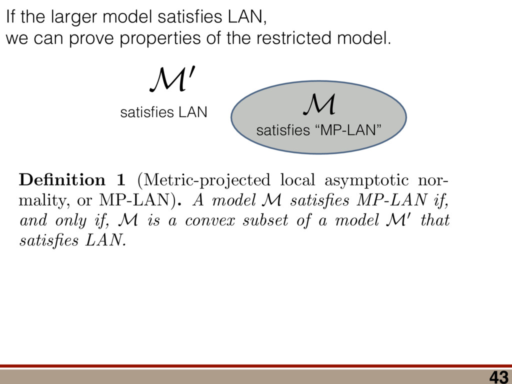
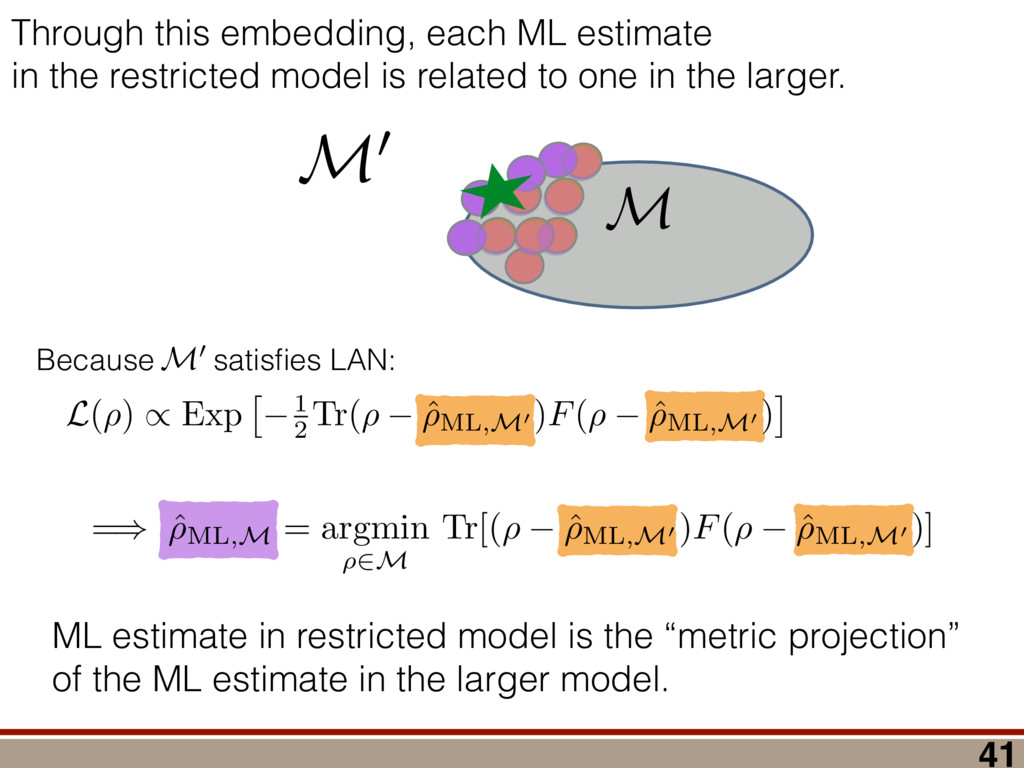
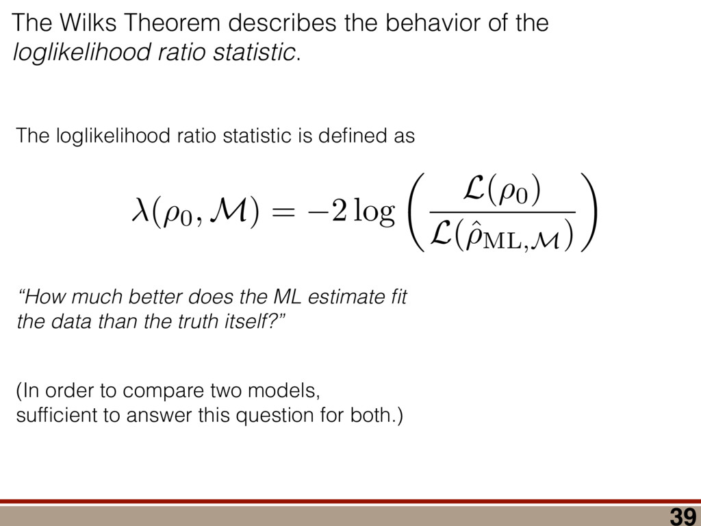
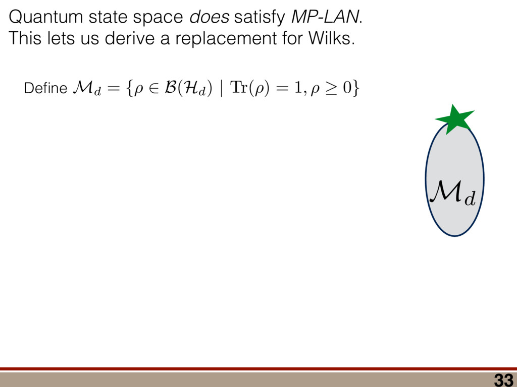
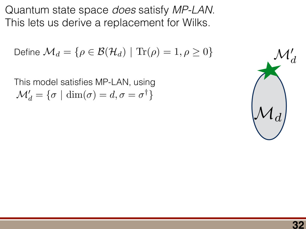
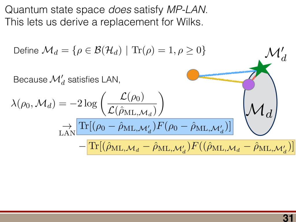
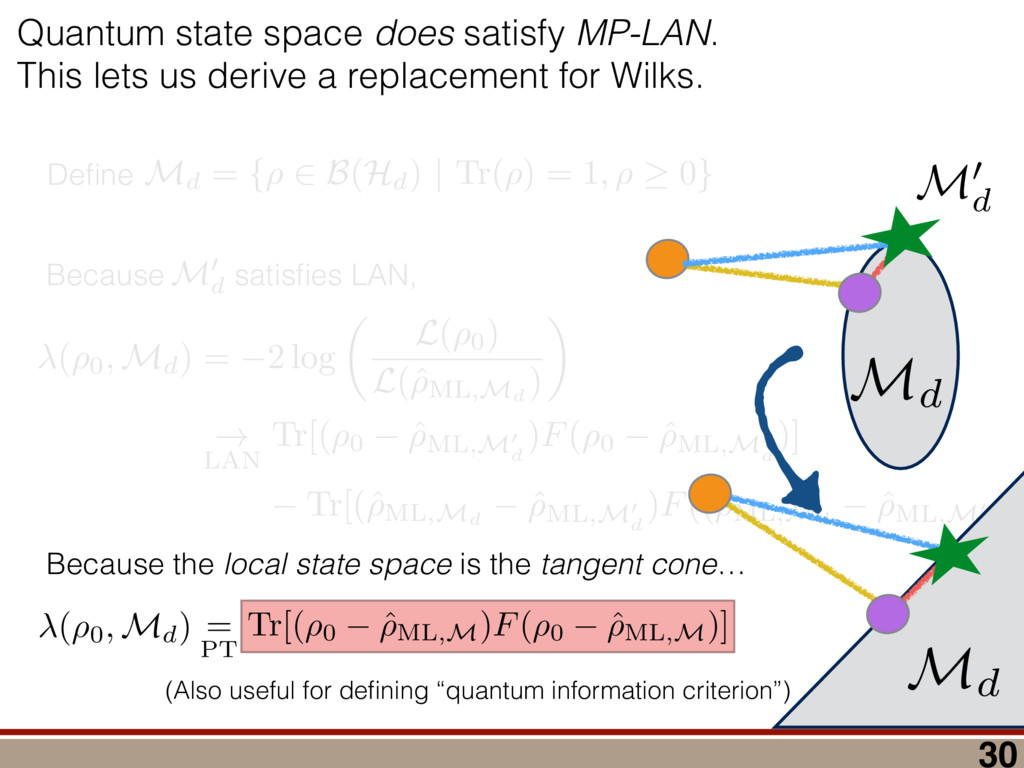
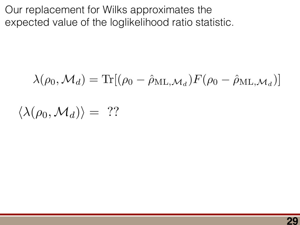
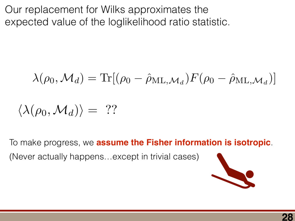
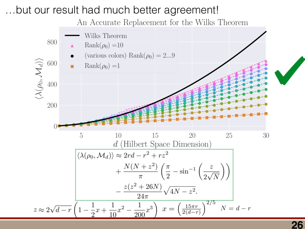
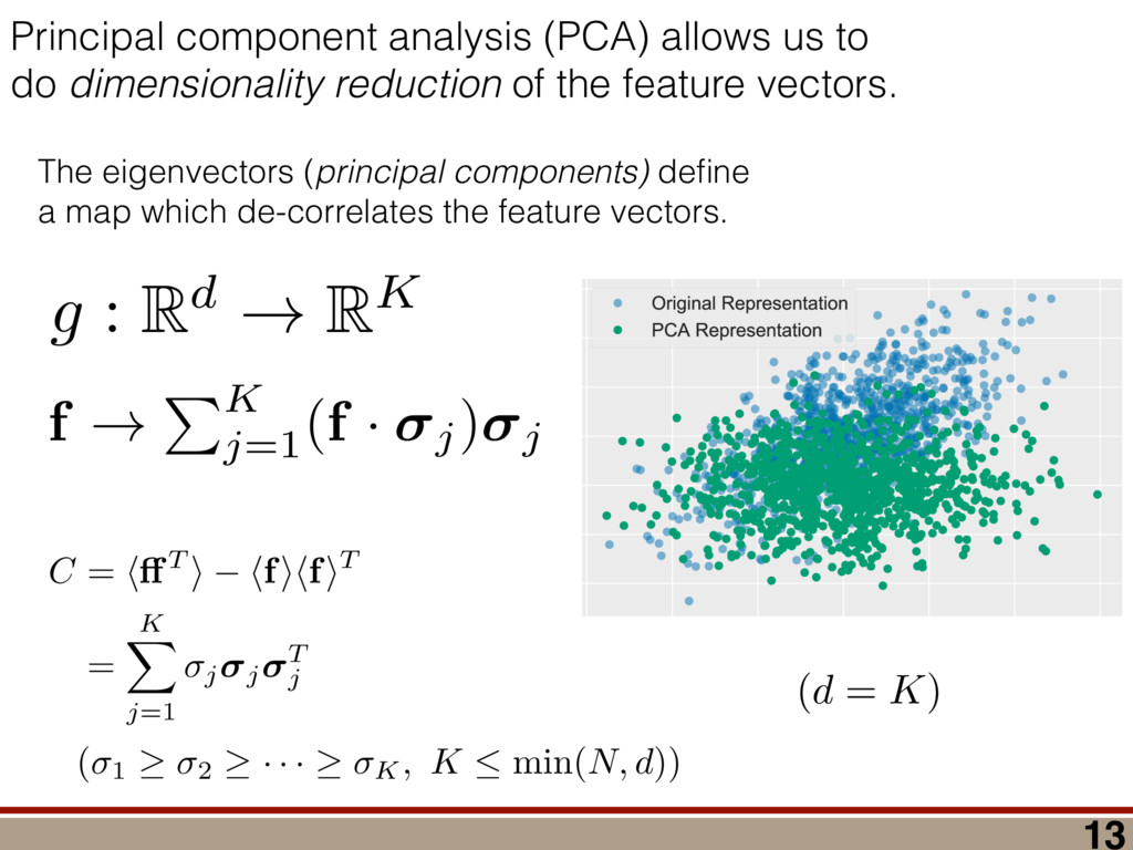
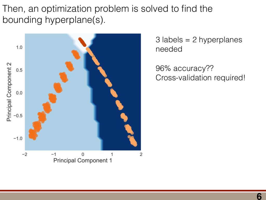
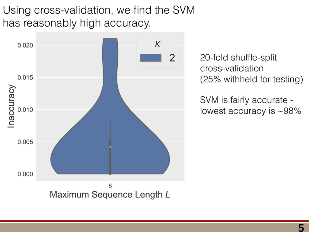
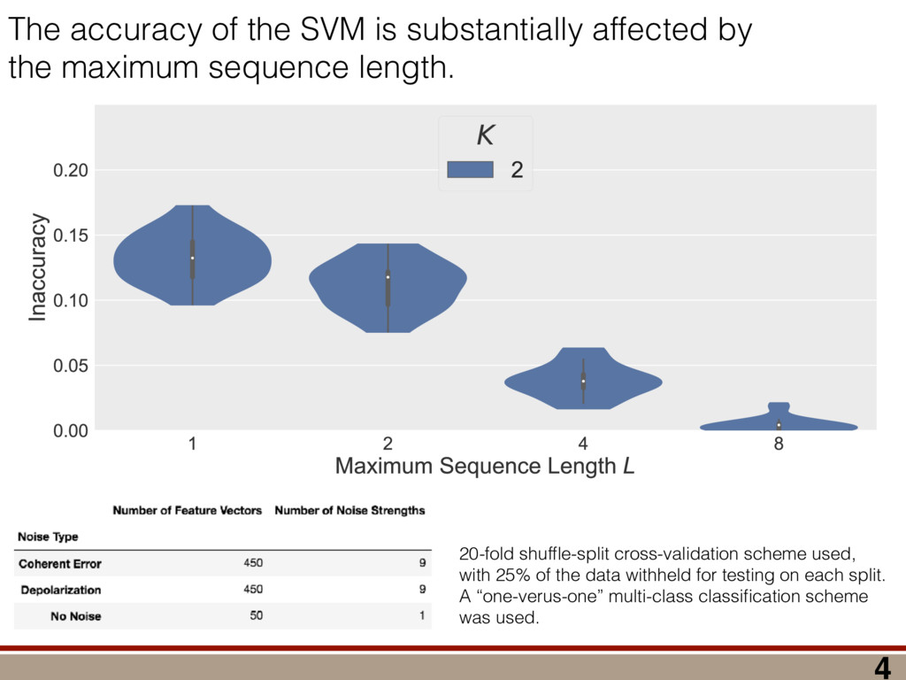
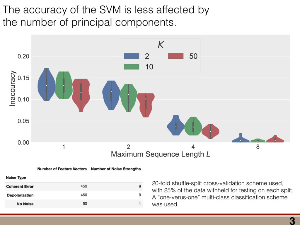
    between any two mod- els (M 1 , M 2 ) can be computed using a reference model R: (M 1 , M 2 ) = (R, M 2 ) (R, M 1 ), where (R, M) = 2 log ✓ L(R) L(M) ◆ = 2 log 0 @ max ⇢2R L(⇢) max ⇢2M L(⇢) 1 A . Let us take R = ⇢ 0 . Because as N ! 1 the likelihood L(⇢) is Gaussian around ˆ ⇢ ML,M0 , we have (⇢ 0 , M) = 2 log 0 @ L(⇢ 0 ) max ⇢2M L(⇢) 1 A ! N!1 Tr[(⇢ 0 ˆ ⇢ ML,M0 )I(⇢ 0 ˆ ⇢ ML,M0 )] Tr[(ˆ ⇢ ML,M ˆ ⇢ ML,M0 )I(ˆ ⇢ ML,M ˆ ⇢ ML,M0 )]. (9) Using the fact ˆ ⇢ ML,M is a metric projection, we can prove that (⇢ 0 , M) has a simple form. Lemma 4. (⇢ 0 , M) = Tr[(⇢ 0 ˆ ⇢ ML,M )I(⇢ 0 ˆ ⇢ ML,M )]. Proof. We switch to Fisher-adjusted coordinates (⇢ ! I1 / 2 ⇢), and in these coordinates I becomes 1l: (⇢ 0 , M) = Tr[(⇢ 0 ˆ ⇢ ML,M0 )2] Tr[(ˆ ⇢ ML,M ˆ ⇢ ML,M0 )2]. (10) To prove the lemma, we must consider two cases: Case 1: Assume ˆ ⇢ ML,M0 62 T(⇢ 0 ). Because ˆ ⇢ ML,M is the metric projection of ˆ ⇢ ML,M0 onto T(⇢ 0 ) (Equation (8)), the line joining ˆ ⇢ ML,M0 and ˆ ⇢ ML,M is normal to T(⇢ 0 ) at ˆ ⇢ ML,M . Because T(⇢ 0 ) contains ⇢ 0 (as its origin), it fol- lows that the lines joining ⇢ 0 to ˆ ⇢ ML,M , and ˆ ⇢ ML,M to ˆ ⇢ ML,M0 , are perpendicular. (See Figure 4.) By the Pythagorean theorem, we have Tr[(⇢ 0 ˆ ⇢ ML,M0 )2] = Tr[(⇢ 0 ˆ ⇢ ML,M )2]+Tr[(ˆ ⇢ ML,M ˆ ⇢ ML,M0 )2] Subtracting Tr[(ˆ ⇢ ML,M ˆ ⇢ ML,M0 )2] from both sides, and comparing to Equation (10), yields the lemma statement in Fisher-adjusted coordinates. Case 2: Assume ˆ ⇢ ML,M0 2 T(⇢ 0 ). Then, ˆ ⇢ ML,M = ˆ ⇢ ML,M0 , and Equation (10) simplifies to the lemma state- ment in Fisher-adjusted coordinates. Switching back from Fisher-adjusted coordinates, we have (⇢ 0 , M) = Tr[(⇢ 0 ˆ ⇢ ML,M )I(⇢ 0 ˆ ⇢ ML,M )]. So if M satisfies MP-LAN then as N ! 1 the log- likelihood ratio statistic becomes related to squared er- ror/loss (as measured by the Fisher metric.) This result may be of independent interest in, for example, defining new information criteria, which attempt to balance good- ness of fit (as measured by ) against error/loss (gener- ally, as measured by squared error). With these technical results in hand, we can proceed to compute h (Md , Md +1 )i in the next section. IV. A WILKS THEOREM FOR QUANTUM STATE SPACE To derive a replacement for the Wilks theorem, we start by showing the models Md satisfy MP-LAN. Lemma 5. The models Md , defined in Equation (4), satisfy MP-LAN. Proof. Let M0 d = { | dim( ) = d, = †}. (That is, M0 d is the set of all d ⇥ d Hermitian matrices, but we do not require them to be non-negative, nor trace-1.) It is clear Md ⇢ M0 d . Now, 8 2 M0 d , the likelihood L( ) is twice continuously di↵erentiable, meaning M0 d satisfies LAN. Thus, Md satisfies MP-LAN. We can reduce the problem of computing (Md , Md +1 ) to that of computing (⇢ 0 , Mk) for k = d, d + 1 using the identity (Md , Md +1 ) = (⇢ 0 , Md +1 ) (⇢ 0 , Md). where (⇢ 0 , Mk) is given in Equation (6). Because each model satisfies MP-LAN, asymptotically, (⇢ 0 , Mk) takes a very simple form, via Equation (7): (⇢ 0 , Mk) = Tr[(⇢ 0 ˆ ⇢ ML,Mk )Ik(⇢ 0 ˆ ⇢ ML,Mk )]. The Fisher information Ik is generally anisotropic, de- pending on ⇢ 0 , the POVM being measured, and the model Mk (see Figure 5). And while the ⇢ 0 con- straint that invalidated LAN in the first place is at least somewhat tractable in standard (Hilbert-Schmidt) co- ordinates, it becomes completely intractable in Fisher- adjusted coordinates. So, to obtain a semi-analytic null theory for , we will simplify to the case where Ik = 1lk /✏2 for some ✏ that scales as 1/ p N samples . (That is, Ik is proportional to the Hilbert-Schmidt metric.) This simplification permits the derivation of analytic results that capture realistic tomographic scenarios surprisingly well [51]. With this simplification, (Md , Md +1 ) is given by = 1 ✏2 Tr[(⇢ 0 ˆ ⇢ ML,d+1 )2] Tr[(⇢ 0 ˆ ⇢ ML,d )2] . (11) That is, is a di↵erence in Hilbert-Schmidt distances. This expression makes it clear why a null theory for is necessary: if ⇢ 0 2 Md , Md +1 , ˆ ⇢ ML,d+1 will lie further from ⇢ 0 than ˆ ⇢ ML,d (because there are more parameters that can fit noise in the data). The null theory for tells us how much extra error will be incurred in using Md +1 to reconstruct ⇢ 0 when Md is just as good. Describing Pr( ) is di cult because the distributions of ˆ ⇢ ML,d , ˆ ⇢ ML,d+1 are complicated, highly non-Gaussian, and singular (estimates “pile up” on the various faces of the boundary as shown in Figure 1). For this reason, we will not attempt to compute Pr( ) directly. Instead, we focus on deriving a good approximation for h i. We consider each of the terms in Equation (11) separately and focus on computing ✏2 h (⇢ 0 , Md)i = hTr[(ˆ ⇢ ML,d ⇢ 0 )2]i for arbitrary d. Doing so involves two main steps: 8 1.0 0.5 0.0 0.5 1.0 h X i 1.0 0.5 0.0 0.5 1.0 h Z i Anisotropic Fisher information (Rebit) FIG. 5. Anisotropy of the Fisher information for a rebit: Suppose a rebit state ⇢0 (star) is measured using the POVM 1 2 {|0ih0|, |1ih1|, |+ih+|, | ih |}. Depending on ⇢0 , the distribution of the unconstrained estimates ˆ ⇢ML (ellipses) may be anisotropic. Imposing the positivity constraint ⇢ 0 is di cult in Fisher-adjusted coordinates; in this paper, we simplify these complexities to the case where I / 1l, and is independent of ⇢0 . (1) Identify which degrees of freedom in ˆ ⇢ ML,M0 d are, and are not, a↵ected by projection onto the tangent cone T(⇢ 0 ). (2) For each of those categories, evaluate its contribu- tion to the value of h i. In Section IV A, we identify two types of degrees of freedom in ˆ ⇢ ML,M0 , which we call the “L” and the “kite”. Section IV B computes the contribution of degrees of free- dom in the “L”, and Section IV C computes the contri- bution from the “kite”. The total expected value is given in Equation (19) in Section IV D, on page 11. A. Separating out Degrees of Freedom in ˆ ⇢ML,M0 d We begin by observing that (⇢ 0 , Md) can be written as a sum over matrix elements, = ✏ 2Tr[(ˆ ⇢ ML,d ⇢ 0 )2] = ✏ 2 X jk |(ˆ ⇢ ML,d ⇢ 0 )jk |2 = X jk jk where jk = ✏ 2|(ˆ ⇢ ML,d ⇢ 0 )jk |2, and therefore h i = P jk h jk i. Each term h jk i quan- tifies the mean-squared error of a single matrix element of ˆ ⇢ ML,d , and while the Wilks theorem predicts h jk i = 1 for all j, k, due to positivity constraints, this no longer holds. In particular, the matrix elements of ˆ ⇢ ML,d now fall into two parts: 1. Those for which the positivity constraint does a↵ect their behavior. “Kite” “L” “L” Matrix Elements of ˆM d 1 0.98 0.12 0.12 0.12 0.11 0.11 0.3 1 1 0.12 0.12 0.11 0.12 0.33 0.11 1 1 0.12 0.12 0.12 0.34 0.12 0.11 1 1 0.12 0.12 0.29 0.12 0.11 0.12 0.99 0.99 0.13 0.38 0.12 0.12 0.12 0.12 0.94 1 0.35 0.13 0.12 0.12 0.12 0.12 1 2.6 1 0.99 1 1 1 0.98 2.7 1 0.94 0.99 1 1 1 1 h jk i FIG. 6. Division of the matrix elements of ˆ ⇢ML,M0 d : When a rank-2 state is reconstructed in d = 8 dimensions, the total loglikelihood ratio (⇢0, M8 ) is the sum of terms jk from errors in each matrix element (ˆ ⇢ML,d )jk . Left: Numerics show a clear division; some matrix elements have h jk i ⇠ 1 as predicted by the Wilks theorem, while others are either more or less. Right: The numerical results support our theoretical reasoning for dividing the matrix elements of ˆ ⇢ML,M0 d into two parts: the “kite” and the “L”. 2. Those for which the positivity constraint does not a↵ect their behavior, as they correspond to direc- tions on the surface of the tangent cone T(⇢ 0 ). (Re- call Figure 4 - as a component of ˆ ⇢ ML,M0 along T(⇢ 0 ) changes, the component of ˆ ⇢ ML,M changes by the same amount. These elements are unconstrained.) The latter, which lie in what we call the “L”, comprise all o↵-diagonal elements on the support of ⇢ 0 and between the support and the kernel, while the former, which lie in what we call the “kite”, are all diagonal elements and all elements on the kernel (null space) of ⇢ 0 . Performing this division is also supported by numerical simulations (see Figure 6). Matrix elements in the “L” appear to contribute h jk i = 1, consistent with the Wilks theorem, while those in the “kite” contribute more (if they are within the support of ⇢ 0 ) or less (if they are in the kernel). Having performed the division of the matrix elements of ˆ ⇢ ML,M0 d , we observe that h i = h L i + h kite i. Because each h jk i is not necessarily equal to one (as in the Wilks theorem), and because many of them are less than 1, it is clear that their total h i is dramatically lower than the prediction of the Wilks theorem. (Recall Figure 2.) In the following subsections, we develop a theory to explain the behavior of h L i and h kite i. In doing so, it is helpful to think about the matrix ⌘ ˆ ⇢ ML,M0 d ⇢ 0 , a normally-distributed traceless matrix. To simplify the analysis, we explicitly drop the Tr( ) = 0 constraint and let be N(0, ✏21l) distributed over the d2-dimensional space of Hermitian matrices (a good approximation when d 2), which makes proportional to an element of the Gaussian Unitary Ensemble (GUE) [52]. 9 B. Computing h L i The value of each jk in the “L” is invariant under projection onto the boundary (the surface of the tangent cone T(⇢ 0 )), meaning that it is also equal to the error (ˆ ⇢ ML,d ⇢ 0 )jk. Therefore, h jk i = h 2 jk i/✏2. Because M0 satisfies LAN, it follows that each jk is an i.i.d. Gaussian random variable with mean zero and variance ✏2. Thus, h jk i = 1 8 (j, k) in the “L”. The dimension of the surface of the tangent cone is equal to the dimension of the manifold of rank-r states in a d-dimensional space. A direct calculation of that quantity yields 2rd r(r + 1), so h L i = 2rd r(r + 1). Another way of obtaining this result is to view the jk in the “L” as errors arising due to small unitary pertur- bations of ⇢ 0 . Writing ˆ ⇢ ML,M0 d = U†⇢ 0 U, where U = ei✏H, we have ˆ ⇢ ML,M0 d ⇡ ⇢ 0 + i✏[⇢ 0 , H] + O(✏2), and ⇡ i✏[⇢ 0 , H]. If j = k, then jj = 0. Thus, small unitaries cannot create errors in the diagonal matrix ele- ments, at O(✏). If j 6= k, then jk 6= 0, in general. (Small unitaries can introduce errors on o↵-diagonal elements.) However, if either j or k (or both) lie within the kernel of ⇢ 0 (i.e., hk|⇢ 0 |ki or hj|⇢ 0 |ji is 0), then the correspond- ing jk are zero. The only o↵-diagonal elements where small unitaries can introduce errors are those which are coherent between the kernel of ⇢ 0 and its support. These o↵-diagonal elements are precisely the “L”, and are the set { jk | hj|⇢ 0 |ji 6= 0, j 6= k, 0  j, k  d 1}. This set contains 2rd r(r + 1) elements, each of which has h jk i = 1, so we again arrive at h L i = 2rd r(r + 1). C. Computing h kite i Computing h L i was made easy by the fact that the matrix elements of in the “L” are invariant under the projection of ˆ ⇢ ML,M0 d onto T(⇢ 0 ). Computing h kite i is a bit harder, because the boundary does constrain . To understand how the behavior of h kite i is a↵ected, we an- alyze an algorithm presented in [51] for explicitly solving the optimization problem in Equation (5). This algorithm, a (very fast) numerical method for computing ˆ ⇢ ML,d given ˆ ⇢ ML,M0 d , utilizes two steps: 1. Subtract q1l from ˆ ⇢ ML,M0 d , for a particular q 2 R. 2. “Truncate” ˆ ⇢ ML,M0 d q1l, by replacing each of its negative eigenvalues with zero. Here, q is defined implicitly such that Tr ⇥ Trunc(ˆ ⇢ ML,M0 d q1l) ⇤ = 1, and must be deter- mined numerically. However, we can analyze how this algorithm a↵ects the eigenvalues of ˆ ⇢ ML,d , which turn out to be the key quantity necessary for computing h kite i. The truncation algorithm above is most naturally per- formed in the eigenbasis of ˆ ⇢ ML,M0 d . Exact diagonaliza- tion of ˆ ⇢ ML,M0 d is not feasible analytically, but only its small eigenvalues are critical in truncation. Further, only knowledge of the typical eigenvalues of ˆ ⇢ ML,d is neces- sary for computing h kite i. Therefore, we do not need to determine ˆ ⇢ ML,d exactly, which would require explic- itly solving Equation (5) using the algorithm presented in [51]; instead, we need a procedure for determining its typical eigenvalues. We assume that N samples is su ciently large so that all the nonzero eigenvalues of ⇢ 0 are much larger than ✏. This means the eigenbasis of ˆ ⇢ ML,M0 d is accurately ap- proximated by: (1) the eigenvectors of ⇢ 0 on its sup- port; and (2) the eigenvectors of ker = ⇧ ker ⇧ ker = ⇧ ker ˆ ⇢ ML,M0 d ⇧ ker , where ⇧ ker is the projector onto the ker- nel of ⇢ 0 . Changing to this basis diagonalizes the “kite” portion of , and leaves all elements of the “L” unchanged (at O(✏)). The diagonal elements fall into two categories: 1. r elements corresponding to the eigenvalues of ⇢ 0 , which are given by pj = ⇢jj + jj where ⇢jj is the jth eigenvalue of ⇢ 0 , and jj ⇠ N(0, ✏2). 2. N ⌘ d r elements that are eigenvalues of ker , which we denote by  = {j : j = 1 . . . N}. In turn, q is the solution to r X j =1 (pj q)+ + N X j =1 (j q)+ = 1, (12) where (x)+ = max(x, 0), and kite is ✏2 kite = r X j =1 [⇢jj (pj q)+]2 + N X j =1 ⇥ (j q)+ ⇤ 2 . (13) To solve Equation (12), and derive an approximation for (13), we use the fact that we are interested in comput- ing the average value of kite , which justifies approximat- ing the random variable q by a closed-form, deterministic value. To do so, we need to understand the behavior of . Developing such an understanding, and a theory of its typical value, is the subject of the next section. 1. Approximating the eigenvalues of a GUE(N) matrix We first observe that while the j are random vari- ables, they are not normally distributed. Instead, be- cause ker is proportional to a GUE(N) matrix, for N 1, the distribution of any eigenvalue j converges to a Wigner semicircle distribution [53], given by Pr() = 2 ⇡R2 p R2 2 for ||  R, with R = 2✏ p N. The eigen- values are not independent; they tend to avoid collisions (“level avoidance” [54]), and typically form a surprisingly regular array over the support of the Wigner semicircle. Since our goal is to compute h kite i, we can capitalize on this behavior by replacing each random sample of  with a typical sample given by its order statistics ¯ . These are the average values of the sorted , so j is the average 10 0 25 50 75 100 Index j 20 10 0 10 20 j 100 (sorted) GUE eigenvalues 0 25 50 75 100 Index j 20 10 0 10 20 ¯j Expected values of 100 (sorted) GUE eigenvalues FIG. 7. Approximating typical samples of GUE(N) eigenvalues by order statistics: We approximate a typical sample of GUE(N) eigenvalues by their order statistics (aver- age values of a sorted sample). Left: The sorted eigenvalues (i.e., order statistics j ) of one randomly chosen GUE(100) matrix. Right: Approximate expected values of the order statistics, ¯ j , of the GUE(100) distribution, computed as the average of the sorted eigenvalues of 100 randomly cho- sen GUE(100) matrices. value of the jth largest value of . Large random sam- ples are usually well approximated (for many purposes) by their order statistics even when the elements of the sample are independent, and level avoidance makes the approximation even better. Suppose that  are the eigenvalues of a GUE(N) ma- trix, sorted from highest to lowest. Figure 7 illustrates such a sample for N = 100. It also shows the aver- age values of 100 such samples (all sorted). These are the order statistics  of the distribution (more precisely, what is shown is a good estimate of the order statistics; the actual order statistics would be given by the average over infinitely many samples). As the figure shows, while the order statistics are slightly more smoothly and pre- dictably distributed than a single (sorted) sample, the two are remarkably similar. A single sample  will fluc- tuate around the order statistics, but these fluctuations are relatively small, partly because the sample is large, and partly because the GUE eigenvalues experience level repulsion. Thus, the “typical” behavior of a sample – by which we mean the mean value of a statistic of the sam- ple – is well captured by the order statistics (which have no fluctuations at all). We now turn to the problem of modeling  quantita- tively. We note up front that we are only going to be interested in certain properties of : specifically, partial sums of all j greater or less than the threshold q, or partial sums of functions of the j (e.g., (j q)2). We require only that an ansatz be accurate for such quanti- ties. We do not use this fact explicitly, but it motivates our approach – and we do not claim that our ansatz is accurate for all conceivable functions. In general, if a sample  of size N is drawn so that each  has the same probability density function Pr(), then a good approximation for the jth order statistic is given 0 20 40 60 80 100 Index j 20 0 20 ¯j Sorted GUE Eigenvalues vs CDF 1 (N=100) Data (Numerics) Theory (CDF 1) 0 2 4 6 8 Index j 5 0 5 ¯j Sorted GUE Eigenvalues vs CDF 1 (N=10) Data (Numerics) Theory (CDF 1) FIG. 8. Approximating order statistics by the inverse CDF: Order statistics of the GUE(N) eigenvalue distribution are very well approximated by the inverse CDF of the Wigner semicircle distribution. In both figures, we compare the order statistics of a GUE(N) distribution to the inverse CDF of the Wigner semicircle distribution. Top: N = 100. Bottom: N = 10. Agreement in both cases is essentially perfect. by the inverse cumulative distribution function (CDF): j ⇡ CDF 1 ✓ j 1/2 N ◆ . (14) This is closely related to the observation that the his- togram of a sample tends to look similar to the underlying probability density function. More precisely, it is equiv- alent to the observation that the empirical distribution function (the CDF of the histogram) tends to be (even more) similar to the underlying CDF. For i.i.d. samples, this is the content of the Glivenko-Cantelli theorem [55]. Figure 8 compares the order statistics of GUE(100) and GUE(10) eigenvalues (computed as numerical averages over 100 random samples) to the inverse CDF for the Wigner semicircle distribution. Even though the Wigner semicircle model of GUE eigenvalues is only exact as N ! 1, it provides a nearly-perfect model for  even at N = 10 (and remains surprisingly good all the way down to N = 2). We make one further approximation, by assuming that N 1, so the distribution of the j is e↵ectively con- tinuous and identical to Pr(). For the quantities that we compute, this is equivalent to replacing the empirical distribution function (which is a step function) by the CDF of the Wigner semicircle distribution. So, whereas for any given sample the partial sum of all j > q jumps discontinuously when q = j for any j, in this approxi- mation it changes smoothly. This accurately models the average behavior of partial sums. 11 2. Deriving an approximation for q The approximations of the previous section allow us to use {pj } [ {j } as the ansatz for the eigenvalues of ˆ ⇢ ML,M0 d , where the pj are N(⇢jj , ✏2) random variables, and the j are the (fixed, smoothed) order statistics of a Wigner semicircle distribution. In turn, the defining equation for q (Equation (12)) is well approximated as r X j =1 (pj q)+ + N X j =1 (j q)+ = 1. To solve this equation, we observe that the j are symmetrically distributed around  = 0, so half of them are negative. Therefore, with high probability, Tr ⇥ Trunc(ˆ ⇢ ML,M0 d ) ⇤ > 1, and so we will need to subtract q1l from ˆ ⇢ ML,M0 d before truncating. Because we have assumed N samples is su ciently large (N samples >> minj 1/⇢2 jj ), the eigenvalues of ⇢ 0 are large compared to the perturbations jj and q. This implies (pj q)+ = pj q. Under this assumption, q is the solution to r X j =1 (pj q) + N X j =1 (j q)+ = 1 =) rq + + N Z 2 ✏ p N  = q ( q)Pr()d = 0 =) rq + + ✏ 12⇡ h (q2 + 8N) p q2 + 4N 12qN ✓ ⇡ 2 sin 1 ✓ q 2 p N ◆◆ = 0, (15) where = Pr j =1 jj is a N(0, r✏2) random variable. We choose to replace a discrete sum (line 1) with an inte- gral (line 2). This approximation is valid when N 1, as we can accurately approximate a discrete collection of closely spaced real numbers by a smooth density or dis- tribution over the real numbers that has approximately the same CDF. It is also remarkably accurate in practice. In yet another approximation, we replace with its average value, which is zero. We could obtain an even more accurate expression by treating more carefully, but this crude approximation turns out to be quite accu- rate already. To solve Equation (15), it is necessary to further sim- plify the complicated expression resulting from the inte- gral (line 3). To do so, we assume ⇢ 0 is relatively low- rank, so r ⌧ d/2. In this case, the sum of the positive j is large compared with r, almost all of them need to be subtracted away, and therefore q is close to 2✏ p N. We therefore replace the complicated expression with its leading order Taylor expansion around q = 2✏ p N, sub- stitute into Equation (15), and obtain the equation rq ✏ = 4 15⇡ N1 / 4 ⇣ 2 p N q ✏ ⌘ 5 / 2 . (16) This equation is a quintic polynomial in q/✏, so by the Abel-Ru ni theorem, it has no algebraic solution. How- ever, as N ! 1, its roots have a well-defined algebraic approximation that becomes accurate quite rapidly (e.g., for d r > 4): z ⌘ q/✏ ⇡ 2 p d r ✓ 1 1 2 x + 1 10 x2 1 200 x3 ◆ , (17) where x = ⇣ 15 ⇡r 2( d r ) ⌘ 2 / 5. 3. Expression for h kite i Now that we know how much to subtract o↵ in the truncation process, we can approximate h kite i, originally given in Equation (13): h kite i ⇡ 1 ✏2 * r X j =1 [⇢jj (pj q)+]2 + N X j =1 ⇥ (¯ j q)+ ⇤ 2 + ⇡ 1 ✏2 * r X j =1 [ jj + q]2 + N X j =1 ⇥ (¯ j q)+ ⇤ 2 + ⇡ r + rz2 + N ✏2 Z 2 ✏ p N  = q Pr()( q)2d = r + rz2 + N(N + z2) ⇡ ✓ ⇡ 2 sin 1 ✓ z 2 p N ◆◆ z(z2 + 26N) 24⇡ p 4N z2 . (18) D. Complete Expression for h i The total expected value, h i = h L i + h kite i, is thus h (⇢ 0 , Md)i ⇡ 2rd r2 + rz2 + N(N + z2) ⇡ ✓ ⇡ 2 sin 1 ✓ z 2 p N ◆◆ z(z2 + 26N) 24⇡ p 4N z2 . (19) where z is given in Equation (17), N = d r, and r = Rank(⇢ 0 ). V. COMPARISON TO NUMERICAL EXPERIMENTS A. Isotropic Fisher Information Equation (19) is our main result. To test its validity, we compare it to numerical simulations for the case of an isotropic Fisher information with d = 2, . . . , 30 and r = 1, . . . , 10 in Figure 9. The prediction of the Wilks Even with that assumption, the calculation was non-trivial… Random matrix theory (Gaussian Unitary Ensemble) Truncating unconstrained ML estimates (IBM algorithm) Geometry of the tangent cone (“L” and the “kite”) 27
  34. …but our result had much better agreement! d q. This

    implies umption, q is the (j q)+ = 1 q)Pr()d = 0 q2 + 4N q 2 p N ◆◆ = 0, (15) dom variable. We 1) with an inte- alid when N 1, crete collection of th density or dis- as approximately curate in practice. eplace with its d obtain an even more carefully, to be quite accu- ry to further sim- h kite i ⇡ ✏2 j =1 [⇢jj (pj q)+]2 + j =1 (¯ j q)+ ⇡ 1 ✏2 * r X j =1 [ jj + q]2 + N X j =1 ⇥ (¯ j q)+ ⇤ 2 + ⇡ r + rz2 + N ✏2 Z 2 ✏ p N  = q Pr()( q)2d = r + rz2 + N(N + z2) ⇡ ✓ ⇡ 2 sin 1 ✓ z 2 p N ◆◆ z(z2 + 26N) 24⇡ p 4N z2 . (18) D. Complete Expression for h i The total expected value, h i = h L i + h kite i, is thus h (⇢ 0 , Md)i ⇡ 2rd r2 + rz2 + N(N + z2) ⇡ ✓ ⇡ 2 sin 1 ✓ z 2 p N ◆◆ z(z2 + 26N) 24⇡ p 4N z2 . (19) where z is given in Equation (17), N = d r, and r = Rank(⇢ 0 ). riving an approximation for q tions of the previous section allow us } as the ansatz for the eigenvalues of e pj are N(⇢jj , ✏2) random variables, e (fixed, smoothed) order statistics of cle distribution. In turn, the defining quation (12)) is well approximated as q)+ + N X j =1 (j q)+ = 1. This equation is a quintic polynomial in q/✏, so Abel-Ru ni theorem, it has no algebraic solution. ever, as N ! 1, its roots have a well-defined alg approximation that becomes accurate quite rapidly for d r > 4): z ⌘ q/✏ ⇡ 2 p d r ✓ 1 1 2 x + 1 10 x2 1 200 x3 ◆ , where x = ⇣ 15 ⇡r 2( d r ) ⌘ 2 / 5. 5 10 15 20 25 30 d (Hilbert Space Dimension) 0 200 400 600 800 h (⇢0 , Md )i An Accurate Replacement for the Wilks Theorem Wilks Theorem Rank(⇢0 ) =10 (various colors) Rank(⇢0 ) = 2...9 Rank(⇢0 ) =1 26 11 w us es of bles, cs of ning as This equation is a quintic polynomial in q/✏, so by the Abel-Ru ni theorem, it has no algebraic solution. How- ever, as N ! 1, its roots have a well-defined algebraic approximation that becomes accurate quite rapidly (e.g., for d r > 4): z ⌘ q/✏ ⇡ 2 p d r ✓ 1 1 2 x + 1 10 x2 1 200 x3 ◆ , (17) ⇣ ⌘ 11 This equation is a quintic polynomial in q/✏, so by the Abel-Ru ni theorem, it has no algebraic solution. How- ever, as N ! 1, its roots have a well-defined algebraic approximation that becomes accurate quite rapidly (e.g., for d r > 4): z ⌘ q/✏ ⇡ 2 p d r ✓ 1 1 2 x + 1 10 x2 1 200 x3 ◆ , (17) e assumed N samples is su ciently large j 1/⇢2 jj ), the eigenvalues of ⇢ 0 are large perturbations jj and q. This implies q. Under this assumption, q is the r X j =1 (pj q) + N X j =1 (j q)+ = 1 + N Z 2 ✏ p N  = q ( q)Pr()d = 0 + ✏ 12⇡ h (q2 + 8N) p q2 + 4N 12qN ✓ ⇡ 2 sin 1 ✓ q 2 p N ◆◆ = 0, (15) jj is a N(0, r✏2) random variable. We a discrete sum (line 1) with an inte- s approximation is valid when N 1, ely approximate a discrete collection of l numbers by a smooth density or dis- real numbers that has approximately is also remarkably accurate in practice. approximation, we replace with its ich is zero. We could obtain an even pression by treating more carefully, proximation turns out to be quite accu- on (15), it is necessary to further sim- h kite i ⇡ 1 ✏2 * r X j =1 [⇢jj (pj q)+]2 + N X j =1 ⇥ (¯ j q)+ ⇤ 2 + ⇡ 1 ✏2 * r X j =1 [ jj + q]2 + N X j =1 ⇥ (¯ j q)+ ⇤ 2 + ⇡ r + rz2 + N ✏2 Z 2 ✏ p N  = q Pr()( q)2d = r + rz2 + N(N + z2) ⇡ ✓ ⇡ 2 sin 1 ✓ z 2 p N ◆◆ z(z2 + 26N) 24⇡ p 4N z2 . (18) D. Complete Expression for h i The total expected value, h i = h L i + h kite i, is thus h (⇢ 0 , Md)i ⇡ 2rd r2 + rz2 + N(N + z2) ⇡ ✓ ⇡ 2 sin 1 ✓ z 2 p N ◆◆ z(z2 + 26N) 24⇡ p 4N z2 . (19) where z is given in Equation (17), N = d r, and r = Rank(⇢ 0 ).
  35. Behavior of the Maximum Likelihood in Quantum State Tomography Travis

    L Scholten and Robin Blume-Kohout Center for Computing Research (CCR), Sandia National Labs and Center for Quantum Information and Control (CQuIC), University of New Mexico (Dated: August 18, 2017) Quantum state tomography on a d-dimensional system demands resources that grow rapidly with d. They may be reduced by using model selection to tailor the number of parameters in the model (i.e., the size of the density matrix). Most model selection methods typically rely on a test statistic and a null theory that describes its behavior when two models are equally good. Here, we consider the loglikelihood ratio. Because of the positivity constraint ⇢ 0, quantum state space does not generally satisfy local asymptotic normality, meaning the classical null theory for the loglikelihood ratio (the Wilks theorem) should not be used. Thus, understanding and quantifying how positivity a↵ects the null behavior of this test statistic is necessary for its use in model selection for state tomography. We define a new generalization of local asymptotic normality, metric-projected local asymptotic normality, show that quantum state space satisfies it, and derive a replacement for the Wilks theorem. In addition to enabling reliable model selection, our results shed more light on the qualitative e↵ects of the positivity constraint on state tomography. ermining the quantum state ⇢ 0 produced by a spe- preparation procedure for a quantum system is a em almost as old as quantum mechanics itself [1, 2]. task, known as quantum state tomography [3], is Show how to generalize LAN for models with convex boundaries. We: Provide a replacement for the Wilks Theorem 25 arXiv:1609.04385 (v2: 2017 August)
  36. Noise in qubits affects circuits performed on them. Suppose we

    have a rebit device with the following gate set G = {⇢0 = |0ih0|, {R⇡/2 }, {|0ih0|, |1ih1|}} 22
  37. Suppose we have a rebit device with the following gate

    set We want to run the circuit G = {⇢0 = |0ih0|, {R⇡/2 }, {|0ih0|, |1ih1|}} Noise in qubits affects circuits performed on them. 21 C = R⇡/2
  38. Suppose we have a rebit device with the following gate

    set We want to run the circuit But the device does G = {⇢0 = |0ih0|, {R⇡/2 }, {|0ih0|, |1ih1|}} E = R⇡/2+✓ C = R⇡/2 20 Noise in qubits affects circuits performed on them.
  39. Noise in quantum hardware affects the outcome probabilities of its

    circuits. Noise affects Pr(0) = |h0|E|0i|2 = 1 sin ✓ 2 19
  40. Machine learning can analyze the outcome probabilities of gate set

    tomography (GST) circuits. Device is a black box, described by a gate set: G = {⇢, {Gj }, {E, I E}} Probabilities of measurement outcomes for gate set tomography (GST) circuits take the form pa,b,c,l = (E|Fagl b Fc |⇢) Fa, gb, Fc 2 2{Gj } Circuits are designed to amplify all noise. l 2 [1 , 2 , 4 , · · · , log2( L )] tum device; (2) an explicit closed-form protocol for linear-inversion gate set tomography (LGST), whose reliability is independent of pathologies such as local maxima of the likelihood; and (3) a simple protocol for objectively scoring the accuracy of a tomographic estimate without reference to target gates, based on how well it predicts a set of testing experiments. We use gate set tomography to characterize a set of Cli↵ord-generating gates on a single trapped-ion qubit, and compare the performance of (i) standard process tomography; (ii) linear gate set tomography; and (iii) maximum likelihood gate set tomography. Quantum information processing (QIP) relies upon precise, repeatable quantum logic operations. Exper- iments in multiple QIP technologies [1–5] have imple- mented quantum logic gates with su cient precision to reveal weaknesses in the quantum tomography protocols used to characterize those gates. Conventional tomo- graphic methods assume and rely upon a precalibrated reference frame, comprising (1) the measurements per- formed on unknown states, and (2) for quantum process tomography, the test states that are prepared and fed into the process (gate) to be characterized. Standard process tomography on a gate G proceeds by repeating a series of experiments in which state ⇢ j is prepared and observable (a.k.a. POVM e↵ect) E k is observed, using the statistics of each such experiment to estimate the corresponding probability p k | j = Tr[E k G[⇢ j ]] (given by Born’s rule), and finally reconstructing G from many such probabilities. But, in most QIP technologies, the various test states (⇢ j ) and measurement outcomes (E k ) are not known ex- actly. Instead, they are implemented using the very same gates that process tomography is supposed to character- ize. The quantum device is e↵ectively a black box, ac- cessible only via classical control and classical outcomes of quantum measurements, and in this scenario standard tomography can be dangerously self-referential. If we do process tomography on gate G under the common assumption that the test states and measurement out- comes are both eigenstates of the Pauli x , y , z opera- tors, then the accuracy of the estimate ˆ G will be limited by the error in this assumption. This is now a critical experimental issue. In plat- forms including (but not limited to) superconducting flux qubits [1], trapped ions [5], and solid-state qubits, quan- tum logic gates are being implemented so precisely that systematic errors in tomography (due to miscalibrated reference frames) are glaringly obvious. Fixes have been proposed [1, 2, 6, 7], but none yet provide a general, comprehensive, reliable scheme for gate characterization. M ⇢ G1 G2 ... FIG. 1: The GST model of a quantum device. Gate set tomography treats the quantum system of interest as a black box, with strictly limited access. This is a fairly good model for many qubit technologies, especially those based on solid state and/or cryogenic technologies. We do not have direct access to the Hilbert space or any aspect of it. Instead, the device is controlled via buttons that implement various gates (including a preparation gate and a measurement that causes one of two indicator lights to illuminate). Prior information about the gates’ function may be available, and can be used, but should not be relied upon. In this article, we present gate set tomography (GST), a complete scheme for reliably and accurately charac- terizing an entire set of quantum gates. In particular we introduce the first linear-inversion protocol for self- consistent process tomography, linear gate set tomog- raphy (LGST). LGST is a closed-form estimation pro- tocol (inspired in part by [8–10]) that cannot – unlike pure maximum-likelihood (ML) algorithms – run afoul of local maxima in a likelihood function that is gener- 18
  41. To do machine learning on GST data sets, embed them

    in a feature space. ## Columns = minus count, plus count {} 100 0 Gx 44 56 Gy 45 55 GxGx 9 91 GxGxGx 68 32 GyGyGy 70 30 (GST data set) f = (f1, f2, · · · ) 2 Rd 17
  42. To do machine learning on GST data sets, embed them

    in a feature space. ## Columns = minus count, plus count {} 100 0 Gx 44 56 Gy 45 55 GxGx 9 91 GxGxGx 68 32 GyGyGy 70 30 f = (f1, f2, · · · ) 2 Rd 16 The dimension of the feature space grows as GST selects more sequences. (GST data set)
  43. The presence of noise dramatically affects the components of the

    feature vectors. What general properties of the feature vectors can be utilized to learn about noise? 15
  44. Principal component analysis (PCA) allows us to do dimensionality reduction

    of the feature vectors. PCA finds a low-dimensional representation of data by looking for directions of maximum variance. To do PCA, compute their covariance matrix and diagonalize it. N f 2 Rd Suppose we have feature vectors C = h↵T i hfihfiT = K X j=1 j j T j ( 1 2 · · · K, K  min(N, d)) 14
  45. The eigenvectors (principal components) define a map which de-correlates the

    feature vectors. C = h↵T i hfihfiT = K X j=1 j j T j ( 1 2 · · · K, K  min(N, d)) Principal component analysis (PCA) allows us to do dimensionality reduction of the feature vectors. g : Rd ! RK f ! PK j=1 (f · j) j (d = K) 13
  46. Projection onto a 2-dimensional PCA subspace reveals a structure to

    GST feature vectors. Different noise types and noise strengths tend to cluster! (PCA performed on entire dataset, then individual feature vectors transformed.) What’s the effect of increasing the number of repetitions of a gate (i.e., length of longest circuits used in GST)? 12
  47. Longer GST circuits amplify noise, making it more distinguishable. Increasing

    the repetitions of a primitive circuit makes the clusters more distinguishable. We can use this structure to do classification! 11
  48. I investigated how support vector machines (SVMs) can be used

    to do classification on GST feature vectors. Use soft-margin, linear support vector machines (SVMs), which learn a function f ! sign(w · f + b) Linear: Given labeled feature vectors, find hyperplanes which partition them. 10 (Linearly separable)
  49. I investigated how support vector machines (SVMs) can be used

    to do classification on GST feature vectors. 9 Soft-margin: Classifier may make errors; amount of error is penalized. (Not linearly separable) Use soft-margin, linear support vector machines (SVMs), which learn a function f ! sign(w · f + b) Linear: Given labeled feature vectors, find hyperplanes which partition them.
  50. Classification is possible because the data sets cluster based on

    noise type and strength! Start with PCA-projected feature vectors 8
  51. The training proceeds by first labelling the feature vectors based

    on the noise type. 7 Different colors = different label (numerically, [-1,0,1]).
  52. Then, an optimization problem is solved to find the bounding

    hyperplane(s). 6 3 labels = 2 hyperplanes needed 96% accuracy?? Cross-validation required!
  53. Using cross-validation, we find the SVM has reasonably high accuracy.

    5 SVM is fairly accurate - lowest accuracy is ~98% 20-fold shuffle-split cross-validation (25% withheld for testing)
  54. The accuracy of the SVM is substantially affected by the

    maximum sequence length. 4 20-fold shuffle-split cross-validation scheme used, with 25% of the data withheld for testing on each split. A “one-verus-one” multi-class classification scheme was used.
  55. 3 20-fold shuffle-split cross-validation scheme used, with 25% of the

    data withheld for testing on each split. A “one-verus-one” multi-class classification scheme was used. The accuracy of the SVM is less affected by the number of principal components.
  56. Accuracies obtained on PCA-projected data are comparable to accuracies on

    the full feature space. 2 “Proof of principle” that PCA and SVMs are useful for learning noise. Extension: learning coherent and stochastic single-qubit noise.
  57. A brief review of what I’ve been thinking about: 2017

    Behavior of the Maximum Likelihood in Quantum State Tomography Travis L Scholten and Robin Blume-Kohout Center for Computing Research (CCR), Sandia National Labs and Center for Quantum Information and Control (CQuIC), University of New Mexico (Dated: August 18, 2017) Quantum state tomography on a d-dimensional system demands resources that grow rapidly with d. They may be reduced by using model selection to tailor the number of parameters in the model (i.e., the size of the density matrix). Most model selection methods typically rely on a test statistic and a null theory that describes its behavior when two models are equally good. Here, we consider the loglikelihood ratio. Because of the positivity constraint ⇢ 0, quantum state space does not generally satisfy local asymptotic normality, meaning the classical null theory for the loglikelihood ratio (the Wilks theorem) should not be used. Thus, understanding and quantifying how positivity a↵ects the null behavior of this test statistic is necessary for its use in model selection for state tomography. We define a new generalization of local asymptotic normality, metric-projected local asymptotic normality, show that quantum state space satisfies it, and derive a replacement for the Wilks theorem. In addition to enabling reliable model selection, our results shed more light on the qualitative e↵ects of the positivity constraint on state tomography. Determining the quantum state ⇢ 0 produced by a spe- cific preparation procedure for a quantum system is a problem almost as old as quantum mechanics itself [1, 2]. This task, known as quantum state tomography [3], is not only useful in its own right (diagnosing and detect- ing errors in state preparation), but is also used in other characterization protocols including entanglement verifi- cation [4–6] and process tomography [7]. A typical state 1 arXiv:1609.04385 (v2: 2017 August)
  58. How do we get more information out of more qubits?

    Develop new characterization techniques! 0