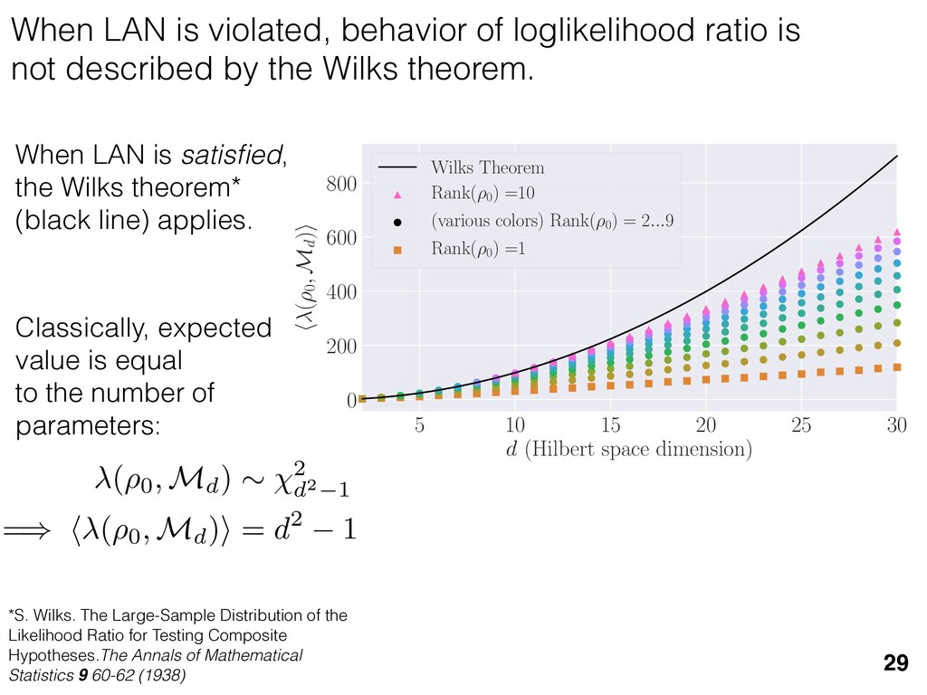
Upgrade to Pro — share decks privately, control downloads, hide ads and more …

Towards Scalable Characterization of Noisy, Intermediate-Scale Quantum Information Processors

Travis Scholten
September 26, 2018
18

Towards Scalable Characterization of Noisy, Intermediate-Scale Quantum Information Processors

My thesis defense talk at the Center for Quantum Information and Control at the University of New Mexico.

Travis Scholten

September 26, 2018
Tweet

More Decks by Travis Scholten

Transcript

  1. Towards Scalable Characterization of Noisy, Intermediate-Scale Quantum Information Processors Travis

    L Scholten @Travis_Sch Center for Quantum Information and Control, UNM 2018 September 26
  2. Quantum computing is entering the Noisy, Intermediate- Scale Quantum (NISQ)

    era*. *J. Preskill, arXiv: 1801.00862 Quantum information processors (QIPs) growing: 1 or 2 qubits to 10-50+. IBM “Yorktown”: 5 IBM “Rueschlikon”: 16 Rigetti “Acorn”: 19 UMD ion chain Rigetti “Agave”: 8 NIST ion trap Figure 1: (a) Scanning electron microscope image of a device similar to the one measured showing the poly-Si gate structure. The blue overlay represents the regions where electrons accumulate below the Si-SiO2 interface. The device is entirely based on CMOS technology and can thus be readily fabricated with existing foundry tools. (b) Schematic cross-section of the device stack (not to scale). The gate oxide is 35 nm thick, the poly-Si gates 200 nm. The active silicon region is enriched 28Si with 500 ppm residual 29Si. (c) The SET charge sensor Figure 3: (a) Charge stability diagram showing the derivative of the CS SNL silicon quantum dot 37
  3. To understand a QIP’s behavior, we use quantum characterization, validation,

    and verification (QCVV). e.g., density matrices, process matrices, gate sets, Hamiltonians/Lindbladians Experimental data D D Property of interest P P Estimated parameters ˆ ✓ ˆ ✓ QCVV model M(✓) M(✓) Goal of QCVV Traditional QCVV methodology: 36
  4. As the NISQ era gets underway, new QCVV techniques will

    be required. More qubits: more resources* required More qubits: new kinds of noise More qubits: holistic characterization necessary No crosstalk Crosstalk/long range correlations possible *time, effort, experiments 6= 35 ⇢ = ✓ · · · · ◆ ⇢ = 0 B B @ · · · · · · · · · · · · · · · · 1 C C A ⇢ = 0 B B B B B B B B B B B B @ · · · · · · · · · · · · · · · · · · · · · · · · · · · · · · · · · · · · · · · · · · · · · · · · · · · · · · · · · · · · · · · · · · · · · · · · · · · · · · · · · 1 C C C C C C C C C C C C A
  5. My research develops ideas for how scalable QCVV techniques could

    be created for NISQ processors. Within traditional QCVV methodology Outside traditional QCVV methodology 34 Experimental data D D Property of interest P P Estimated parameters ˆ ✓ ˆ ✓ QCVV model M(✓) M(✓) Goal of QCVV QCVV models have boundaries, posing problems for model selection. Developing new QCVV techniques requires time and effort. How do model selection techniques behave when boundaries are present? Can machine learning algorithms learn new QCVV techniques? Experimental data D D Property of interest P P Estimated parameters ˆ ✓ ˆ ✓ QCVV model M(✓) M(✓) Goal of QCVV “Machine-learned” QCVV
  6. Chapter 3 Impact of state-space geometry on tomography There are

    three kinds of lies: lies, damned lies, and statistics. - Mark Twain, 1906 To characterize NISQ devices, simpler models that describe their behavior are re- quired. This chapter introduces the idea of statistical model selection, and shows how commonly-used model selection techniques in classical statistical inference problems cannot be blithely applied to models describing a quantum information processor. To (collaboration with Robin Blume-Kohout; published as 2018 New J. Phys. 20 023050) 33
  7. QCVV models have constraints. This causes problems when doing statistical

    model selection. Model selection: choose between 2+ models Prototyping problem: choose a Hilbert space dimension (state tomography) |0i |1i |1i |0i |2i Constrained models violate LAN. M satisfies LAN =) ˆ ⇢ML,M ⇠ N(⇢0, F 1) ⇢ 0 ⇢ 0 ⇢ 0 ⇢ 0 ˆ ⇢ML,M 6⇠ N ( ⇢0, F 1 ) Md = {⇢ 2 B(Hd) | Tr(⇢) = 1, ⇢ 0} *Le Cam L., Yang G.L. (2000) Local Asymptotic Normality. In: Asymptotics in Statistics. Unconstrained models satisfy local asymptotic normality (LAN)*. ⇢ = ✓ a b b? c ◆ ⇢ = 0 @ a b d b? c e d? e? f 1 A ( Md, Md0 ) = 2 log ✓ L ( Md) L ( Md0 ) ◆ Model: Compare using loglikelihood ratio: Required for most model selection techniques! 32 M2 M3
  8. To get a handle on how convex boundaries violate LAN

    we introduced a new generalization of LAN, MP-LAN. satisfies LAN satisfies “MP-LAN” M0 M Quantum state space satisfies MP-LAN! (lift positivity constraint) (all density matrices) (Likelihood is twice continuously differentiable, so it satisfies LAN.) MH = {⇢ | ⇢ 2 B(H), Tr(⇢) = 1, ⇢ 0} and take M0 H = { | 2 B(H), Tr( ) = 1} The main definitions and results required for the remainder of the paper are presented in this subsection. Technical details and proofs are presented in the next subsection. Definition 1 (Metric-projected local asymptotic normality, or MP-LAN). A model M satisfies MP-LAN if M is a convex subset of a model M0 that satisfies LAN. The model M0 will be used to define a set of unconstrained ML estimates ˆ ⇢ ML ,M0 , some of which may not satisfy the positivity constraint. While there are many possible choices for this “unconstrained model” M0, we will find it useful to let M0 be a model whose dimension is the same as M, but where any of the constraints that define M are lifted. (For example, in Lemma 5, we will take M0 to be Hermitian matrices of dimension d.) Other choices of M0 are possible, but we do not explore those here. Although the definition of MP-LAN is rather short, it implies some very useful properties. These properties follow from the fact that, as N ! 1, the behavior of ˆ ⇢ ML ,M and is entirely determined by their behavior in an arbitrarily small region of M around ⇢ 0 , which we call the local state space. 31 Let
  9. We proved models that satisfy MP-LAN have several properties in

    the asymptotic limit. 2. Loglikelihood ratio statistic is equal to Fisher-adjusted squared error 1. is “metric projection” of onto the tangent cone at , . ˆ ⇢ML,M = argmin ⇢2T (⇢0) Tr[(⇢ ˆ ⇢ML,M0 )F(⇢ ˆ ⇢ML,M0 )] ⇢0 ˆ ⇢ML,M T(⇢0 ) M M0 ˆ ⇢ML,M0 Tangent Cone Example (Rebit) (Easy to show for models that satisfy LAN) Local geometry of state space is relevant, not global structure! 30 ⇢0 ( ⇢0, M ) = 2 log ✓ L ( ⇢0) L ( M ) ◆ ! Tr [(ˆ ⇢ML,M ⇢0) F (ˆ ⇢ML,M ⇢0)] M M0 ( ⇢0, M ) = 2 log ✓ L ( ⇢0) L (ˆ ⇢ML,M) ◆ ! LAN Tr[( ⇢0 ˆ ⇢ML,M0 ) F ( ⇢0 ˆ ⇢ML,M0 )] Tr[(ˆ ⇢ML,M ˆ ⇢ML,M0 ) F (ˆ ⇢ML,M ˆ ⇢ML,M0 )] Why nontrivial: Tangent cone factorizes: T(⇢0) = Rd(⇢0) ⌦ C(⇢0) (T(⇢0) = R ⌦ R +) ˆ ⇢ML,M ˆ ⇢ML,M0 T(⇢0)
  10. When LAN is satisfied, the Wilks theorem* (black line) applies.

    Classically, expected value is equal to the number of parameters: *S. Wilks. The Large-Sample Distribution of the Likelihood Ratio for Testing Composite Hypotheses.The Annals of Mathematical Statistics 9 60-62 (1938) When LAN is violated, behavior of loglikelihood ratio is not described by the Wilks theorem. 29 5 10 15 20 25 30 d (Hilbert space dimension) 0 200 400 600 800 h (⇢0 , Md )i Wilks Theorem Rank(⇢0 ) =10 (various colors) Rank(⇢0 ) = 2...9 Rank(⇢0 ) =1 (⇢0, Md) ⇠ 2 d2 1 =) h (⇢0, Md)i = d2 1
  11. 11 2. Deriving an approximation for q proximations of the

    previous section allow us } [ {j } as the ansatz for the eigenvalues of here the pj are N(⇢jj , ✏2) random variables, j are the (fixed, smoothed) order statistics of semicircle distribution. In turn, the defining or q (Equation (12)) is well approximated as r X j =1 (pj q)+ + N X j =1 (j q)+ = 1. this equation, we observe that the j are ally distributed around  = 0, so half of This equation is a quintic polynomial in q/✏, so by the Abel-Ru ni theorem, it has no algebraic solution. How- ever, as N ! 1, its roots have a well-defined algebraic approximation that becomes accurate quite rapidly (e.g., for d r > 4): z ⌘ q/✏ ⇡ 2 p d r ✓ 1 1 2 x + 1 10 x2 1 200 x3 ◆ , (17) where x = ⇣ 15 ⇡r 2( d r ) ⌘ 2 / 5. 3. Expression for h kite i 11 n allow us nvalues of variables, tatistics of e defining mated as This equation is a quintic polynomial in q/✏, so by the Abel-Ru ni theorem, it has no algebraic solution. How- ever, as N ! 1, its roots have a well-defined algebraic approximation that becomes accurate quite rapidly (e.g., for d r > 4): z ⌘ q/✏ ⇡ 2 p d r ✓ 1 1 2 x + 1 10 x2 1 200 x3 ◆ , (17) where x = ⇣ 15 ⇡r 2( d r ) ⌘ 2 / 5. 11 w us s of bles, s of ning as This equation is a quintic polynomial in q/✏, so by the Abel-Ru ni theorem, it has no algebraic solution. How- ever, as N ! 1, its roots have a well-defined algebraic approximation that becomes accurate quite rapidly (e.g., for d r > 4): z ⌘ q/✏ ⇡ 2 p d r ✓ 1 1 2 x + 1 10 x2 1 200 x3 ◆ , (17) where x = ⇣ 15 ⇡r 2( d r ) ⌘ 2 / 5. med N samples is su ciently large , the eigenvalues of ⇢ 0 are large bations jj and q. This implies nder this assumption, q is the (pj q) + N X j =1 (j q)+ = 1 Z 2 ✏ p N  = q ( q)Pr()d = 0 h (q2 + 8N) p q2 + 4N ✓ ⇡ 2 sin 1 ✓ q 2 p N ◆◆ = 0, (15) N(0, r✏2) random variable. We rete sum (line 1) with an inte- ximation is valid when N 1, roximate a discrete collection of ers by a smooth density or dis- umbers that has approximately remarkably accurate in practice. imation, we replace with its zero. We could obtain an even n by treating more carefully, tion turns out to be quite accu- ), it is necessary to further sim- pression resulting from the inte- we assume ⇢ 0 is relatively low- given in Equation (13): h kite i ⇡ 1 ✏2 * r X j =1 [⇢jj (pj q)+]2 + N X j =1 ⇥ (¯ j q)+ ⇤ 2 + ⇡ 1 ✏2 * r X j =1 [ jj + q]2 + N X j =1 ⇥ (¯ j q)+ ⇤ 2 + ⇡ r + rz2 + N ✏2 Z 2 ✏ p N  = q Pr()( q)2d = r + rz2 + N(N + z2) ⇡ ✓ ⇡ 2 sin 1 ✓ z 2 p N ◆◆ z(z2 + 26N) 24⇡ p 4N z2 . (18) D. Complete Expression for h i The total expected value, h i = h L i + h kite i, is thus h (⇢ 0 , Md)i ⇡ 2rd r2 + rz2 + N(N + z2) ⇡ ✓ ⇡ 2 sin 1 ✓ z 2 p N ◆◆ z(z2 + 26N) 24⇡ p 4N z2 . (19) where z is given in Equation (17), N = d r, and r = Rank(⇢ 0 ). When LAN is violated, our result (dashed lines) applies. r X j =1 (pj q) + N X j =1 (j q)+ = 1 =) rq + + N Z 2 ✏ p N  = q ( q)Pr()d = 0 ) rq + + ✏ 12⇡ h (q2 + 8N) p q2 + 4N 12qN ✓ ⇡ 2 sin 1 ✓ q 2 p N ◆◆ = 0, (15) = Pr j =1 jj is a N(0, r✏2) random variable. We to replace a discrete sum (line 1) with an inte- ine 2). This approximation is valid when N 1, can accurately approximate a discrete collection of spaced real numbers by a smooth density or dis- on over the real numbers that has approximately me CDF. It is also remarkably accurate in practice. et another approximation, we replace with its e value, which is zero. We could obtain an even accurate expression by treating more carefully, is crude approximation turns out to be quite accu- ready. olve Equation (15), it is necessary to further sim- he complicated expression resulting from the inte- ine 3). To do so, we assume ⇢ 0 is relatively low- so r ⌧ d/2. In this case, the sum of the positive ⇡ ✏2 j =1 [ jj + q]2 + j =1 (¯ j q ⇡ r + rz2 + N ✏2 Z 2 ✏ p N  = q Pr()( q)2 = r + rz2 + N(N + z2) ⇡ ✓ ⇡ 2 sin 1 z(z2 + 26N) 24⇡ p 4N z2 . D. Complete Expression for h The total expected value, h i = h L i + h h (⇢ 0 , Md)i ⇡ 2rd r2 + rz2 + N(N + z2) ⇡ ✓ ⇡ 2 sin 1 ✓ z(z2 + 26N) 24⇡ p 4N z2 . where z is given in Equation (17), N = d Rank(⇢ 0 ). V. COMPARISON TO NUMER kite i ⇡ 1 ✏2 * r X j =1 [⇢jj (pj q)+]2 + N X j =1 ⇥ (¯ j q)+ ⇤ 2 + ⇡ 1 ✏2 * r X j =1 [ jj + q]2 + N X j =1 ⇥ (¯ j q)+ ⇤ 2 + ⇡ r + rz2 + N ✏2 Z 2 ✏ p N  = q Pr()( q)2d = r + rz2 + N(N + z2) ⇡ ✓ ⇡ 2 sin 1 ✓ z 2 p N ◆◆ z(z2 + 26N) 24⇡ p 4N z2 . (18) D. Complete Expression for h i The total expected value, h i = h L i + h kite i, is thus h (⇢ 0 , Md)i ⇡ 2rd r2 + rz2 + N(N + z2) ⇡ ✓ ⇡ 2 sin 1 ✓ z 2 p N ◆◆ z(z2 + 26N) 24⇡ p 4N z2 . (19) here z is given in Equation (17), N = d r, and r = on, q is the q)+ = 1 )d = 0 4N ◆◆ = 0, (15) variable. We ith an inte- hen N 1, collection of nsity or dis- proximately in practice. with its ain an even re carefully, e quite accu- further sim- ✏2 j =1 j =1 ⇡ 1 ✏2 * r X j =1 [ jj + q]2 + N X j =1 ⇥ (¯ j q)+ ⇤ 2 + ⇡ r + rz2 + N ✏2 Z 2 ✏ p N  = q Pr()( q)2d = r + rz2 + N(N + z2) ⇡ ✓ ⇡ 2 sin 1 ✓ z 2 p N ◆◆ z(z2 + 26N) 24⇡ p 4N z2 . (18) D. Complete Expression for h i The total expected value, h i = h L i + h kite i, is thus h (⇢ 0 , Md)i ⇡ 2rd r2 + rz2 + N(N + z2) ⇡ ✓ ⇡ 2 sin 1 ✓ z 2 p N ◆◆ z(z2 + 26N) 24⇡ p 4N z2 . (19) where z is given in Equation (17), N = d r, and r = Rank(⇢ 0 ). Constrained models have an “effective” number of parameters We used MP-LAN to compute an accurate formula for the expected value of the loglikelihood ratio statistic. (Details: 2018 New J. Phys. 20 023050) 28 5 10 15 20 25 30 d (Hilbert space dimension) 0 200 400 600 800 h (⇢0 , Md )i Wilks Theorem Rank(⇢0 ) =10 (various colors) Rank(⇢0 ) = 2...9 Rank(⇢0 ) =1
  12. Recap: the impact of state-space geometry on tomography Models with

    boundaries do not satisfy LAN. They can satisfy MP-LAN. ⇢ 0 ⇢ 0 ˆ ⇢ML,M 6⇠ N ( ⇢0, F 1 ) = ) M We developed an (approximate) replacement for the Wilks theorem that’s applicable for state tomography. 5 10 15 20 25 30 d (Hilbert Space Dimension) 0 200 400 600 800 h (⇢0 , Md )i An Accurate Replacement for the Wilks Theorem Wilks Theorem Rank(⇢0 ) =10 (various colors) Rank(⇢0 ) = 2...9 Rank(⇢0 ) =1 Application to NISQ: Model selection will be necessary to describe behavior of NISQ processors. These models will have boundaries! They will affect behavior of model selection techniques. Use them wisely and carefully! 27
  13. Chapter 4 Other applications of MP-LAN I suppose it is

    tempting, if the only tool you have is a hammer, to treat everything as if it were a nail. - Abraham Maslow, 1966 [211] The generalization of LAN given in Chapter 3 (MP-LAN) was extremely useful for understanding the behavior of the maximum likelihood (ML)1 estimator in state tomography. This chapter explores other applications of MP-LAN. The first connects MP-LAN to quantum compressed sensing, where I show that the expected rank of ML (independent work; unpublished) 26
  14. 1. ML state tomography is self-certifying: all non-zero eigenvalues of

    the true state will be inferred. Using MP-LAN, I examined other asymptotic properties of the maximum likelihood (ML) estimator. 2. MP-LAN formalism lets us compute in some cases. .17 0 0 .5 .5 0 .33 .5 1 (classical 3-simplex; estimating a “noisy die”*) - Rank of estimates at least as high as rank of truth. - But not much higher. Rank(⇢0) 1 2 3 Pr(Rank(ˆ ⇢ML) = 1) Pr (Rank(ˆ ⇢ML) = 2) Pr (Rank(ˆ ⇢ML) = 3) *Ferrie and Blume-Kohout, AIP Conference Proceedings 1443, 14 (2012) 25 Pr(Rank(ˆ ⇢ML))
  15. 5 10 15 20 25 30 35 40 d (Hilbert

    space dimension) 5 10 15 20 hRank(ˆ ⇢ML,d )i Expected rank of ML estimates Rank(⇢0 ) =1 (various colors) Rank(⇢0 ) = 2...9 Rank(⇢0 ) =10 3. ML state tomography gives low-rank estimates “for free” when the true state is low rank. Using MP-LAN, I examined other asymptotic properties of the maximum likelihood (ML) estimator. Slow growth! 24 d = 20, Rank(⇢0) = 1 Quantum state-space geometry leads to concentration of . Pr(Rank(ˆ ⇢ML))
  16. Chapter 5 Machine-learned QCVV techniques Machines take me by surprise

    with great frequency. - Alan Turing (1950) [306] Designing a QCVV technique to probe a new property of interest takes time, ef- fort, and expertise. Machine learning (ML1 ) can help automate the development of new QCVV techniques. In this chapter, I investigate the geometry of QCVV data (collaboration with Yi-Kai Liu (UMD/NIST), Kevin Young (SNL), Robin Blume-Kohout; in preparation for arXiv) 22
  17. Experimental data D D Property of interest P P Estimated

    parameters ˆ ✓ ˆ ✓ QCVV model M(✓) M(✓) Goal of QCVV Why investigating “machine-learned” QCVV techniques could be worthwhile. QCVV technique ML algorithm Extensive domain- specific expertise Characterize QIP property Cognitive effort/time TASK RESOURCES TOOL Leverage QCVV know-how in a new way Eliminate statistical models to describe a QIP’s behavior Natural way to frame QCVV tasks as ML problems “Infer type of noise” = classification “Infer strength of noise” = regression 21
  18. A “machine-learned” QCVV technique has a few more components than

    traditional QCVV techniques. Represent data in a way that can be processed by algorithms What a machine-learned QCVV technique looks like Example instances to train on Chosen based on task Evaluate performance of analysis function Experimental data D D Property of interest P P Goal of QCVV Feature map Data collection C C ML algorithm A A Performance measure P P Analysis function f f No model… & no parameter estimation! 20
  19. We prototyped machine-learned QCVV by using ML algorithms to classify

    noise acting on a single qubit QIP. using standard time consuming ackage designed quantum circuit rray. In a mat- yntax and start rcuit from the they’ve learned nd of § IV, but at wish to type- NU public license. C. \ ket { A } | A i \ bra { B } h B | \ ip { A }{ B } h A | B i \ op { A }{ B } | A ih B | \ melem { j }{ B }{ k } h j | B | k i \ expval { B } h B i IV. SIMPLE QUANTUM CIRCUITS To begin, suppose the reader would like to typeset the following simple circuit: X ⇢ GX GY GY GI M This was typeset using “GxGyGyGi”: Black-box, single-qubit QIP described by a gate set Experiments on the QIP are specified as circuits: ⇢ M GX GI GY Push buttons… …do operations Our prototyping problem: distinguishing coherent and stochastic noise. 19 Action on Bloch sphere G = {⇢, M, GI, GX, GY }
  20. Noisy unitary channels described by error generator: Error generator derived

    from solution to the time-homogeneous Lindblad equation: Our prototyping problem: coherent vs stochastic noise Coherent: only Hamiltonian errors Stochastic: fluctuations that average to the desired Hamiltonian We prototyped machine-learned QCVV by using ML algorithms to classify noise acting on a single qubit QIP. 18 H = H0 + He , h = 0 H = H0 , h 0, h 6= 0 G0[ ⇢ ] = U⇢U†, where U = e iH0 = eH0 [ ⇢ ] , where H0[ ⇢ ] = i [ H0 , ⇢ ] Under noise: G0 ! G = eL [ ⇢ ] ˙ ⇢ = L[⇢] where L[⇢] = i ~ [H, ⇢] + d2 1 X j,k=1 hjk  Aj ⇢A† k 1 2 {A† k Aj , ⇢} =) ⇢(t) = eLt[⇢(0)]
  21. The other components need to be specified as well! We

    used… Experimental data D D Property of interest P P Goal of QCVV Feature map Data collection C C ML algorithm A A Performance measure P P Analysis function f f Experimental data Gate set tomography (GST) experiment design Feature map Treat outcome probabilities as a feature vector ## Columns = minus count, plus count {} 100 0 Gx 44 56 Gy 45 55 GxGx 9 91 GxGxGx 68 32 GyGyGy 70 30 f = (f1, f2, · · · ) 2 Rd Data collection Numerically-simulated GST data sets ML algorithm Supervised binary classifiers Performance measure Classification accuracy 17
  22. To do machine learning on GST data sets, we embed

    them in a feature space. Feature space dimension grows with L b/c more circuits are added to the experiment design. 0 50 100 150 200 250 Maximum circuit depth L 0 500 1000 1500 2000 2500 Feature space dimension d GST experiment designs form a family, parameterized by an index L. Circuit depth is bounded: L + O(1). # of circuits design depends on L. {} Gx Gy GxGx GxGxGx GyGyGy GxGy GxGxGxGx GxGyGyGy GyGx GyGy GyGxGx GyGxGxGx GyGyGyGy GxGxGy GxGxGxGxGx GxGxGyGyGy GxGxGxGy GxGxGxGxGxGx GxGxGxGyGyGy GyGyGyGx GyGyGyGxGx GyGyGyGxGxGx GyGyGyGyGyGy (Gi) (Gi)Gx (Gi)Gy (Gi)GxGx (Gi)GxGxGx (Gi)GyGyGy Gx(Gi) Gx(Gi)Gx Gx(Gi)Gy Gx(Gi)GxGx Gx(Gi)GxGxGx Gx(Gi)GyGyGy Gy(Gi) Gy(Gi)Gx Gy(Gi)Gy Gy(Gi)GxGx Gy(Gi)GxGxGx Gy(Gi)GyGyGy GxGx(Gi) GxGx(Gi)Gx GxGx(Gi)Gy GxGx(Gi)GxGx GxGx(Gi)GxGxGx GxGx(Gi)GyGyGy GxGxGx(Gi) GxGxGx(Gi)Gx GxGxGx(Gi)Gy GxGxGx(Gi)GxGx GxGxGx(Gi)GxGxGx GxGxGx(Gi)GyGyGy GyGyGy(Gi) GyGyGy(Gi)Gx GyGyGy(Gi)Gy GyGyGy(Gi)GxGx GyGyGy(Gi)GxGxGx GyGyGy(Gi)GyGyGy Gy(Gx)Gy Gy(Gx)GxGxGx Gy(Gx)GyGyGy GxGxGx(Gx)Gy GxGxGx(Gx)GxGxGx GxGxGx(Gx)GyGyGy GyGyGy(Gx)Gy GyGyGy(Gx)GxGxGx GyGyGy(Gx)GyGyGy Gx(Gy)Gx Gx(Gy)Gy Gx(Gy)GxGx Gx(Gy)GxGxGx Gx(Gy)GyGyGy Gy(Gy)Gx Gy(Gy)GxGx Gy(Gy)GxGxGx Gy(Gy)GyGyGy GxGx(Gy)Gx GxGx(Gy)Gy GxGx(Gy)GxGx GxGx(Gy)GxGxGx GxGx(Gy)GyGyGy GxGxGx(Gy)Gx GxGxGx(Gy)Gy GxGxGx(Gy)GxGx GxGxGx(Gy)GxGxGx GxGxGx(Gy)GyGyGy GyGyGy(Gy)Gx GyGyGy(Gy)GxGx GyGyGy(Gy)GxGxGx GyGyGy(Gy)GyGyGy L=1 GST experiment design # of circuits design = dimension of feature space. L = 1 : f = (f1, · · · , f92) 16
  23. We investigated 5 simple ML algorithms for supervised binary classification

    Linear (hyperplane) Nonlinear (hypersurface) Linear algorithms Linear discriminant analysis (statistically) optimal hyperplane for Gaussian data w/ same covariance Linear support vector machine highest margin hyperplane Perceptron simple-to-use algorithm; guaranteed to find a hyperplane if it exists Nonlinear algorithms Quadratic discriminant analysis (statistically) optimal hypersurface for Gaussian data w/ different covariance Radial basis function support vector machine implicit mapping to high-dimensional feature space, and then find highest- margin hyperplane 15
  24. Out-of-the-box performance varies depending on ML algorithm and GST experiment

    design. Longer circuits = amplify noise more = higher accuracy Shorter circuits = low accuracy?? Why do the algorithms perform poorly? 14
  25. Hyperparameter tuning is an easy, automatable way to influence the

    accuracy of the analysis map. Hyperparameters = parameters that control algorithm’s behavior Tuning usually boosts accuracy…yet linear algorithms on L=1 GST data do poorly. Why? L=1 GST is “complete”, but geometry of the data is not suitable for linear classifiers. 13
  26. The geometry of L=1 GST data is not amenable for

    learning by linear classification algorithms. Dimensionality reduction shows L=1 data looks like a radio dish. Corroborated by intuition from Choi-Jamiolkowski isometry: Coherent noise -> pure states Stochastic noise -> mixed states No hyperplane can separate the data! Use new feature maps to “unroll” radio dish SQ : D ! (f1, f2, · · · , fd, f2 1 , f2 2 , · · · , f2 d ) PP : D ! (f1, · · · fd, f2 1 , f1f2, · · · , fd 1fd, f2 d ) 12
  27. Feature engineering changes geometry of L=1 data, and boosts performance

    of (some) linear classifiers. 0.75 0.80 0.85 0.90 0.95 1.00 QDA RBF SVM 0.75 0.80 0.85 0.90 0.95 1.00 Accuracy LDA Linear SVM Perceptron QDA RBF SVM Algorithm Tuned hyperparameters Feature map SQ PP L=1 most naturally separated by a quartic surface, but it is well-approximated by a quadratic one. Algorithm makes bad assumptions about data (Gaussian w/ same covariance), so it performs poorly. 11
  28. Hyperparameter tuning and feature engineering enables (some) linear classifiers to

    achieve high accuracy. 10 0.75 0.80 0.85 0.90 0.95 1.00 LDA Linear SVM Perceptron QDA RBF SVM Algorithm Default hyperparameters 0.75 0.80 0.85 0.90 0.95 1.00 Accuracy LDA Linear SVM Perceptron QDA RBF SVM Algorithm Tuned hyperparameters Feature map SQ PP LDA Linear SVM Perceptron QDA RBF SVM from sklearn import * L=1
  29. Recap: machine-learned QCVV techniques Machine-learned QCVV is possible. Leveraging ML

    algorithms requires framing the QCVV task in the language of ML. Experimental data D D Property of interest P P Goal of QCVV Feature map Data collection C C ML algorithm A A Performance measure P P Analysis function f f Many QCVV tasks can be framed as supervised learning problems. For the prototyping problem, feature engineering + hyperparameter tuning lets (some) linear algorithms succeed. 0.75 0.80 0.85 0.90 0.95 1.00 LDA Linear SVM Perceptron QDA RBF SVM Algorithm Default hyperparameters 0.75 0.80 0.85 0.90 0.95 1.00 Accuracy LDA Linear SVM Perceptron QDA RBF SVM Algorithm Tuned hyperparameters Feature map SQ PP Application to NISQ: properties we care about may be hard to extract from data using statistical models. Deploy ML algorithms instead. 9
  30. (recent, independent work; unpublished) Chapter 6 Machine-learned experiment design for

    QCVV The design of experiments is, however, too large a subject, and of too great importance to the general body of scientific workers, for any incidental treatment to be adequate. - Ronald A. Fisher, 1935 [106] Chapter 5 focused on how ML1 algorithms can help with data processing, by learning inference tools for a targeted characterization problem on a qubit. This chapter investigates how ML can improve the other component of QCVV techniques, the experiment design. I show that ML algorithms for “feature selection” can pare 8
  31. ML algorithms are good for data processing… what about designing

    QCVV experiments? Experiment design = set of circuits a QIP runs for QCVV Simple way to generate new experiment designs: take a large (many-circuit) design and prune it. Leverage QCVV knowledge to develop large design, and ML capabilities to prune it. Prototyping problem: pruning gate set tomography (GST) experiment designs 7 {} Gx Gy GxGx GxGxGx GyGyGy GxGy GxGxGxGx GxGyGyGy GyGx GyGy GyGxGx GyGxGxGx GyGyGyGy GxGxGy GxGxGxGxGx GxGxGyGyGy GxGxGxGy GxGxGxGxGxGx GxGxGxGyGyGy GyGyGyGx GyGyGyGxGx GyGyGyGxGxGx GyGyGyGyGyGy (Gi) (Gi)Gx (Gi)Gy (Gi)GxGx (Gi)GxGxGx (Gi)GyGyGy Gx(Gi) Gx(Gi)Gx Gx(Gi)Gy Gx(Gi)GxGx Gx(Gi)GxGxGx Gx(Gi)GyGyGy Gy(Gi) Gy(Gi)Gx Gy(Gi)Gy Gy(Gi)GxGx Gy(Gi)GxGxGx Gy(Gi)GyGyGy GxGx(Gi) GxGx(Gi)Gx GxGx(Gi)Gy GxGx(Gi)GxGx GxGx(Gi)GxGxGx GxGx(Gi)GyGyGy GxGxGx(Gi) GxGxGx(Gi)Gx GxGxGx(Gi)Gy GxGxGx(Gi)GxGx GxGxGx(Gi)GxGxGx GxGxGx(Gi)GyGyGy GyGyGy(Gi) GyGyGy(Gi)Gx GyGyGy(Gi)Gy GyGyGy(Gi)GxGx GyGyGy(Gi)GxGxGx GyGyGy(Gi)GyGyGy Gy(Gx)Gy Gy(Gx)GxGxGx Gy(Gx)GyGyGy GxGxGx(Gx)Gy GxGxGx(Gx)GxGxGx GxGxGx(Gx)GyGyGy GyGyGy(Gx)Gy GyGyGy(Gx)GxGxGx GyGyGy(Gx)GyGyGy Gx(Gy)Gx Gx(Gy)Gy Gx(Gy)GxGx Gx(Gy)GxGxGx Gx(Gy)GyGyGy Gy(Gy)Gx Gy(Gy)GxGx Gy(Gy)GxGxGx Gy(Gy)GyGyGy GxGx(Gy)Gx GxGx(Gy)Gy GxGx(Gy)GxGx GxGx(Gy)GxGxGx GxGx(Gy)GyGyGy GxGxGx(Gy)Gx GxGxGx(Gy)Gy GxGxGx(Gy)GxGx GxGxGx(Gy)GxGxGx GxGxGx(Gy)GyGyGy GyGyGy(Gy)Gx GyGyGy(Gy)GxGx GyGyGy(Gy)GxGxGx GyGyGy(Gy)GyGyGy L=1 GST experiment design
  32. {} Gx Gy GxGx GxGxGx GyGyGy GxGy GxGxGxGx GxGyGyGy GyGx

    GyGy GyGxGx GyGxGxGx GyGyGyGy GxGxGy GxGxGxGxGx GxGxGyGyGy GxGxGxGy GxGxGxGxGxGx GxGxGxGyGyGy GyGyGyGx GyGyGyGxGx GyGyGyGxGxGx GyGyGyGyGyGy (Gi) (Gi)Gx (Gi)Gy (Gi)GxGx (Gi)GxGxGx (Gi)GyGyGy Gx(Gi) Gx(Gi)Gx Gx(Gi)Gy Gx(Gi)GxGx Gx(Gi)GxGxGx Gx(Gi)GyGyGy Gy(Gi) Gy(Gi)Gx Gy(Gi)Gy Gy(Gi)GxGx Gy(Gi)GxGxGx Gy(Gi)GyGyGy GxGx(Gi) GxGx(Gi)Gx GxGx(Gi)Gy GxGx(Gi)GxGx GxGx(Gi)GxGxGx GxGx(Gi)GyGyGy GxGxGx(Gi) GxGxGx(Gi)Gx GxGxGx(Gi)Gy GxGxGx(Gi)GxGx GxGxGx(Gi)GxGxGx GxGxGx(Gi)GyGyGy GyGyGy(Gi) GyGyGy(Gi)Gx GyGyGy(Gi)Gy GyGyGy(Gi)GxGx GyGyGy(Gi)GxGxGx GyGyGy(Gi)GyGyGy Gy(Gx)Gy Gy(Gx)GxGxGx Gy(Gx)GyGyGy GxGxGx(Gx)Gy GxGxGx(Gx)GxGxGx GxGxGx(Gx)GyGyGy GyGyGy(Gx)Gy GyGyGy(Gx)GxGxGx GyGyGy(Gx)GyGyGy Gx(Gy)Gx Gx(Gy)Gy Gx(Gy)GxGx Gx(Gy)GxGxGx Gx(Gy)GyGyGy Gy(Gy)Gx Gy(Gy)GxGx Gy(Gy)GxGxGx Gy(Gy)GyGyGy GxGx(Gy)Gx GxGx(Gy)Gy GxGx(Gy)GxGx GxGx(Gy)GxGxGx GxGx(Gy)GyGyGy GxGxGx(Gy)Gx GxGxGx(Gy)Gy GxGxGx(Gy)GxGx GxGxGx(Gy)GxGxGx GxGxGx(Gy)GyGyGy GyGyGy(Gy)Gx GyGyGy(Gy)GxGx GyGyGy(Gy)GxGxGx GyGyGy(Gy)GyGyGy L=1 GST experiment design ML algorithms can be used to select a subset of an original experiment design that is useful for a QCVV task. Task 1 Task 2 Task 3 A proposed design is useful if: a) it has fewer circuits than the original GST design. b) when projected onto the reduced feature space, the data is linearly separable. Components of machine- learned experiment design: - QCVV task - GST experiment design - ML algorithm Simple way to generate new experiment designs: take a large (many-circuit) design and prune it. “feature selection” 6
  33. To demonstrate the viability of machine-learned experiment design, I considered

    4 single-qubit QCVV tasks. Each task of the form “distinguish noise type X from Y”: IV: Pauli vs. non-Pauli stochastic I: Pure-state amplitude damping vs. arbitrary stochastic II: Coherent vs. arbitrary stochastic III: Depolarizing vs. anisotropic Pauli stochastic (Lindblad h-matrix is diagonal) (Lindblad h-matrix is diagonal or weakly, off-diagonally dominant) We require the two noise models to be gapped
 (i.e., distinguishable). 5
  34. IV: Pauli vs. non-Pauli stochastic I: Pure-state amplitude damping vs.

    arbitrary stochastic II: Coherent vs. arbitrary stochastic III: Depolarizing vs. anisotropic Pauli stochastic 5 The number of circuits can be reduced by >85% for every property I considered. r = #circuits selected #circuits in original design r = .023 r = .039 r = .048 r = .132 (Relates to gap?)
  35. ML algorithms for feature selection fall into three categories. I

    investigated algorithms in two of them. Filter: preprocess based on measure of importance Do PCA & keep features used in dimensionality reduction Run a perceptron & keep features based on sensitivity for classification Estimate mutual information (MI) 0 1 X 0.0 0.5 1.0 Y Zero MI 0 1 X 0.0 0.5 1.0 Y Moderate MI 0 1 X 0.0 0.5 1.0 Y High MI 0 1 2 3 4 5 6 7 8 9 10 11 12 13 14 15 16 17 18 19 Number of PCA components q 0.4 0.6 0.8 1.0 Cumulative explained variance ratio Determining a su cient number of PCA components 2 1 0 1 2 4 2 0 2 [0.01 ⇤ x + 2.8 ⇤ y + 0.0 = 0] 3 2 1 0 1 2 4 2 0 2 4 [ 1.64 ⇤ x + 2.28 ⇤ y + 0.0] Wrapper: combine feature selection with solving the ML task L1-regularized support vector machine* 3 *not maximal-margin!
  36. Next step: understand why different algorithms, experiment designs, and feature

    maps lead to different reductions. 2 r I II III IV .023 .039 .048 .132 Best performance: Higher-L experiment design & using feature engineering seems to help. Again, maximal amount of reduction yet unknown. IV: Pauli vs. non-Pauli stochastic I: Pure-state amplitude damping vs. arbitrary stochastic II: Coherent vs. arbitrary stochastic III: Depolarizing vs. anisotropic Pauli stochastic
  37. Recap: machine-learned experiment design for QCVV {} Gx Gy GxGx

    GxGxGx GyGyGy GxGy GxGxGxGx GxGyGyGy GyGx GyGy GyGxGx GyGxGxGx GyGyGyGy GxGxGy GxGxGxGxGx GxGxGyGyGy GxGxGxGy GxGxGxGxGxGx GxGxGxGyGyGy GyGyGyGx GyGyGyGxGx GyGyGyGxGxGx GyGyGyGyGyGy (Gi) (Gi)Gx (Gi)Gy (Gi)GxGx (Gi)GxGxGx (Gi)GyGyGy Gx(Gi) Gx(Gi)Gx Gx(Gi)Gy Gx(Gi)GxGx Gx(Gi)GxGxGx Gx(Gi)GyGyGy Gy(Gi) Gy(Gi)Gx Gy(Gi)Gy Gy(Gi)GxGx Gy(Gi)GxGxGx Gy(Gi)GyGyGy GxGx(Gi) GxGx(Gi)Gx GxGx(Gi)Gy GxGx(Gi)GxGx GxGx(Gi)GxGxGx GxGx(Gi)GyGyGy GxGxGx(Gi) GxGxGx(Gi)Gx GxGxGx(Gi)Gy GxGxGx(Gi)GxGx GxGxGx(Gi)GxGxGx GxGxGx(Gi)GyGyGy GyGyGy(Gi) GyGyGy(Gi)Gx GyGyGy(Gi)Gy GyGyGy(Gi)GxGx GyGyGy(Gi)GxGxGx GyGyGy(Gi)GyGyGy Gy(Gx)Gy Gy(Gx)GxGxGx Gy(Gx)GyGyGy GxGxGx(Gx)Gy GxGxGx(Gx)GxGxGx GxGxGx(Gx)GyGyGy GyGyGy(Gx)Gy GyGyGy(Gx)GxGxGx GyGyGy(Gx)GyGyGy Gx(Gy)Gx Gx(Gy)Gy Gx(Gy)GxGx Gx(Gy)GxGxGx Gx(Gy)GyGyGy Gy(Gy)Gx Gy(Gy)GxGx Gy(Gy)GxGxGx Gy(Gy)GyGyGy GxGx(Gy)Gx GxGx(Gy)Gy GxGx(Gy)GxGx GxGx(Gy)GxGxGx GxGx(Gy)GyGyGy GxGxGx(Gy)Gx GxGxGx(Gy)Gy GxGxGx(Gy)GxGx GxGxGx(Gy)GxGxGx GxGxGx(Gy)GyGyGy GyGyGy(Gy)Gx GyGyGy(Gy)GxGx GyGyGy(Gy)GxGxGx GyGyGy(Gy)GyGyGy Task 1 Task 2 Task 3 L=1 GST experiment design Circuit reduction using feature selection algorithms is possible. Need to understand why different algorithms perform the way they do. What other properties should we demand of reduced feature space? 1