Machine Learning with TensorFlow

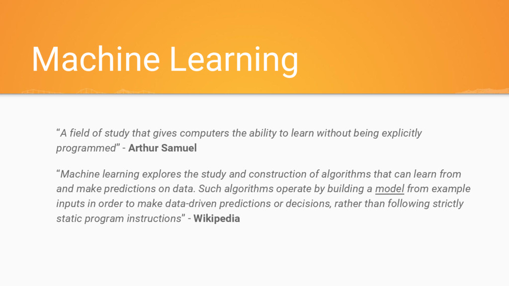
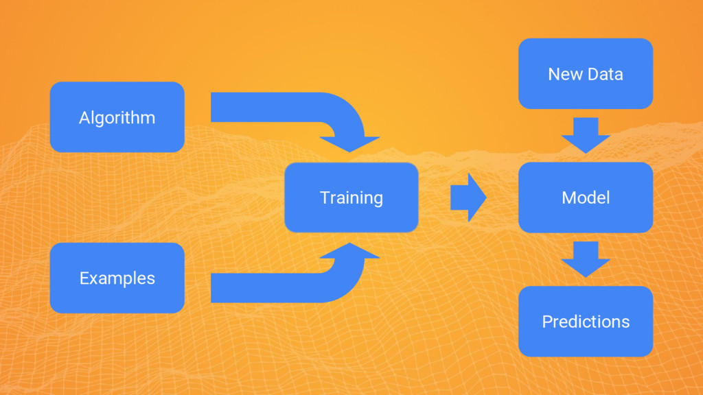
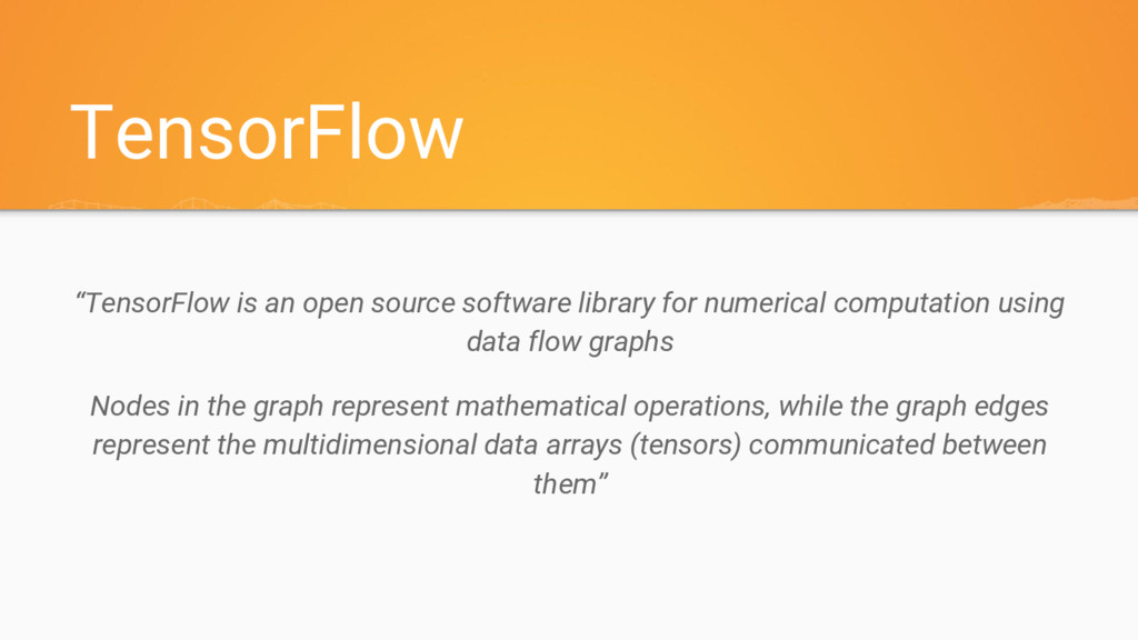
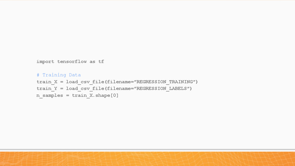
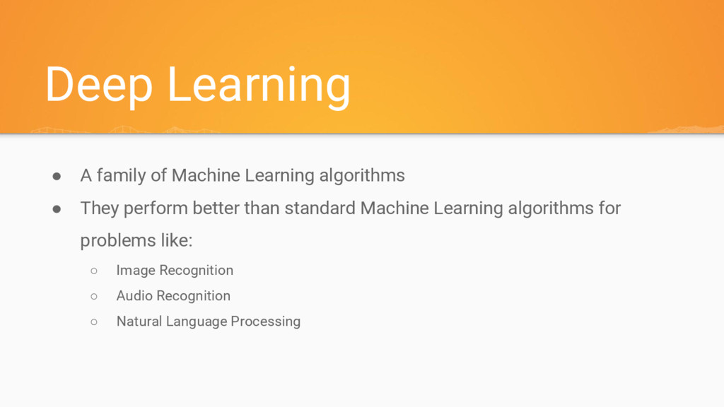
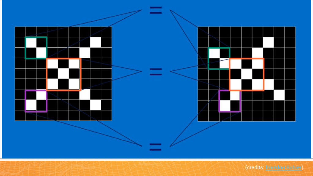
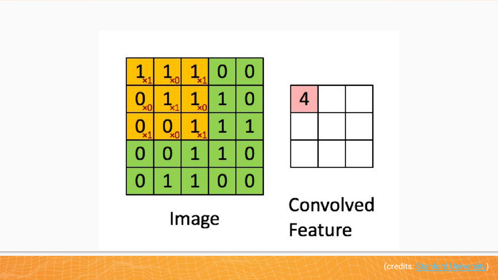
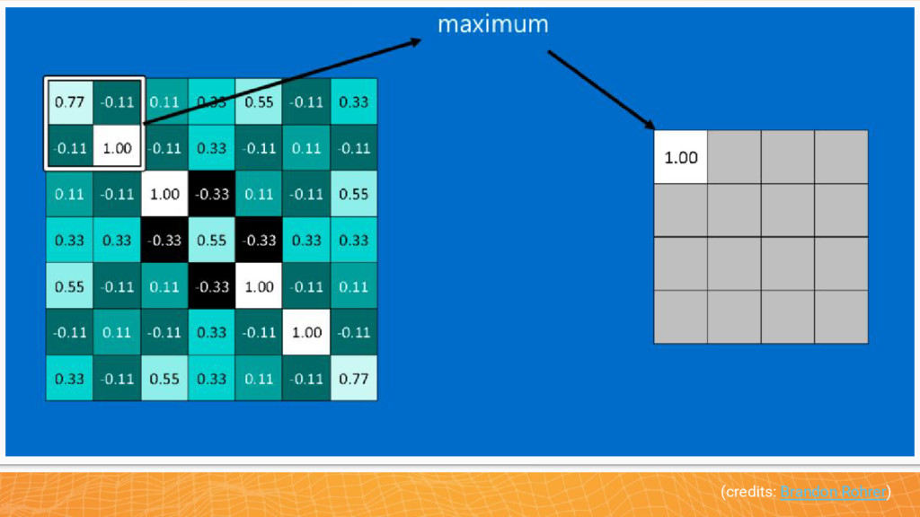
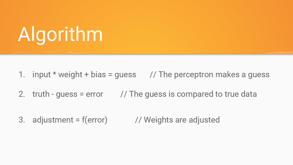
TensorFlow is an open source software library for machine learning in various kinds of tasks, from natural language processing to image recognition. TensorFlow was originally developed by the Google Brain team for Google's research purposes and later released as Open Source software under the Apache 2.0 license.
In this talk we will use a "hands-on" approach to explore its potential and see how the construction of predictive models becomes simpler.

Transcript

1. Machine Learning with TensorFlow GDG Milano TAG Milano 17 October 2016 #Google #TensorFlow #ML
2. Preamble
3. You must be this unprepared to ride Machine Learning: Low Machine Learning: High TensorFlow: Low TensorFlow: High
4. Machine? Learning?
5. Machine Learning “A field of study that gives computers the ability to learn without being explicitly programmed” - Arthur Samuel “Machine learning explores the study and construction of algorithms that can learn from and make predictions on data. Such algorithms operate by building a model from example inputs in order to make data-driven predictions or decisions, rather than following strictly static program instructions” - Wikipedia
6. Predictive Model “Representation of a phenomenon. “It can be used to generate knowledge from data and to predict an outcome.”
7. Algorithm Examples Training Model New Data Predictions
8. Linear Regression
9. Predicting House Prices • Suppose you want to sell your house, but you don't know how much to list it for • How to estimate the value of the house? • It might make sense to look at other recent sales in your neighborhood
10. Feature Selection • What makes two houses “similar”? • We are going to assume that, with respect to real estate sales, what makes two houses similar is their size
11. Square Feet Price ( $ ) f(x) = w0 x + w1
12. Who is right? We need a way to find out how good bad is the model
13. Square Feet Price ( $ )
14. How can we solve this?
15. (credits: Sebastian Raschka)
16. 1. input * weight + bias = guess // The algorithm makes a guess 2. truth - guess = error // The guess is compared to true data 3. adjustment = f(error) // Weights are adjusted Algorithm
18. TensorFlow “TensorFlow is an open source software library for numerical computation using data flow graphs Nodes in the graph represent mathematical operations, while the graph edges represent the multidimensional data arrays (tensors) communicated between them”
19. Data Flow Graph Computation is defined as a directed acyclic graph (DAG) to optimize an objective function • Graph is defined in high-level language • Graph is compiled and optimized • Graph is executed on available low level devices (CPU, GPU) • Data flow through the graph
20. Tensorflow Operations Operation Description tf.add sum tf.sub substraction tf.mul multiplication tf.div division tf.mod module tf.abs absolute value tf.neg negative value tf.inv inverse tf.maximum returns the maximum tf.minimum returns the minimum Operation Description tf.square calculates the square tf.round nearest integer tf.sqrt square root tf.pow calculates the power tf.exp exponential tf.log logarithm tf.cos calculates the cosine tf.sin calculates the sine tf.matmul tensor product tf.transpose tensor transpose
22. “Hello World” Example
23. import tensorflow as tf # Create a Constant op that produces a 1x2 matrix. The op is # added as a node to the default graph. # # The value returned by the constructor represents the output # of the Constant op. matrix1 = tf.constant([[3., 3.]]) # Create another Constant that produces a 2x1 matrix. matrix2 = tf.constant([[2.],[2.]]) # Create a Matmul op that takes 'matrix1' and 'matrix2' as inputs. # The returned value, 'product', represents the result of the matrix # multiplication. product = tf.matmul(matrix1, matrix2)
24. Holy Moly! It’s not working!
25. # Launch the default graph. sess = tf.Session() # To run the matmul op we call the session 'run()' method, passing 'product' # which represents the output of the matmul op. This indicates to the call # that we want to get the output of the matmul op back. # # All inputs needed by the op are run automatically by the session. They # typically are run in parallel. # # The call 'run(product)' thus causes the execution of three ops in the # graph: the two constants and matmul. # # The output of the op is returned in 'result' as a numpy `ndarray` object. result = sess.run(product) print(result) # ==> [[ 12.]] # Close the Session when we're done. sess.close()
26. A More Involved Example
27. import tensorflow as tf import numpy as np # Create 1000 phony x, y data points in NumPy, y = x * 0.1 + 0.3 num_points = 1000 vectors_set = [] for i in xrange(num_points): x1= np.random.normal(0.0, 0.55) y1= x1 * 0.1 + 0.3 + np.random.normal(0.0, 0.03) vectors_set.append([x1, y1]) x_data = [v[0] for v in vectors_set] y_data = [v[1] for v in vectors_set]
28. (credits: Jordi Torres)
29. # Try to find values for W and b that compute y_data = W * x_data + b W = tf.Variable(tf.random_uniform([1], -1.0, 1.0)) b = tf.Variable(tf.zeros([1])) y = tf.add(tf.mul(X, W), b) # W * x_data + b # Minimize the mean squared errors. loss = tf.reduce_mean(tf.square(y - y_data)) optimizer = tf.train.GradientDescentOptimizer(0.5) train = optimizer.minimize(loss) # Before starting, initialize the variables. We will 'run' this first. init = tf.initialize_all_variables() # Launch the graph. sess = tf.Session() sess.run(init) # Fit the line. for step in range(200): sess.run(train) # Learns best fit is W: [0.1], b: [0.3]
30. (credits: Jordi Torres)
31. Back to our Example
32. import tensorflow as tf # Training Data train_X = load_csv_file(filename=”REGRESSION_TRAINING”) train_Y = load_csv_file(filename=”REGRESSION_LABELS”) n_samples = train_X.shape[0]
33. # tf Graph Input X = tf.placeholder(tf.float32) Y = tf.placeholder(tf.float32) # Try to find values for W and b that compute y_data = W * x_data + b W = tf.Variable(tf.random_uniform([1], -1.0, 1.0)) b = tf.Variable(tf.zeros([1])) y = tf.add(tf.mul(X, W), b) # Minimize the mean squared errors. loss = tf.reduce_mean(tf.square(y - y_data)) optimizer = tf.train.GradientDescentOptimizer(0.5) train = optimizer.minimize(loss)
34. # Before starting, initialize the variables. We will 'run' this first. init = tf.initialize_all_variables() # Launch the graph with tf.Session() as sess: sess.run(init) # Fit all training data for epoch in range(1000): for (x, y) in zip(train_X, train_Y): sess.run(optimizer, feed_dict={X: x, Y: y}) # Display logs per epoch step if epoch % 20 == 0: print(epoch, sess.run(W), sess.run(b))
35. We are done, aren’t we?
36. Price ( $ ) Square Feet
37. Who is right?
38. Enter Testing • In order to assess our predictions, we need new data • Yet we cannot observe the future • But maybe there is a way simulate it!
39. Training and Test Sets Algorithm: 1. Remove some records 2. Fit model on remaining records 3. Predict heldout records
40. import tensorflow as tf # Training Data train_X = load_csv_file(filename=”REGRESSION_TRAINING”) train_Y = load_csv_file(filename=”REGRESSION_LABELS”) n_samples = train_X.shape[0]
41. # Test Data test_X = load_csv_file(filename=”REGRESSION_TESTING”) test_Y = load_csv_file(filename=”REGRESSION_TESTING_LABELS”)
42. # tf Graph Input X = tf.placeholder(tf.float32) Y = tf.placeholder(tf.float32) # Try to find values for W and b that compute y_data = W * x_data + b W = tf.Variable(tf.random_uniform([1], -1.0, 1.0)) b = tf.Variable(tf.zeros([1])) y = tf.add(tf.mul(X, W), b) # Minimize the mean squared errors. loss = tf.reduce_mean(tf.square(y - y_data)) optimizer = tf.train.GradientDescentOptimizer(0.5) train = optimizer.minimize(loss)
43. # Before starting, initialize the variables. We will 'run' this first. init = tf.initialize_all_variables() # Launch the graph with tf.Session() as sess: sess.run(init) # Fit all training data for epoch in range(1000): for (x, y) in zip(train_X, train_Y): sess.run(optimizer, feed_dict={X: x, Y: y}) # Display logs per epoch step if epoch % 20 == 0: print(epoch, sess.run(W), sess.run(b)) print("Testing") testing_loss = sess.run(tf.reduce_mean(tf.square(y - y_data)), feed_dict={X: test_X, Y: test_Y}) print("Absolute mean square loss difference:", abs(loss - testing_loss))
44. From 0 to 100 Deep Learning
45. Deep Learning • A family of Machine Learning algorithms • They perform better than standard Machine Learning algorithms for problems like: ◦ Image Recognition ◦ Audio Recognition ◦ Natural Language Processing
46. Handwriting Recognition What is MNIST: • A dataset of handwritten digits • A subset of a larger set available from NIST (National Institute of Standards and Technology) • The digits have been size-normalized and centered in a fixed-size image • Has a training set of 60,000 examples, • Has a test set of 10,000 examples
48. Perceptron • Takes n binary input and produces a single binary output • For each input x i there is a weight w i that determines how relevant the input x i is to the output • b is the bias and defines the activation threshold (credits: The Project Spot)
49. How do we make the computer “see”?
50. What we see What the computer “sees”
51. SoftMax Regression • We want to be able to look at an image and give the probabilities for it being each digit. • For example, our model might look at a picture of a nine and be 80% sure it's a nine, but give a 5% chance to it being an eight (because of the top loop) and a bit of probability to all the others because it isn't 100% sure.
52. SoftMax Regression A SoftMax regression has two steps: 1. We add up the evidence of our input being in certain classes (weighted sum of the pixel intensities) 2. We convert that evidence into probabilities (normalization)
53. 1. input * weight + bias = guess // The perceptron makes a guess 2. truth - guess = error // The guess is compared to true data 3. adjustment = f(error) // Weights are adjusted Algorithm
54. from tensorflow.examples.tutorials.mnist import input_data mnist = input_data.read_data_sets("MNIST_data/", one_hot=True) import tensorflow as tf x = tf.placeholder(tf.float32, [None, 784]) W = tf.Variable(tf.zeros([784,10])) b = tf.Variable(tf.zeros([10]))
55. y = tf.nn.softmax(tf.add(tf.mul(X, W), b)) y_ = tf.placeholder(tf.float32, [None,10]) cross_entropy = -tf.reduce_sum(y_*tf.log(y)) train_step = tf.train.GradientDescentOptimizer(0.01).minimize(cross_entropy)
56. init = tf.initialize_all_variables() sess = tf.Session() sess.run(init) for i in range(1000): batch_xs, batch_ys = mnist.train.next_batch(100) sess.run(train_step, feed_dict={x: batch_xs, y_: batch_ys}) correct_prediction = tf.equal(tf.argmax(y,1), tf.argmax(y_,1)) accuracy = tf.reduce_mean(tf.cast(correct_prediction, tf.float32)) print(sess.run(accuracy, feed_dict={x: mnist.test.images, y_: mnist.test.labels}))
57. SLP Limitations A single perceptron cannot solve linearly separable problems!
58. Introduce more layers!
59. (credits: Amax Blog)
60. Convolutional Neural Networks Suppose you have a situation like the following one: Should you really make your neural network learn the second image?
61. (credits: Brandon Rohrer)
62. (credits: Stanford University)
63. (credits: Brandon Rohrer)
64. 1. input * weight + bias = guess // The perceptron makes a guess 2. truth - guess = error // The guess is compared to true data 3. adjustment = f(error) // Weights are adjusted Algorithm
66. 1. input * weight + bias = guess // The perceptron makes a guess 2. truth - guess = error // The guess is compared to true data 3. adjustment = f(error * weights_contribution_to_error) // Weights are adjusted to the extent that they contributed to the error Algorithm
67. from tensorflow.examples.tutorials.mnist import input_data mnist = input_data.read_data_sets('MNIST_data', one_hot=True) import tensorflow as tf x = tf.placeholder(tf.float32, shape=[None, 784]) y_ = tf.placeholder(tf.float32, shape=[None, 10])
68. x_image = tf.reshape(x, [-1,28,28,1]) def weight_variable(shape): initial = tf.truncated_normal(shape, stddev=0.1) return tf.Variable(initial) def bias_variable(shape): initial = tf.constant(0.1, shape=shape) return tf.Variable(initial) def conv2d(x, W): return tf.nn.conv2d(x, W, strides=[1, 1, 1, 1], padding='SAME') def max_pool_2x2(x): return tf.nn.max_pool(x, ksize=[1, 2, 2, 1], strides=[1, 2, 2, 1], padding='SAME')
69. W_conv1 = weight_variable([5, 5, 1, 32]) b_conv1 = bias_variable([32]) h_conv1 = tf.nn.relu(conv2d(x_image, W_conv1) + b_conv1) h_pool1 = max_pool_2x2(h_conv1) W_conv2 = weight_variable([5, 5, 32, 64]) b_conv2 = bias_variable([64]) h_conv2 = tf.nn.relu(conv2d(h_pool1, W_conv2) + b_conv2) h_pool2 = max_pool_2x2(h_conv2) W_fc1 = weight_variable([7 * 7 * 64, 1024]) b_fc1 = bias_variable([1024]) h_pool2_flat = tf.reshape(h_pool2, [-1, 7*7*64]) h_fc1 = tf.nn.relu(tf.matmul(h_pool2_flat, W_fc1) + b_fc1) keep_prob = tf.placeholder(tf.float32) h_fc1_drop = tf.nn.dropout(h_fc1, keep_prob)
70. W_fc2 = weight_variable([1024, 10]) b_fc2 = bias_variable([10]) y_conv = tf.nn.softmax(tf.matmul(h_fc1_drop, W_fc2) + b_fc2) cross_entropy = -tf.reduce_sum(y_*tf.log(y_conv)) train_step = tf.train.AdamOptimizer(1e-4).minimize(cross_entropy) correct_prediction = tf.equal(tf.argmax(y_conv,1), tf.argmax(y_,1)) accuracy = tf.reduce_mean(tf.cast(correct_prediction, tf.float32))
71. init = tf.initialize_all_variables() sess = tf.Session() with sess.as_default(): sess.run(init) for i in range(20000): batch = mnist.train.next_batch(50) if i % 100 == 0: train_accuracy = accuracy.eval(feed_dict={x:batch[0], y_: batch[1], keep_prob: 1.0}) print("step %d, training accuracy %g" % (i, train_accuracy)) train_step.run(feed_dict={x: batch[0], y_: batch[1], keep_prob: 0.5}) print("test accuracy %g"%accuracy.eval(feed_dict={x: mnist.test.images, y_: mnist.test.labels, keep_prob: 1.0}))
72. Applications
73. (credits: Google)
74. (credits: Google)
77. (credits: otoro.net)
78. (credits: Jeff Dean)
79. Resources • TensorFlow Documentation, Tutorials and API • TensorFlow White Paper • Machine Learning Foundations (by Emily Fox and Carlos Guestrin) • First Contact with TensorFlow (by Professor Jordi Torres) • TensorFlow: Machine Learning for Everyone • How Can You Get Started with Machine Learning • Machine Learning with Spark (by Simone Robutti) • Deep Learning with Spark (by Emanuele Bezzi and Andrea Bessi)
80. Questions?