of fields • Location monitoring technologie s like GPS, stereo cameras, and 3D laser imaging have led to the ubiquity of various pointcloud data types • Pointcloud Analysis Task is as follows ɾNeighboring search ɾClustering ɾPrediction
of fields ▪ Prediction in pointcloud is to estimate movement of a point at a certain time ste p to the next time ste p ▪ Prediction of - Behavior prediction using GPS data - Multi-target tracking - Single cell analysis in biology
along a time series sometimes ▪ However, there are cases where the same point cloud cannot be monitored along a time series - observational constraints in single cell analysis - privacy issue in GPS data analysis ▪ Related work tackle the similar but different cases where - each point cannot be traced but snapshots are obtained at multiple time steps - each point has various features in a single snapshot
was restored from the coordinates of the motionless point cloud ▪ Our research proposes a novel algorithm, SNVF, Single-shot Neural Vector field, for predicting point trajectories from a single snapshot, which has only coordinates information without time series.
▪ Input: N coordinates Output: Vector field ▪ Introduce SNVF (Single-shot Neural Vector Field), a Neural Network (MLP) to approximate vector field and interpolate trajectory at any coordinate x1 , …, xN ∈ RD V : RD → RD N coordinates x1 , …, xN ∈ RD Input Ground-truth Vector field V Neural Network fθ Output Approximate
function? Assumption 1: Introduce 2 assumptions to solve this problem i j k xi xj xk In a pseudo time series, each point moves to its neighbors at the next time step with a certain possibility. Each point's neighbors represent its coordinates in the recent past or near future
Assumption 2: Introduce 2 assumptions to solve this problem The vector field is smooth in the neighborhood space nearby point clouds have similar trajectory vectors V(xi ) i j k xi xj xk V(xj ) V(xk )
fθ (xi )) i j Point Cloud xi xj vij pij fj ( = fθ (xj )) V(xi ) Neighbors of i-th point Ni : ground-truth vector field V : trajectory of point estimated by neural network fi i fθ : vij xj − xi : transition probability from to pij i j
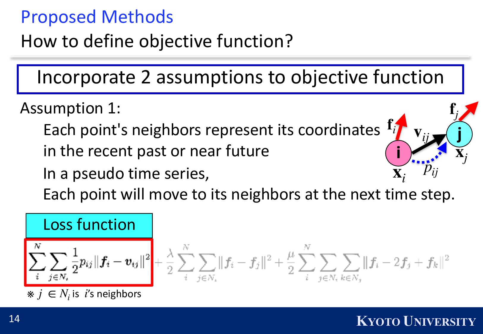
Incorporate 2 assumptions to objective function Assumption 1: In a pseudo time series, Each point will move to its neighbors at the next time step. Each point's neighbors represent its coordinates in the recent past or near future Loss function ※ is ’s neighbors j ∈ Ni i fi i j xi xj vij pij fj
Incorporate 2 assumptions to objective function Assumption 2: The vector field is smooth , and neighboring point clouds have similar trajectory vectors Acceleration smoothing Velocity smoothing ※ is ’s neighbors, is ’s neighbors j ∈ Ni i k ∈ Nj j fi i j k xi xj xk fj fk
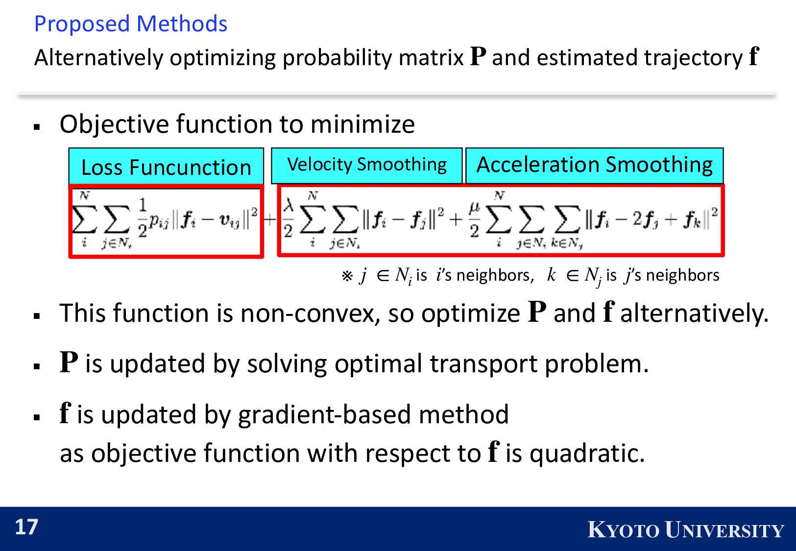
estimated trajectory P f ▪ Objective function to minimize ▪ This function is non-convex, so optimize and alternatively. ▪ is transition probability matrix where ▪ is estimated trajectory estimated by neural network . P f P Pij = pij f fθ Acceleration Smoothing Velocity Smoothing ※ is ’s neighbors, is ’s neighbors j ∈ Ni i k ∈ Nj j Loss Funcunction
estimated trajectory P f ▪ Objective function to minimize ▪ This function is non-convex, so optimize and alternatively. ▪ is updated by solving optimal transport problem. ▪ is updated by gradient-based method as objective function with respect to is quadratic. P f P f f Acceleration Smoothing Velocity Smoothing ※ is ’s neighbors, is ’s neighbors j ∈ Ni i k ∈ Nj j Loss Funcunction
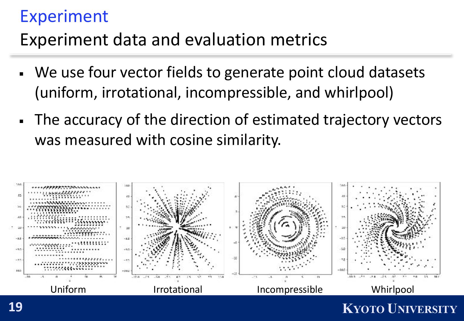
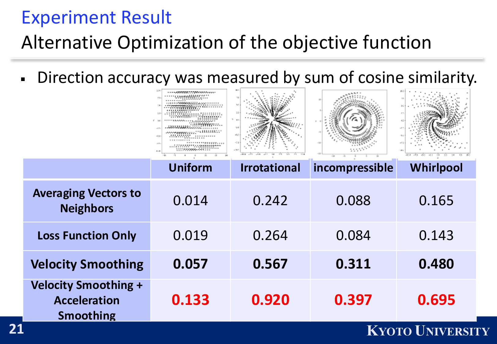
We use four vector fields to generate point cloud datasets (uniform, irrotational, incompressible, and whirlpool) ▪ The accuracy of the direction of estimated trajectory vectors was measured with cosine similarity. Uniform Irrotational Incompressible Whirlpool
function ▪ Direction accuracy was measured by sum of cosine similarity. Uniform Irrotational incompressible Whirlpool Averaging Vectors to Neighbors 0.014 0.242 0.088 0.165 Loss Function Only 0.019 0.264 0.084 0.143 Velocity Smoothing 0.057 0.567 0.311 0.480 Velocity Smoothing + Acceleration Smoothing 0.133 0.920 0.397 0.695
MLP(SNVF) ▪ Metric: RMSE between and RMSE considers both magnitude and direction of estimated trajectories ▪ Velocity smoothing works effectively for irrotational data and acceleration smoothing works for incompressible and whirlpool data. fi V(xi )
Single Pointcloud Snapshot ▪ In this study, we estimate trajectory of each point from a point cloud data with only coordinates at a single time. In other words, the motion of each point was restored from the coordinates of the motionless point cloud. ▪ In this research, we proposed a formulation of the problem set and devised an algorithm to solve it at the same time. ▪ Experimental results showed that two types of regularization terms, velocity smoothing and acceleration smoothing, significantly improve the accuracy of the estimation.
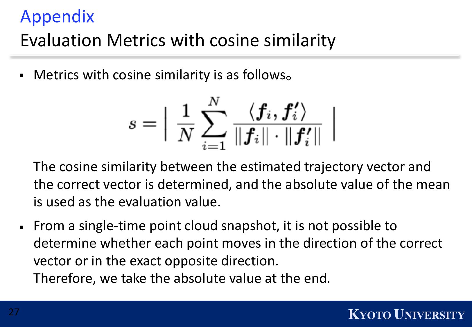
Metrics with cosine similarity is as followsɻ The cosine similarity between the estimated trajectory vector and the correct vector is determined, and the absolute value of the mean is used as the evaluation value. ▪ From a single-time point cloud snapshot, it is not possible to determine whether each point moves in the direction of the correct vector or in the exact opposite direction. Therefore, we take the absolute value at the end.
time series data are given ▪ Assume that point cloud data time series(t = 0, … T) are given ▪ Predict trajectory with observed trajectory (µ0, . . . , µT)
time series data are given ▪ Use formula called JKO flows ▪ : a probability distribution, : a time step parameter ▪ : Wasserstein distance ▪ is an energy function and it represents time evolution ρ τ W2 2 (μ, ν) J
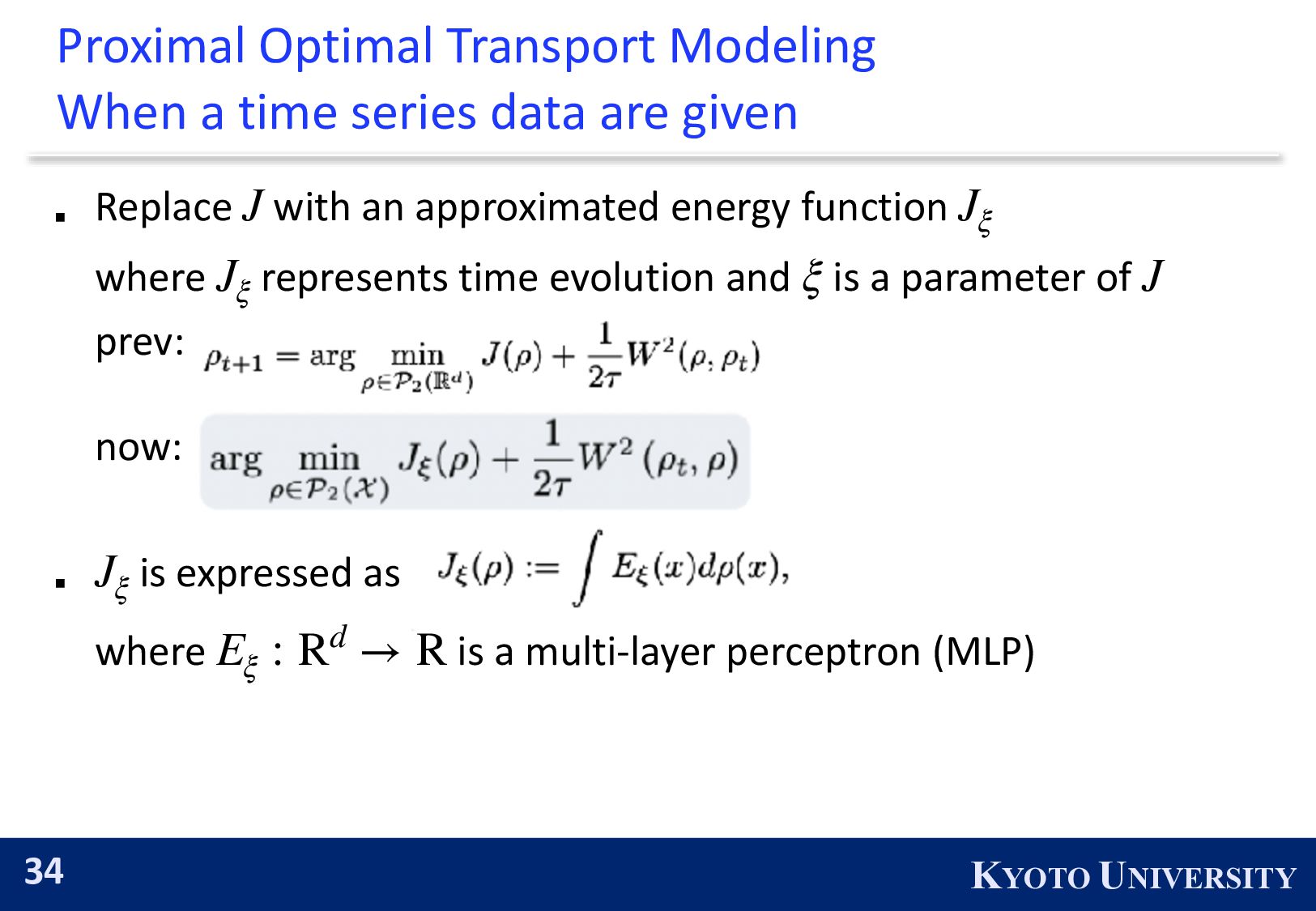
time series data are given ▪ Replace with an approximated energy function where represents time evolution and is a parameter of prev: now: ▪ is expressed as where is a multi-layer perceptron (MLP) J Jξ Jξ ξ J Jξ Eξ : Rd → R
time series data are given ▪ is a multi-layer perceptron (MLP) ▪ Datasets are given ▪ Loss is written as ▪ Loss is calculated with the help of Sinkhorn algorithm Eξ : Rd → R D = {{μ0 t }T t=0 , ⋯, {μN t }T t=0 }
average of cell population ▪ With traditional methods: each cell’s state is estimated from an average of cell population ▪ The cell population can only be monitored with periodic snapshots of a few sampled particles in various states. Cell Population
inference tries to obtain “pseudotime” series from members of cell population in order to analyze each cell more precisely Cell Population “Pseudotime” axis
trajectory inference, there are numerous methods, but they are roughly categorized in two main methods. ▪ One method is dimensionality reduction (such as PCA), and project cell population onto “pseudotime” axis with the help of principle components.
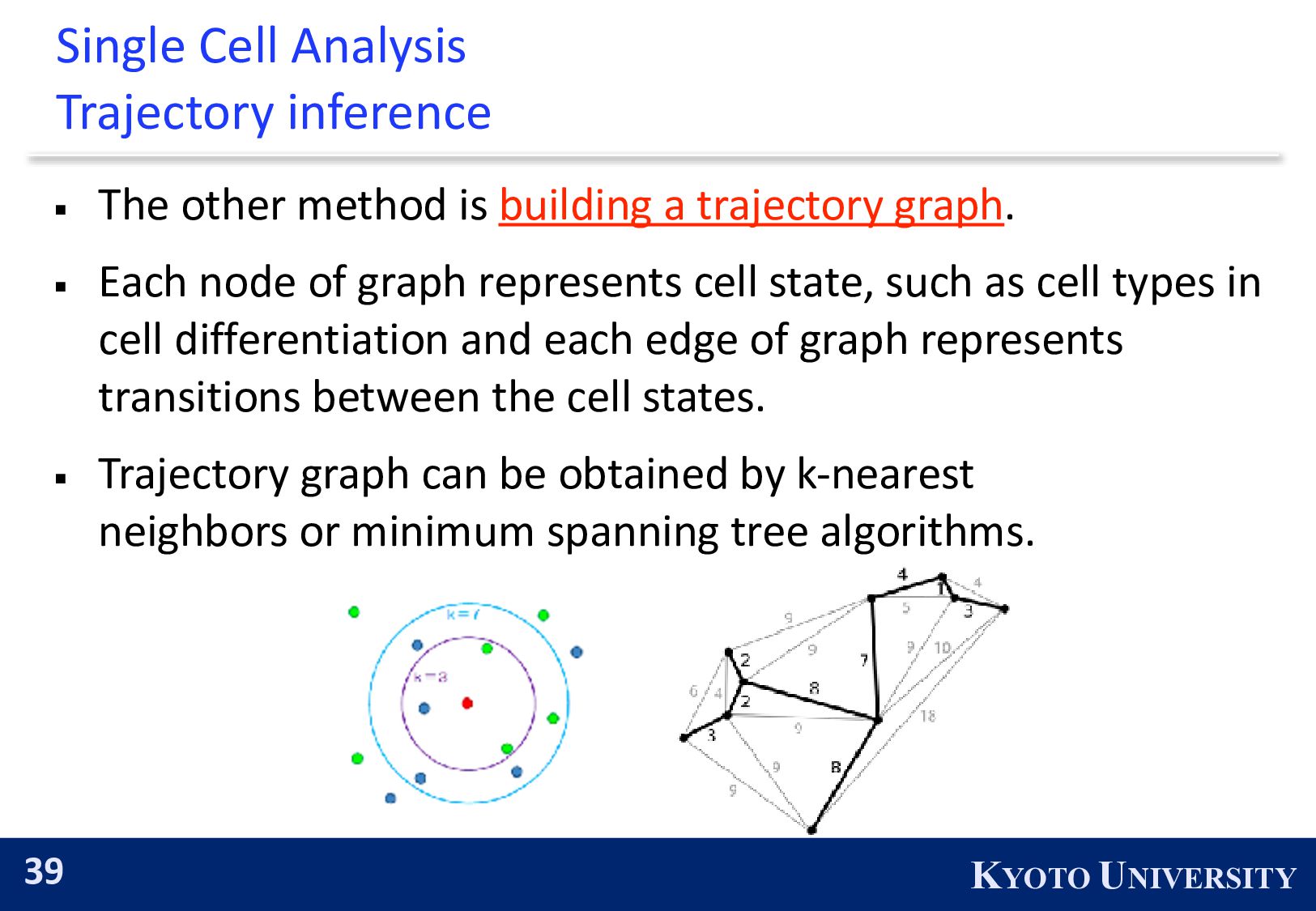
other method is building a trajectory graph. ▪ Each node of graph represents cell state, such as cell types in cell differentiation and each edge of graph represents transitions between the cell states. ▪ Trajectory graph can be obtained by k-nearest neighbors or minimum spanning tree algorithms.


 waxayuzu0
 deanohume
 tammyeverts
 skipperchong
 retrage
 joshbly
 bluesmoon
 destraynor
 cassininazir
 uxyall
 codingconduct
 csswizardry
 eileencodes