Call-by-name, call-by-value and the λ-calculus

Transcript

1. CALL-BY-NAME, CALL-BY-VALUE AND THE λ-CALCULUS G.D.PLOTKIN, 1975 Yudai Urabe September 24, 2025 Yudai Urabe (Plotkin,1975) 1 / 29
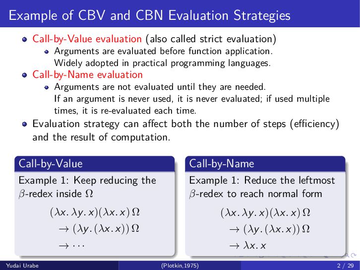
2. Example of CBV and CBN Evaluation Strategies Call-by-Value evaluation (also called strict evaluation) Arguments are evaluated before function application. Widely adopted in practical programming languages. Call-by-Name evaluation Arguments are not evaluated until they are needed. If an argument is never used, it is never evaluated; if used multiple times, it is re-evaluated each time. Evaluation strategy can affect both the number of steps (efficiency) and the result of computation. Call-by-Value Example 1: Keep reducing the β-redex inside Ω (λx. λy. x)(λx. x) Ω → (λy. (λx. x)) Ω → · · · Call-by-Name Example 1: Reduce the leftmost β-redex to reach normal form (λx. λy. x)(λx. x) Ω → (λy. (λx. x)) Ω → λx. x Yudai Urabe (Plotkin,1975) 2 / 29
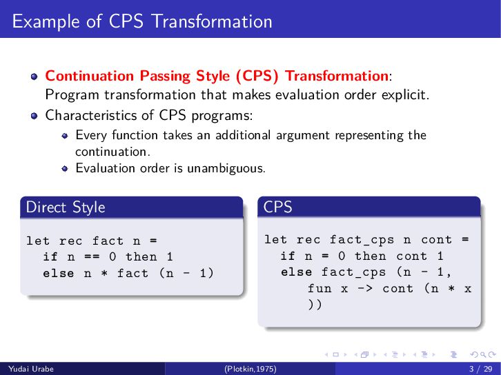
3. Example of CPS Transformation Continuation Passing Style (CPS) Transformation: Program transformation that makes evaluation order explicit. Characteristics of CPS programs: Every function takes an additional argument representing the continuation. Evaluation order is unambiguous. Direct Style let rec fact n = if n == 0 then 1 else n * fact (n - 1) CPS let rec fact_cps n cont = if n = 0 then cont 1 else fact_cps (n - 1, fun x -> cont (n * x )) Yudai Urabe (Plotkin,1975) 3 / 29
4. Comparing Execution in Direct Style and CPS To execute CPS expressions, we pass the identity function. As shown below, evaluation in DS and CPS yields the same result (to be proved later). DS: Execution of fact(3) fact(3) = 3 * fact(2) = 3 * (2 * fact(1)) = 3 * (2 * (1 * fact(0))) = 3 * (2 * (1 * 1)) = 6 CPS: Execution of factcps (3, id) fact_cps(3, id) = fact_cps(2, fun x -> id (3 * x)) = fact_cps(1, fun x2 -> id(3 * (2 * x2))) = fact_cps(0, fun x3 -> id(3 * (2 * (1 * x3 )))) = id(3 * (2 * (1 * 1))) = 6 (Simplified for readability.) Yudai Urabe (Plotkin,1975) 4 / 29
5. §6 Proof Sketch (Simulating CBV in CBN) Pure λ-Calculus M Source Language CBN–CPS M Target Language Value Value EvalV EvalN Thm. 6.2 Ψ Thm. 6.3 CPS Trans. (p.147) Cor. 6.2 EvalV Thm. 6.1 Yudai Urabe (Plotkin,1975) 5 / 29
6. Definitions (”Constants” removed compared to the original paper)
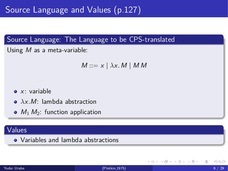
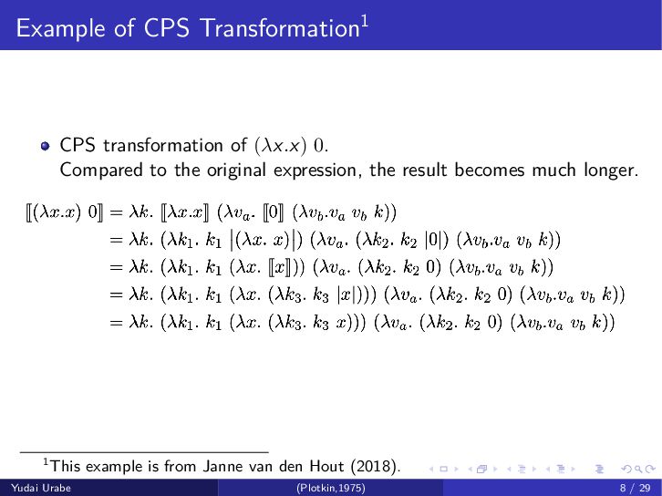
7. Source Language and Values (p.127) Source Language: The Language to be CPS-translated Using M as a meta-variable: M ::= x | λx. M | M M x: variable λx.M: lambda abstraction M1 M2: function application Values Variables and lambda abstractions Yudai Urabe (Plotkin,1975) 6 / 29
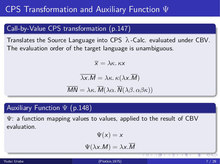
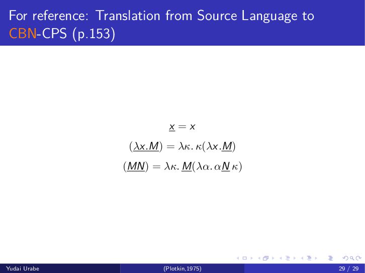
8. CPS Transformation and Auxiliary Function Ψ Call-by-Value CPS transformation (p.147) Translates the Source Language into CPS λ-Calc. evaluated under CBV. The evaluation order of the target language is unambiguous. x = λκ. κx λx.M = λκ. κ(λx.M) MN = λκ. M(λα. N(λβ. αβκ)) Auxiliary Function Ψ (p.148) Ψ: a function mapping values to values, applied to the result of CBV evaluation. Ψ(x) = x Ψ(λx.M) = λx.M Yudai Urabe (Plotkin,1975) 7 / 29
9. Example of CPS Transformation1 CPS transformation of (λx.x) 0. Compared to the original expression, the result becomes much longer. 1This example is from Janne van den Hout (2018). Yudai Urabe (Plotkin,1975) 8 / 29
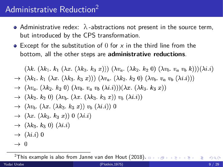
10. Administrative Reduction2 Administrative redex: λ-abstractions not present in the source term, but introduced by the CPS transformation. Except for the substitution of 0 for x in the third line from the bottom, all the other steps are administrative reductions. 2This example is also from Janne van den Hout (2018). Yudai Urabe (Plotkin,1975) 9 / 29
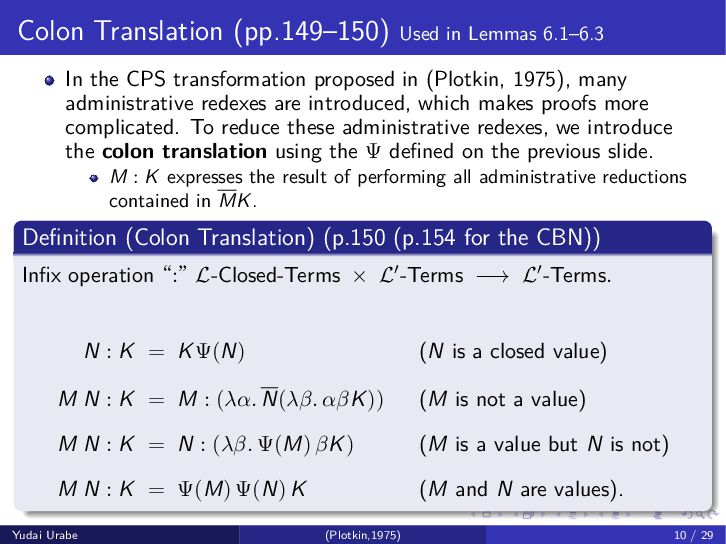
11. Colon Translation (pp.149–150) Used in Lemmas 6.1–6.3 In the CPS transformation proposed in (Plotkin, 1975), many administrative redexes are introduced, which makes proofs more complicated. To reduce these administrative redexes, we introduce the colon translation using the Ψ defined on the previous slide. M : K expresses the result of performing all administrative reductions contained in MK. Definition (Colon Translation) (p.150 (p.154 for the CBN)) Infix operation “:” L-Closed-Terms × L -Terms −→ L -Terms. N : K = KΨ(N) (N is a closed value) M N : K = M : (λα. N(λβ. αβK)) (M is not a value) M N : K = N : (λβ. Ψ(M) βK) (M is a value but N is not) M N : K = Ψ(M) Ψ(N) K (M and N are values). Yudai Urabe (Plotkin,1975) 10 / 29
12. Proof of Thm. 6.2 (CBV can be simulated by CBN)
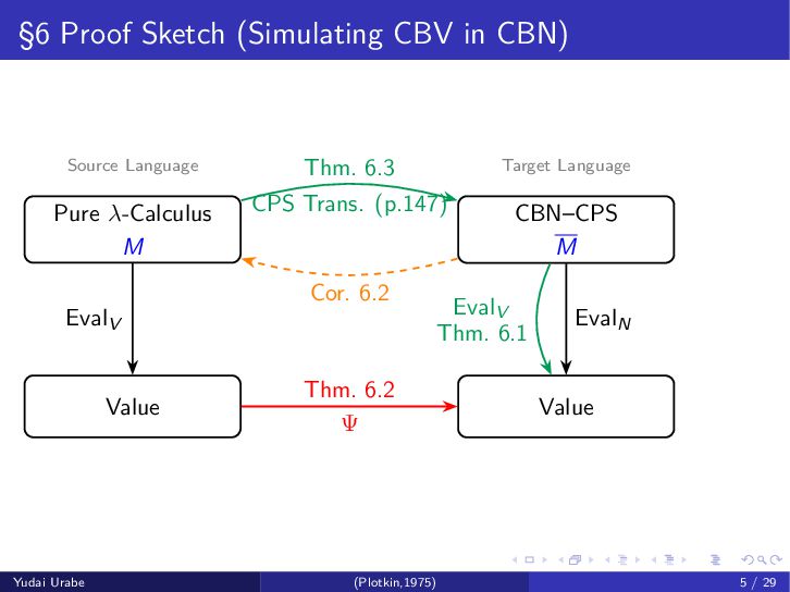
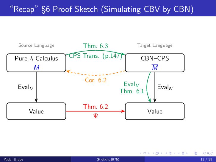
13. “Recap” §6 Proof Sketch (Simulating CBV by CBN) Pure λ-Calculus M Source Language CBN–CPS M Target Language Value Value EvalV EvalN Thm. 6.2 Ψ Thm. 6.3 CPS Trans. (p.147) Cor. 6.2 EvalV Thm. 6.1 Yudai Urabe (Plotkin,1975) 11 / 29
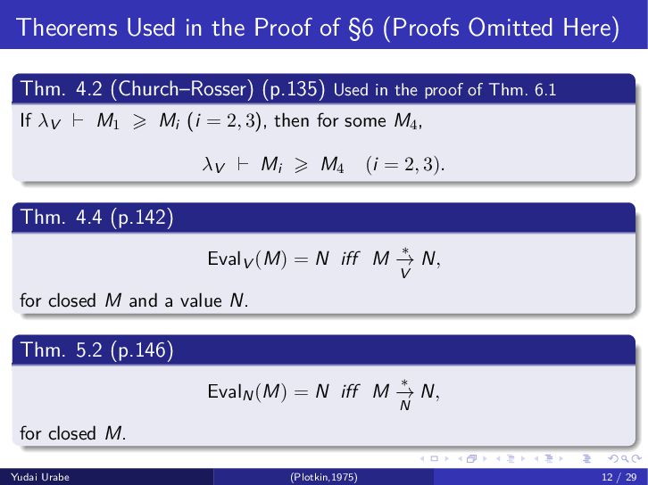
14. Theorems Used in the Proof of §6 (Proofs Omitted Here) Thm. 4.2 (Church–Rosser) (p.135) Used in the proof of Thm. 6.1 If λV M1 Mi (i = 2, 3), then for some M4, λV Mi M4 (i = 2, 3). Thm. 4.4 (p.142) EvalV (M) = N iff M ∗ → V N, for closed M and a value N. Thm. 5.2 (p.146) EvalN(M) = N iff M ∗ → N N, for closed M. Yudai Urabe (Plotkin,1975) 12 / 29
15. Three Main Theorems in This Paper Thm. 6.1 (Indifference) EvalN(M(λx.x)) = EvalV (M(λx.x)). for any program M. Yudai Urabe (Plotkin,1975) 13 / 29
16. Three Main Theorems in This Paper Thm. 6.1 (Indifference) EvalN(M(λx.x)) = EvalV (M(λx.x)). for any program M. Thm. 6.2 (Simulation) Ψ(EvalV (M)) = EvalN(M(λx.x)), for any program M. Yudai Urabe (Plotkin,1975) 13 / 29
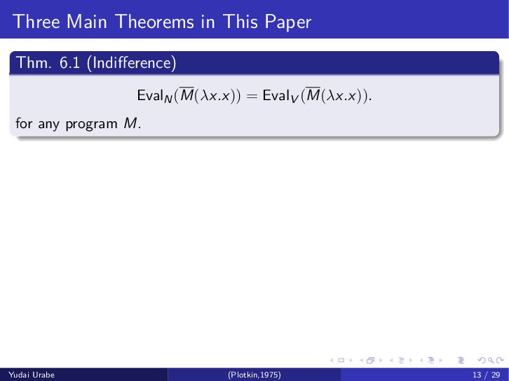
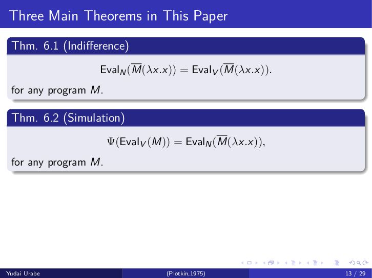
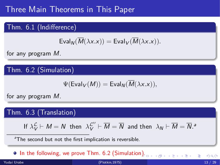
17. Three Main Theorems in This Paper Thm. 6.1 (Indifference) EvalN(M(λx.x)) = EvalV (M(λx.x)). for any program M. Thm. 6.2 (Simulation) Ψ(EvalV (M)) = EvalN(M(λx.x)), for any program M. Thm. 6.3 (Translation) If λL V M = N then λL V M = N and then λN M = N.a aThe second but not the first implication is reversible. In the following, we prove Thm. 6.2 (Simulation). Yudai Urabe (Plotkin,1975) 13 / 29
18. (1) Lemmas 6.1 and 6.2 (pp.149–150) Lem. 6.1 [Ψ(N)/x] M = [N/x]M (if N is a value). Lem. 6.2 If K is a closed value then MK + − → M : K, for any term M. Yudai Urabe (Plotkin,1975) 14 / 29
19. (2) Lemma 6.3 Lem. 6.3 M → V N ⇒ M : K + − → N : K (if K is a closed value and M, N are terms). Yudai Urabe (Plotkin,1975) 15 / 29
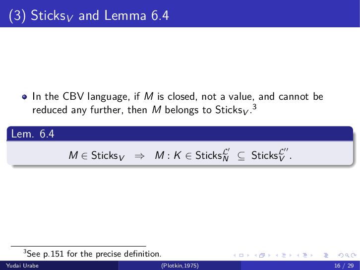
20. (3) SticksV and Lemma 6.4 In the CBV language, if M is closed, not a value, and cannot be reduced any further, then M belongs to SticksV .3 Lem. 6.4 M ∈ SticksV ⇒ M : K ∈ SticksL N ⊆ SticksL V . 3See p.151 for the precise definition. Yudai Urabe (Plotkin,1975) 16 / 29
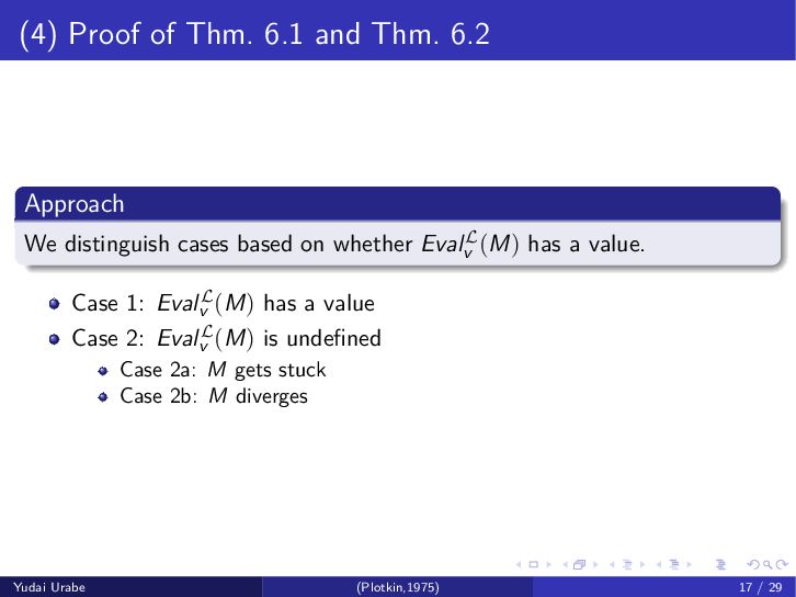
21. (4) Proof of Thm. 6.1 and Thm. 6.2 Approach We distinguish cases based on whether EvalL v (M) has a value. Case 1: EvalL v (M) has a value Case 2: EvalL v (M) is undefined Case 2a: M gets stuck Case 2b: M diverges Yudai Urabe (Plotkin,1975) 17 / 29
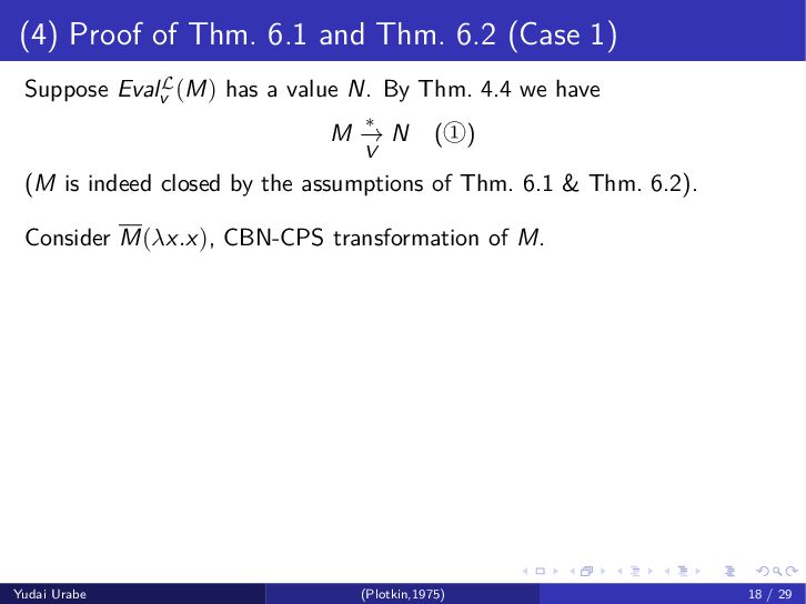
22. (4) Proof of Thm. 6.1 and Thm. 6.2 (Case 1) Suppose EvalL v (M) has a value N. By Thm. 4.4 we have M ∗ − → V N (①) (M is indeed closed by the assumptions of Thm. 6.1 & Thm. 6.2). Consider M(λx.x), CBN-CPS transformation of M. Yudai Urabe (Plotkin,1975) 18 / 29
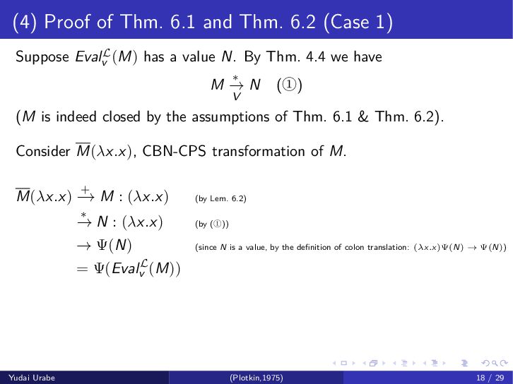
23. (4) Proof of Thm. 6.1 and Thm. 6.2 (Case 1) Suppose EvalL v (M) has a value N. By Thm. 4.4 we have M ∗ − → V N (①) (M is indeed closed by the assumptions of Thm. 6.1 & Thm. 6.2). Consider M(λx.x), CBN-CPS transformation of M. M(λx.x) + − → M : (λx.x) (by Lem. 6.2) ∗ − → N : (λx.x) (by (①)) → Ψ(N) (since N is a value, by the definition of colon translation: (λx.x)Ψ(N) → Ψ(N)) = Ψ(EvalL v (M)) Yudai Urabe (Plotkin,1975) 18 / 29
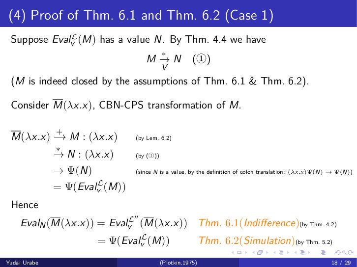
24. (4) Proof of Thm. 6.1 and Thm. 6.2 (Case 1) Suppose EvalL v (M) has a value N. By Thm. 4.4 we have M ∗ − → V N (①) (M is indeed closed by the assumptions of Thm. 6.1 & Thm. 6.2). Consider M(λx.x), CBN-CPS transformation of M. M(λx.x) + − → M : (λx.x) (by Lem. 6.2) ∗ − → N : (λx.x) (by (①)) → Ψ(N) (since N is a value, by the definition of colon translation: (λx.x)Ψ(N) → Ψ(N)) = Ψ(EvalL v (M)) Hence EvalN(M(λx.x)) = EvalL v (M(λx.x)) Thm. 6.1(Indifference)(by Thm. 4.2) = Ψ(EvalL v (M)) Thm. 6.2(Simulation)(by Thm. 5.2) Yudai Urabe (Plotkin,1975) 18 / 29
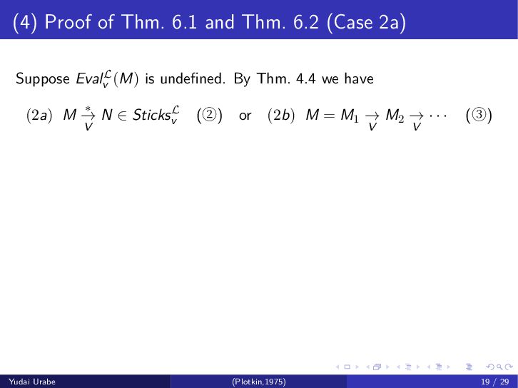
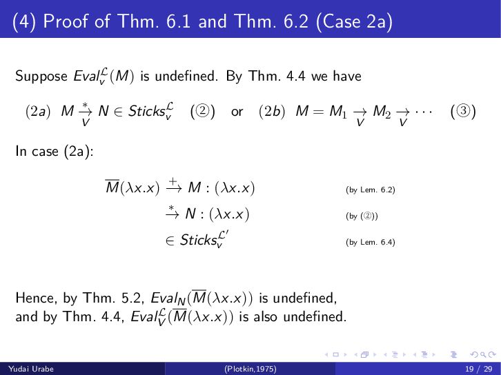
25. (4) Proof of Thm. 6.1 and Thm. 6.2 (Case 2a) Suppose EvalL v (M) is undefined. By Thm. 4.4 we have (2a) M ∗ − → V N ∈ SticksL v (②) or (2b) M = M1 → V M2 → V · · · (③) Yudai Urabe (Plotkin,1975) 19 / 29
26. (4) Proof of Thm. 6.1 and Thm. 6.2 (Case 2a) Suppose EvalL v (M) is undefined. By Thm. 4.4 we have (2a) M ∗ − → V N ∈ SticksL v (②) or (2b) M = M1 → V M2 → V · · · (③) In case (2a): M(λx.x) + − → M : (λx.x) (by Lem. 6.2) ∗ − → N : (λx.x) (by (②)) ∈ SticksL v (by Lem. 6.4) Hence, by Thm. 5.2, EvalN(M(λx.x)) is undefined, and by Thm. 4.4, EvalL V (M(λx.x)) is also undefined. Yudai Urabe (Plotkin,1975) 19 / 29
27. (4) Proof of Thm. 6.1 and Thm. 6.2 (Case 2b) In case (2b): M(λx.x) + − → M : (λx.x) (by Lem. 6.2) = M1 : (λx.x) (by (③)) + − → M : (λx.x) (by Lem. 6.2) + − → · · · Hence both EvalN(M(λx.x)) and EvalL V (M(λx.x)) diverge. Yudai Urabe (Plotkin,1975) 20 / 29
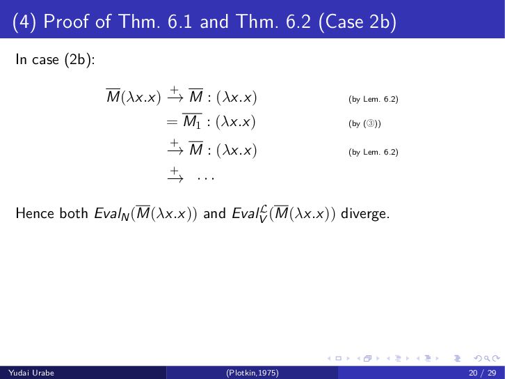
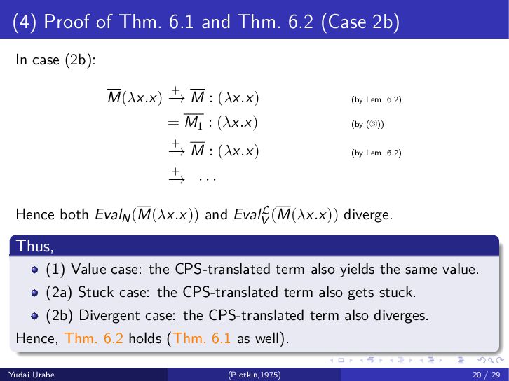
28. (4) Proof of Thm. 6.1 and Thm. 6.2 (Case 2b) In case (2b): M(λx.x) + − → M : (λx.x) (by Lem. 6.2) = M1 : (λx.x) (by (③)) + − → M : (λx.x) (by Lem. 6.2) + − → · · · Hence both EvalN(M(λx.x)) and EvalL V (M(λx.x)) diverge. Thus, (1) Value case: the CPS-translated term also yields the same value. (2a) Stuck case: the CPS-translated term also gets stuck. (2b) Divergent case: the CPS-translated term also diverges. Hence, Thm. 6.2 holds (Thm. 6.1 as well). Yudai Urabe (Plotkin,1975) 20 / 29
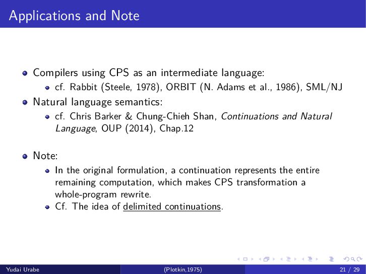
29. Applications and Note Compilers using CPS as an intermediate language: cf. Rabbit (Steele, 1978), ORBIT (N. Adams et al., 1986), SML/NJ Natural language semantics: cf. Chris Barker & Chung-Chieh Shan, Continuations and Natural Language, OUP (2014), Chap.12 Note: In the original formulation, a continuation represents the entire remaining computation, which makes CPS transformation a whole-program rewrite. Cf. The idea of delimited continuations. Yudai Urabe (Plotkin,1975) 21 / 29
30. Related Works (1) John C. Reynolds. 1972. Definitional interpreters for higher-order programming languages. In Proc. ACM Annual Conference - Vol.2, pp.717–740. Christopher Strachey and Christopher P. Wadsworth. 1974. Continuations: A mathematical semantics for handling full jumps. Reprinted in Higher-Order and Symbolic Computation (2000). Gordon D. Plotkin. 1975. Call-by-name, call-by-value and the λ-calculus.Theoretical Computer Science 1(2):125 – 159. Janne van den Hout. 2018. Continuations in functional programming languages. BSc thesis, Radboud University. §4.2 gives a detailed account of CPS and colon translation, with examples (Ex.4.2.1, Ex.4.2.2). Gordon D. Plotkin. 2004. The origins of structural operational semantics. The Journal of Logic and Algebraic Programming, 60–61:3–15. Yudai Urabe (Plotkin,1975) 22 / 29
31. Related Works (2) Cormac Flanagan, Amr Sabry, Bruce F. Duba, and Matthias Felleisen. The Essence of Compiling with Continuations. In PLDI’ 93, pp.237–247. Introduced ANF. Olivier Danvy and Andrzej Filinski. 1992. Representing Control: A Study of the CPS Transformation. Mathematical Structures in Computer Science, 2(4):361–391. Olivier Danvy and Lasse R. Nielsen. 2002. A First-Order One-Pass CPS Transformation. In FoSSaCS, LNCS 2303, pp.98–113. Springer. Defines a CPS/colon translation eliminating more administrative redexes than Plotkin’s original colon translation. Olivier Danvy. 2004. On Evaluation Contexts, Continuations, and the Rest of Computation. In Proc. Fourth ACM SIGPLAN Workshop on Continuations, Technical Report CSR-04-1, School of Computer Science, University of Birmingham, pp.13–23. Encyclopedia of Theoretical Computer Science (in Japanese). Yudai Urabe (Plotkin,1975) 23 / 29
32. Related Works (3): Applications of CPS Guy L. Steele. 1978. Rabbit: A Compiler for Scheme. Technical Report, MIT. Norman Adams, David Kranz, Richard Kelsey, Jonathan Rees, Paul Hudak, and James Philbin. 1986. ORBIT: An Optimizing Compiler for Scheme. SIGPLAN Not. 21(7):219–233. Andrew W. Appel. 1992. Compiling with Continuations. Cambridge University Press. Chris Barker. 2002. Continuations and the Nature of Quantification. Natural Language Semantics 10:211–242. Chris Barker & Chung-Chieh Shan. 2014. Continuations and Natural Language. Oxford University Press. Masaya Taniguchi. 2022. Unprovability of Continuation-Passing Style Transformation in Lambek Calculus. ESSLLI Student Session, Galway. Yudai Urabe (Plotkin,1975) 24 / 29
33. Appendix
34. Quick Reference of Definitions (partial) normal form (p.126, p.142) value (p.127) substitution (p.127) + − → and ∗ − → (p.128) EvalV (p.129, p.130, SECD machine semantics), evalV (p.130) EvalN (p.145), evalN (not used) → V (p.136), → N (p.146) context/hole (p.144) ≈V (p.144), ≈N (p.147) continuation (p.147, with three different usages) Yudai Urabe (Plotkin,1975) 25 / 29
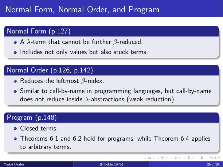
35. Normal Form, Normal Order, and Program Normal Form (p.127) A λ-term that cannot be further β-reduced. Includes not only values but also stuck terms. Normal Order (p.126, p.142) Reduces the leftmost β-redex. Similar to call-by-name in programming languages, but call-by-name does not reduce inside λ-abstractions (weak reduction). Program (p.148) Closed terms. Theorems 6.1 and 6.2 hold for programs, while Theorem 6.4 applies to arbitrary terms. Yudai Urabe (Plotkin,1975) 26 / 29
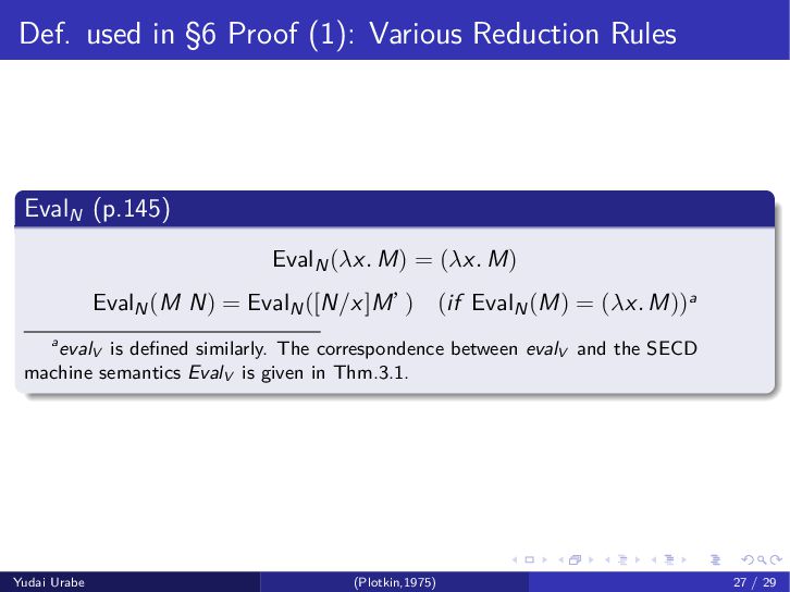
36. Def. used in §6 Proof (1): Various Reduction Rules EvalN (p.145) EvalN(λx. M) = (λx. M) EvalN(M N) = EvalN([N/x]M’ ) (if EvalN(M) = (λx. M))a aevalV is defined similarly. The correspondence between evalV and the SECD machine semantics EvalV is given in Thm.3.1. Yudai Urabe (Plotkin,1975) 27 / 29
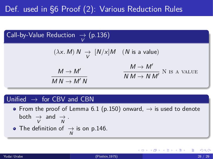
37. Def. used in §6 Proof (2): Various Reduction Rules Call-by-Value Reduction → V (p.136) (λx. M) N → V [N/x]M (N is a value) M → M M N → M N M → M N M → N M N is a value Unified → for CBV and CBN From the proof of Lemma 6.1 (p.150) onward, → is used to denote both → V and → N . The definition of → N is on p.146. Yudai Urabe (Plotkin,1975) 28 / 29
38. For reference: Translation from Source Language to CBN-CPS (p.153) x = x (λx.M) = λκ. κ(λx.M) (MN) = λκ. M(λα. αN κ) Yudai Urabe (Plotkin,1975) 29 / 29