Neutron Star Mass-Radius Constraints using Evolutionary Optimization

Pizza talk at the Anton Pannekoek Institute for Astronomy, University of Amsterdam, on 24 November 2016.

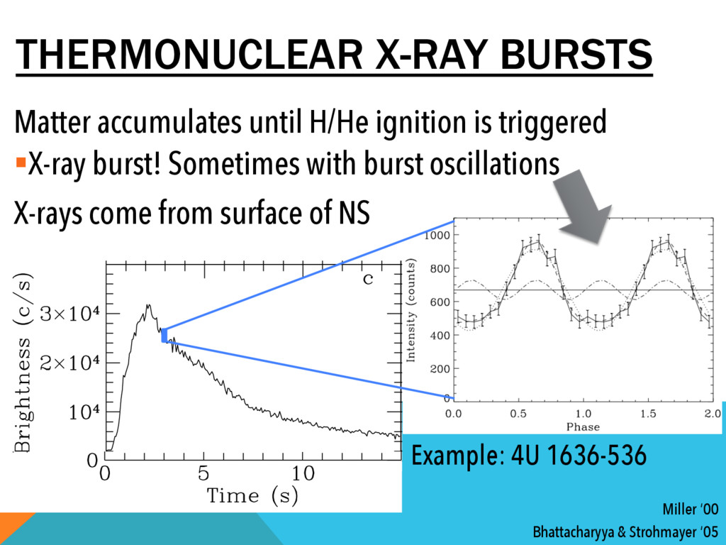
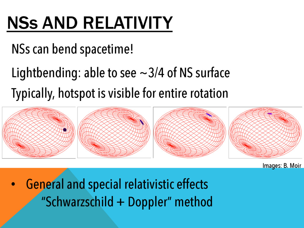
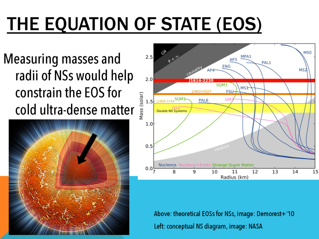
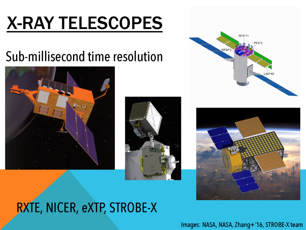
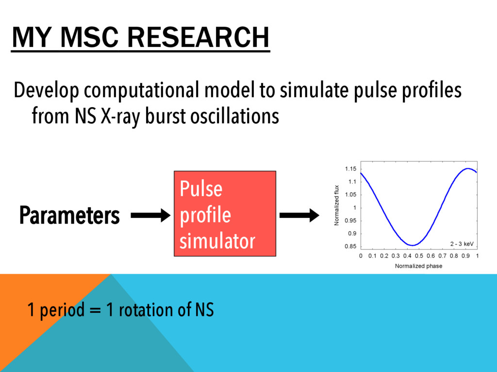
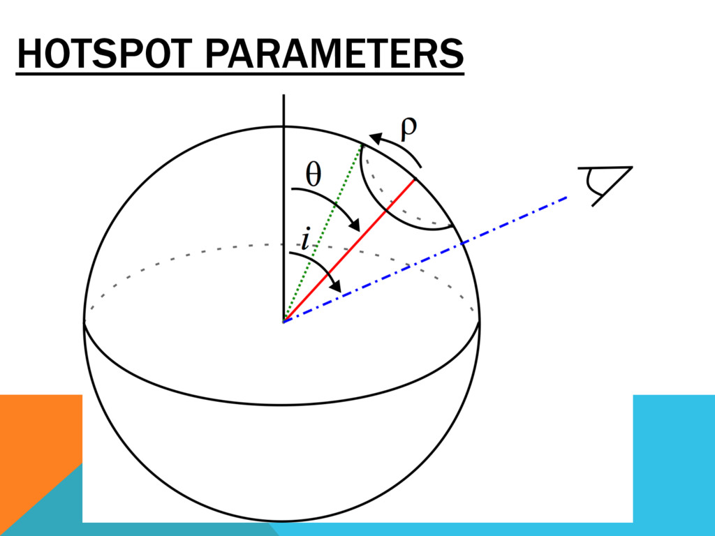
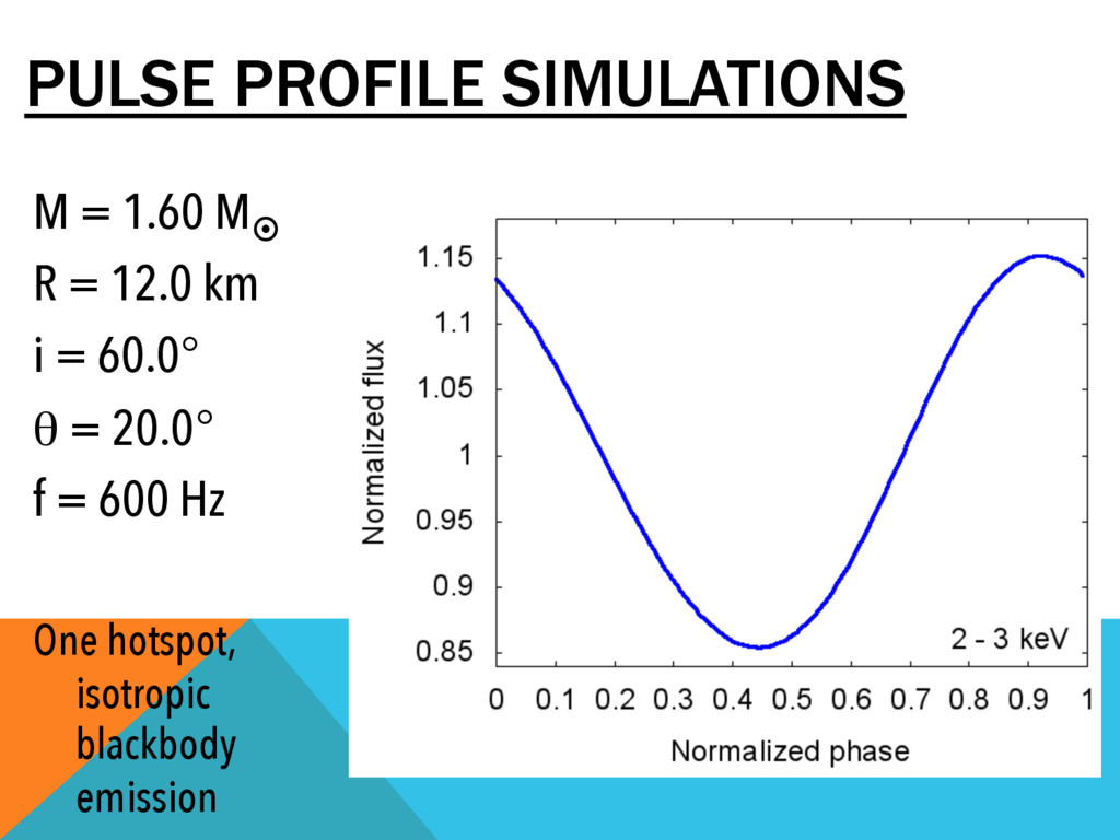
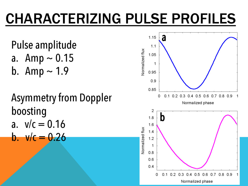
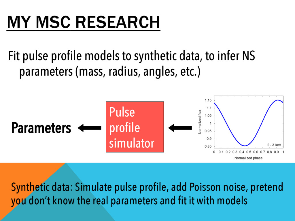
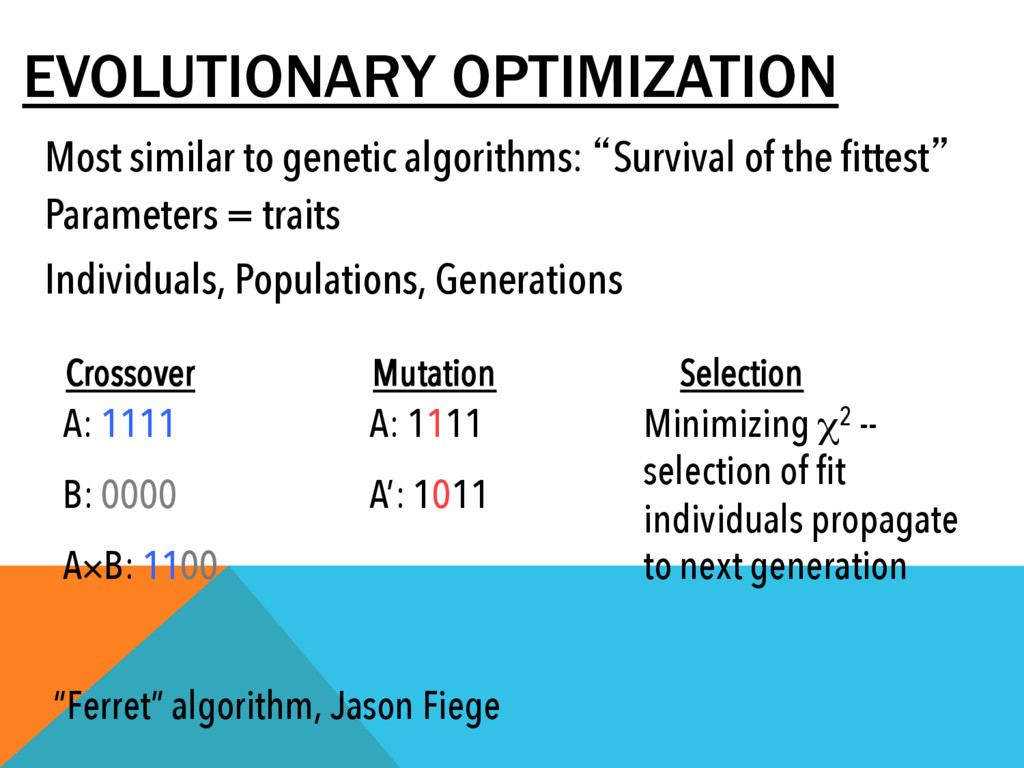
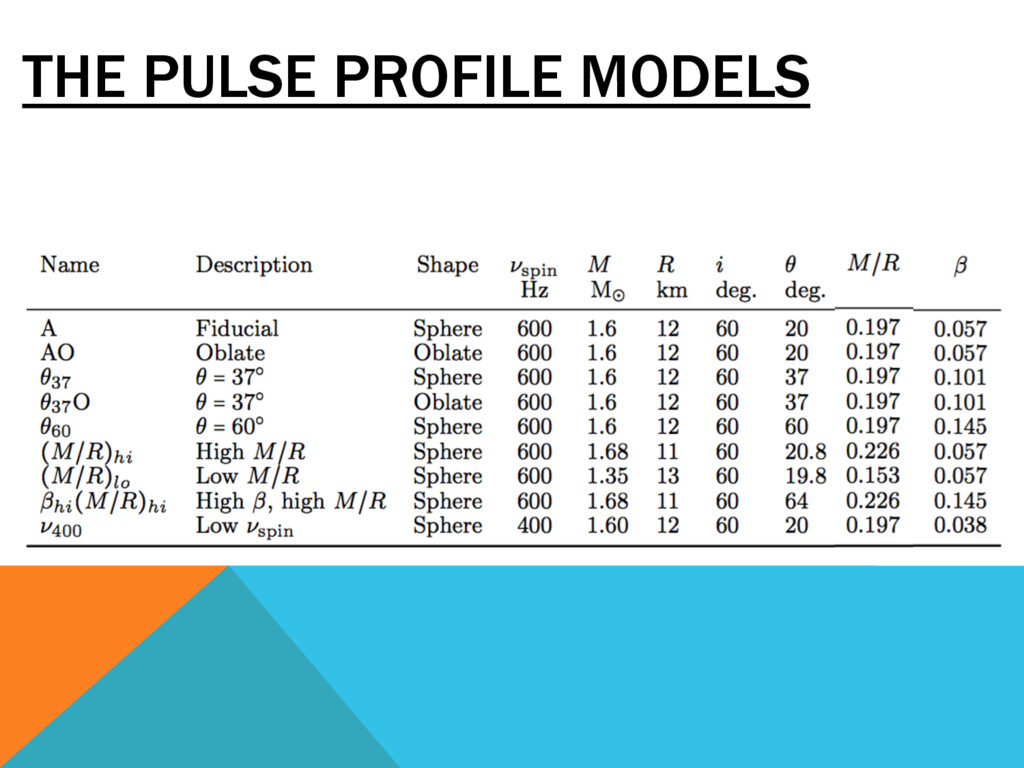
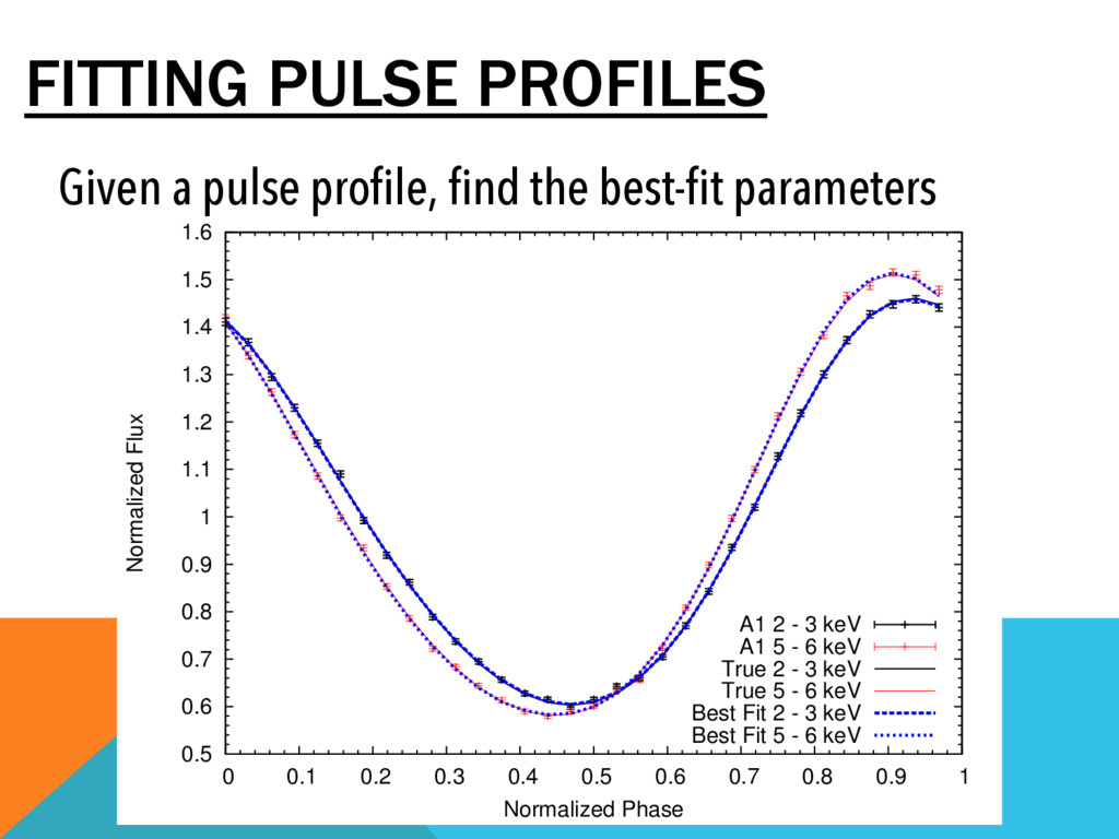
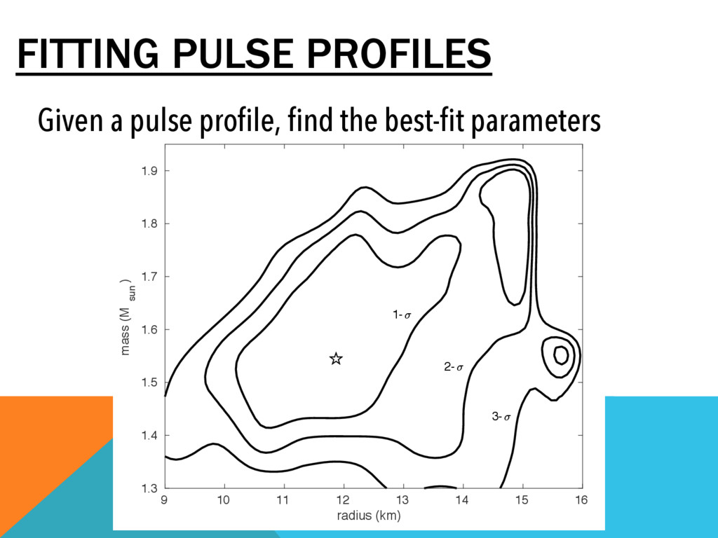
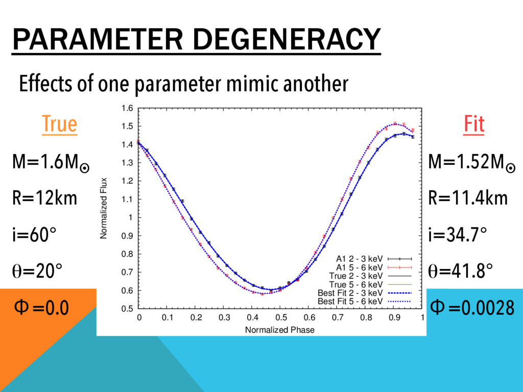
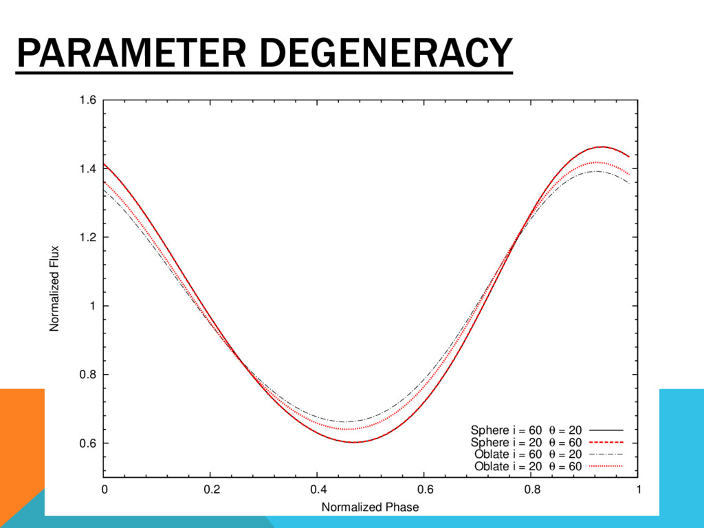
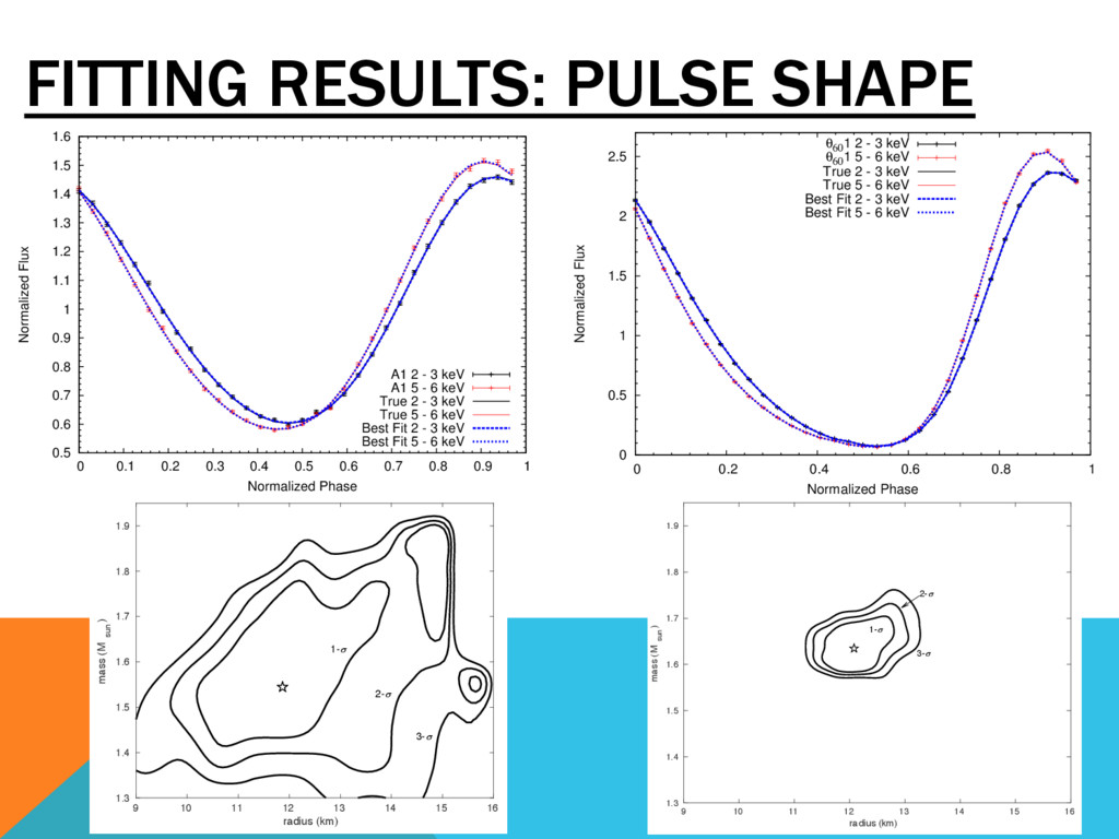
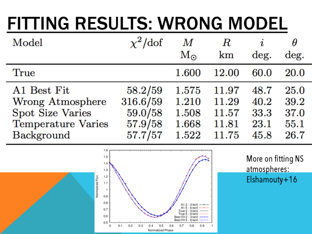
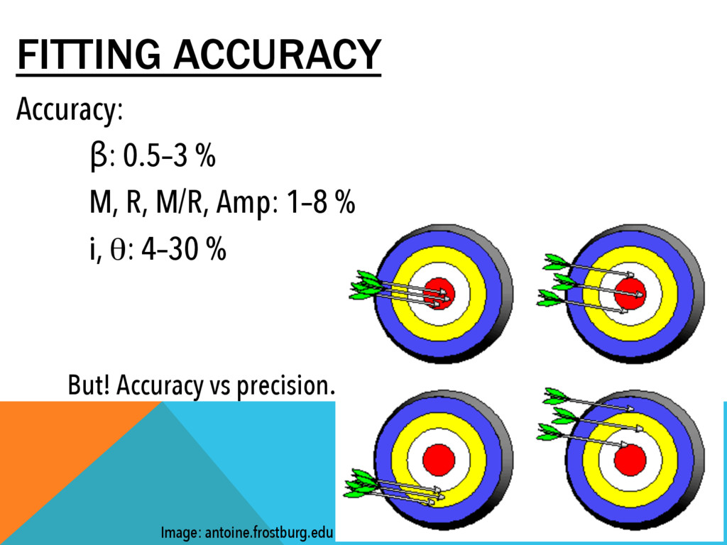
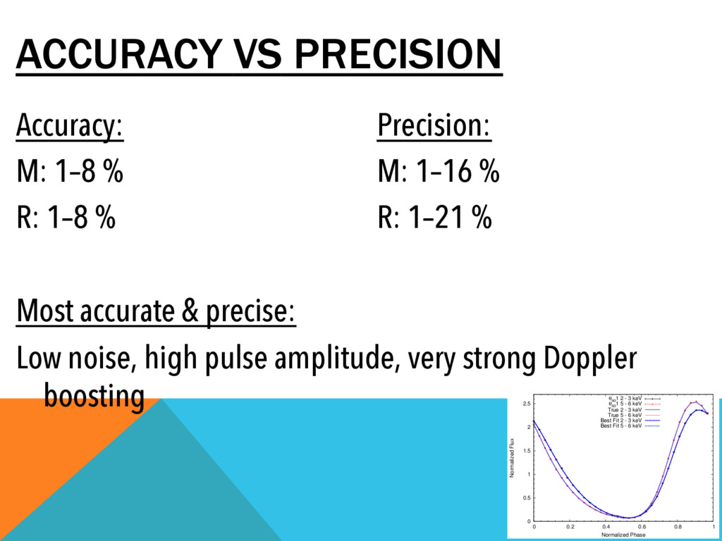
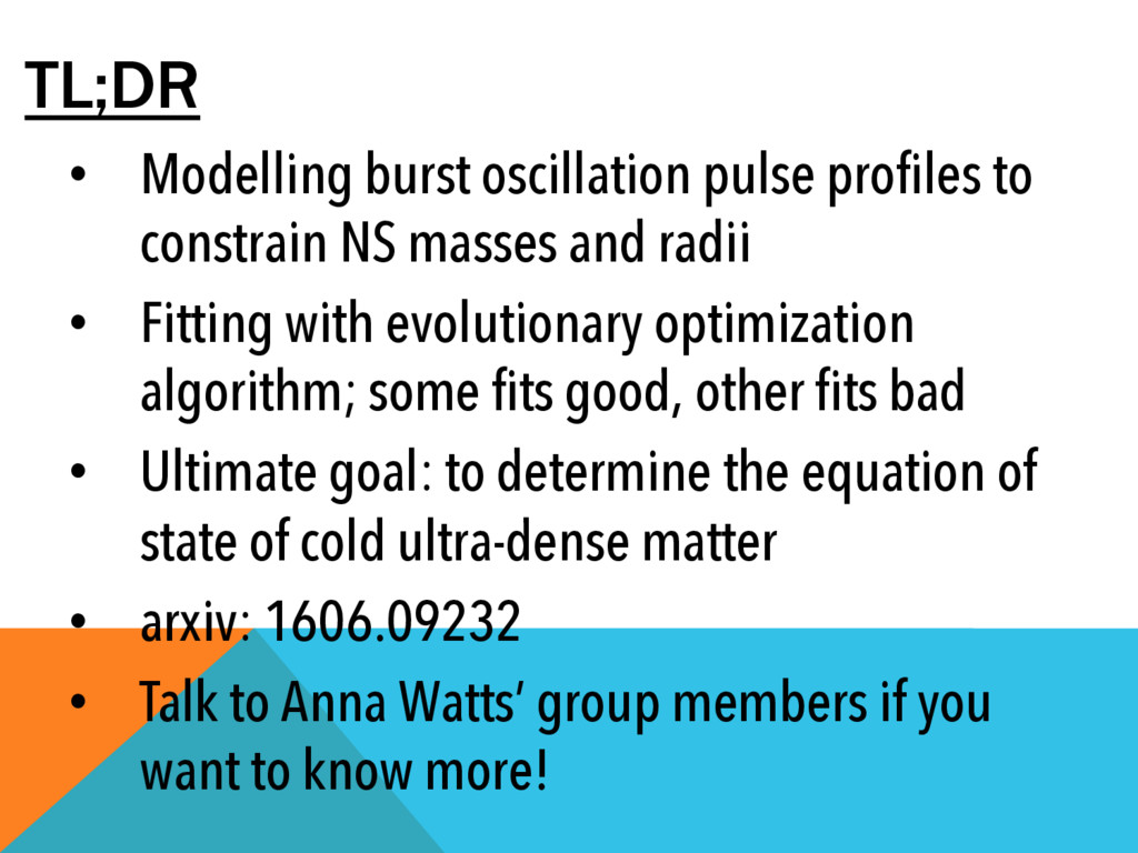
The equation of state of cold supra-nuclear-density matter, such as in neutron stars, is an open question in astrophysics. A promising method for constraining the neutron star equation of state is modelling pulse profiles of thermonuclear X-ray burst oscillations from hotspots on accreting neutron stars. The pulse profiles, constructed using spherical and oblate neutron star models, are comparable to what would be observed by a next- generation X-ray timing instrument like ASTROSAT, NICER, or STROBE-X. In this talk, we showcase the use of an evolutionary optimization algorithm to fit pulse profiles to determine the best-fit masses and radii. By fitting synthetic data, we assess how well the optimization algorithm can recover the input parameters. Multiple Poisson realizations of the synthetic pulse profiles were fitted with the Ferret algorithm to analyze both statistical and degeneracy-related uncertainty, and to explore how the goodness-of-fit depends on the input parameters. For the regions of parameter space sampled by our tests, the mass and radius fits were accurate to ≤ 5%, with respective uncertainties of ≤ 7% and ≤ 10%.

This is my MSc research; the paper published on it, recently accepted for publication in ApJ, is available here: https://ui.adsabs.harvard.edu/#abs/2016arXiv160609232S/abstract

Transcript

1. NEUTRON STAR MASS-RADIUS CONSTRAINTS USING EVOLUTIONARY OPTIMIZATION ABIGAIL STEVENS API PIZZA TALK, 24 NOV 2016 ARXIV: 1606.09232 J. FIEGE, D. LEAHY, S. MORSINK
2. Ultracompact remnant of a high- mass star ~8 - 20 M¤ R ~ 12 km M ~ 1.5 M¤ ρavg. ~ 1014 g/cm3 accelgravity ~ 1012 m/s2 B field ~ 108 - 1015 G fspin ~ 100s Hz NEUTRON STARS (NSs) Image: Google maps
3. NS primary < 1 M¤ companion Matter forms accretion disk around NS NS spins up to millisecond periods Image: NASA NSs IN LOW-MASS X-RAY BINARIES
4. Image: NASA Persistent pulsations and/or thermonuclear X-ray bursts ACCRETION ONTO HOTSPOTS
5. Matter accumulates until H/He ignition is triggered § X-ray burst! Sometimes with burst oscillations X-rays come from surface of NS Miller ‘00 Bhattacharyya & Strohmayer ‘05 Example: 4U 1636-536 THERMONUCLEAR X-RAY BURSTS
6. NSs can bend spacetime! Lightbending: able to see ~3/4 of NS surface Typically, hotspot is visible for entire rotation •  General and special relativistic effects “Schwarzschild + Doppler” method Images: B. Moir NSs AND RELATIVITY
7. Measuring masses and radii of NSs would help constrain the EOS for cold ultra-dense matter Above: theoretical EOSs for NSs, image: Demorest+’10 Left: conceptual NS diagram, image: NASA THE EQUATION OF STATE (EOS)
8. Sub-millisecond time resolution RXTE, NICER, eXTP, STROBE-X Images: NASA, NASA, Zhang+’16, STROBE-X team X-RAY TELESCOPES
9. Develop computational model to simulate pulse profiles from NS X-ray burst oscillations Pulse profile simulator Parameters 1 period = 1 rotation of NS MY MSC RESEARCH
10. HOTSPOT PARAMETERS
11. M = 1.60 M¤ R = 12.0 km i = 60.0° θ = 20.0° f = 600 Hz One hotspot, isotropic blackbody emission PULSE PROFILE SIMULATIONS
12. a b CHARACTERIZING PULSE PROFILES Pulse amplitude a.  Amp ~ 0.15 b.  Amp ~ 1.9 Asymmetry from Doppler boosting a. v/c = 0.16 b. v/c = 0.26
13. Fit pulse profile models to synthetic data, to infer NS parameters (mass, radius, angles, etc.) Pulse profile simulator Parameters Synthetic data: Simulate pulse profile, add Poisson noise, pretend you don’t know the real parameters and fit it with models MY MSC RESEARCH
14. Evolution makes weird things. OPTIMIZATION INSPIRATION: EVOLUTION! What kind of neutron star will we get? Nat. Geo. Kids YouTube/vlogbrothers Zuma press OTLibrary
15. Most similar to genetic algorithms: “Survival of the fittest” Parameters = traits Individuals, Populations, Generations Crossover Mutation Selection A: 1111 B: 0000 A×B: 1100 A: 1111 A’: 1011 Minimizing χ2 -- selection of fit individuals propagate to next generation “Ferret” algorithm, Jason Fiege EVOLUTIONARY OPTIMIZATION
16. THE PULSE PROFILE MODELS
17. Given a pulse profile, find the best-fit parameters FITTING PULSE PROFILES 0.5 0.6 0.7 0.8 0.9 1 1.1 1.2 1.3 1.4 1.5 1.6 0 0.1 0.2 0.3 0.4 0.5 0.6 0.7 0.8 0.9 1 Normalized Flux Normalized Phase A1 2 - 3 keV A1 5 - 6 keV True 2 - 3 keV True 5 - 6 keV Best Fit 2 - 3 keV Best Fit 5 - 6 keV
18. Given a pulse profile, find the best-fit parameters FITTING PULSE PROFILES Parameter Distribution 1-< 2-< 3-< 9 10 11 12 13 14 15 16 radius (km) 1.3 1.4 1.5 1.6 1.7 1.8 1.9 mass (M sun )
19. Effects of one parameter mimic another Fit M=1.52M¤ R=11.4km i=34.7° θ=41.8° Φ=0.0028 True M=1.6M¤ R=12km i=60° θ=20° Φ=0.0 PARAMETER DEGENERACY 0.5 0.6 0.7 0.8 0.9 1 1.1 1.2 1.3 1.4 1.5 1.6 0 0.1 0.2 0.3 0.4 0.5 0.6 0.7 0.8 0.9 1 Normalized Flux Normalized Phase A1 2 - 3 keV A1 5 - 6 keV True 2 - 3 keV True 5 - 6 keV Best Fit 2 - 3 keV Best Fit 5 - 6 keV
20. PARAMETER DEGENERACY 0.6 0.8 1 1.2 1.4 1.6 0 0.2 0.4 0.6 0.8 1 Normalized Flux Normalized Phase Sphere i = 60 θ = 20 Sphere i = 20 θ = 60 Oblate i = 60 θ = 20 Oblate i = 20 θ = 60
21. FITTING RESULTS: PULSE SHAPE 0 0.5 1 1.5 2 2.5 0 0.2 0.4 0.6 0.8 1 Normalized Flux Normalized Phase θ60 1 2 - 3 keV θ60 1 5 - 6 keV True 2 - 3 keV True 5 - 6 keV Best Fit 2 - 3 keV Best Fit 5 - 6 keV Parameter Distribution 1-< 2-< 3-< 9 10 11 12 13 14 15 16 radius (km) 1.3 1.4 1.5 1.6 1.7 1.8 1.9 mass (M sun ) 0.5 0.6 0.7 0.8 0.9 1 1.1 1.2 1.3 1.4 1.5 1.6 0 0.1 0.2 0.3 0.4 0.5 0.6 0.7 0.8 0.9 1 Normalized Flux Normalized Phase A1 2 - 3 keV A1 5 - 6 keV True 2 - 3 keV True 5 - 6 keV Best Fit 2 - 3 keV Best Fit 5 - 6 keV Parameter Distribution 1-< 2-< 3-< 9 10 11 12 13 14 15 16 radius (km) 1.3 1.4 1.5 1.6 1.7 1.8 1.9 mass (M sun )
22. FITTING RESULTS: WRONG MODEL 0.5 0.6 0.7 0.8 0.9 1 1.1 1.2 1.3 1.4 1.5 1.6 0 0.1 0.2 0.3 0.4 0.5 0.6 0.7 0.8 0.9 1 Normalized Flux Normalized Phase A1 2 - 3 keV A1 5 - 6 keV True 2 - 3 keV True 5 - 6 keV Best Fit 2 - 3 keV Best Fit 5 - 6 keV More on fitting NS atmospheres: Elshamouty+16
23. Accuracy: β: 0.5–3 % M, R, M/R, Amp: 1–8 % i, θ: 4–30 % FITTING ACCURACY But! Accuracy vs precision. Image: antoine.frostburg.edu
24. Accuracy: Precision: M: 1–8 % M: 1–16 % R: 1–8 % R: 1–21 % Most accurate & precise: Low noise, high pulse amplitude, very strong Doppler boosting ACCURACY VS PRECISION 0 0.5 1 1.5 2 2.5 0 0.2 0.4 0.6 0.8 1 Normalized Flux Normalized Phase θ60 1 2 - 3 keV θ60 1 5 - 6 keV True 2 - 3 keV True 5 - 6 keV Best Fit 2 - 3 keV Best Fit 5 - 6 keV
25. •  Modelling burst oscillation pulse profiles to constrain NS masses and radii •  Fitting with evolutionary optimization algorithm; some fits good, other fits bad •  Ultimate goal: to determine the equation of state of cold ultra-dense matter •  arxiv: 1606.09232 •  Talk to Anna Watts’ group members if you want to know more! TL;DR
27. Watts 2012 TYPE 1 X-RAY BURST SOURCES