CASA Conference - Spatial Interaction Modelling, Geodemographics for Higher Education

Transcript

1. Spatial Interaction Models 
 for Higher Education Oliver O’Brien Alex Singleton UCL Geography DEPARTMENT OF GEOGRAPHY
2. DEPARTMENT OF GEOGRAPHY Contents • Theory – Spatial Interaction Models – Geodemographics • The Project – Putting them together – Simplifications • Results – Interesting Anomalous Cases – Refinements
3. DEPARTMENT OF GEOGRAPHY Spatial Interaction Models • Modelling the flows from specific origin(s) to destination(s) – Commuting to work – Shopping at 
 retail centres • Exploring urban 
 retail phase 
 transitions 
 (Dearden & Wilson) – NHS G.P. Provision – Summer holidays
4. DEPARTMENT OF GEOGRAPHY Spatial Interaction Modelling • A classic gravity model – Analogous to Newton’s 
 Law of Universal 
 Gravitation • Distance (or cost) decay 
 is always a key component – Tobler’s “first law of geography”
5. DEPARTMENT OF GEOGRAPHY Spatial Interaction Modelling • F 12 = G m 1 m 2 r 12 -2 ! • S ij = k O i D j d ij -β “unconstrained” ! • S ij = A i B j O i D j e-βcij “doubly constrained” – Can also derive it from entropy-maximising theory – A i depends on B j which depends on A • Solve iteratively
6. DEPARTMENT OF GEOGRAPHY Constraining the Model • Doubly constrained model – A fully closed system • e.g World Travel • Singly constrained model – A finite origin population or destination population • e.g. Retail - finite number of shoppers, but shopping centre will never want to be “full” and turning them away – particular if capacity is measured in $$$. • Partially constrained model – A combination of the two • Some destinations full, others have spare capacity. • e.g. NHS doctor’s surgeries in a local authority.
7. DEPARTMENT OF GEOGRAPHY Spatial Interaction Modelling for Higher Education • The flows are from schools and F.E. colleges to universities • Timescales are “different” – Flow is normally termly or one-way rather than daily or weekly • Distances are “different” – Often intercity rather than intracity • Distance is less important – Going to the “right” university is important for most people
8. DEPARTMENT OF GEOGRAPHY Partially Constrained Model • Appropriate for modelling flows to higher education – More school pupils than university places but not every course at every university is fully subscribed – Have both “Selective” and “Recruiting” universities – Universities have quotas rather than operating in a fully unconstrained market – Many more universities have become selective recently • Can treat singly-constrained and doubly-constrained flows separately – mark each flow appropriately in each iteration during the model run as the destinations “fill up”
9. DEPARTMENT OF GEOGRAPHY Geodemographics • Demographic characteristics (age, ethnicity, housing type, occupation, marital status, facilities) • Interested in how geodemographics affect the patterns of university choice • Using the Output Area Classification (Vickers) – Generalised (not education specific) – Available for each output area (typically 10 postcodes) • Other UK geodemographic classifications – Mosaic (by Experian), Acorn
10. DEPARTMENT OF GEOGRAPHY The Output Area Classification DEPARTMENT OF GEOGRAPHY
11. DEPARTMENT OF GEOGRAPHY Output Area Classification 2A1
 “City Living – Settled in the City 1”
12. DEPARTMENT OF GEOGRAPHY The Data – Origin Side • National Pupil Database (NPD) – Home OAs (state only) – Used school OA for private schools – Includes attainment • Individual Learning Records (ILR) – For sixth-form colleges – Home postcodes – Includes attainment • OAC
13. DEPARTMENT OF GEOGRAPHY The Data – Destination Side • HESA Individual Student Records – Subjects – Home postcodes – A-Level point score – Nearly everything needed for modelling the flows, but excludes those who didn’t go to university – Crucially, no theoretical capacity information
14. DEPARTMENT OF GEOGRAPHY A Great Model – Modelling Reality • Paper by Wilson (2002) • Sij = Ai km ei km Pi k (Wj mh)αkm exp(-βkm cij k) • This is the singly-constrained form – Finite number of school students go to university – No restriction on places at university – Doubly-constrained version is quite similar to look at • W is the “attractiveness” of the institution
15. DEPARTMENT OF GEOGRAPHY A Great Model – Modelling Reality • 150 universities • 3000 secondary schools + 500 F.E. Institutions • 10 UCAS principal subject topics – e.g. Axxx – Medicine & Dentistry • Multitude of possible attainments – A Level points scores, vocational qualifications, IB – Attainments are a useful additional factor for attractiveness
16. DEPARTMENT OF GEOGRAPHY A Good Model – Simplifications • In order to produce meaningful data on (relatively) small numbers (~300,000 annually) of students – use coarse categories – streamline the variables used • Otherwise, the results would be a massive matrix with almost every value a fraction of a single person
17. DEPARTMENT OF GEOGRAPHY A Good Model – Spatial Simplifications • Assume universities are single-site – Generally using the “administrative HQ” – Some universities are fairly equally split • e.g. Angla Ruskin in Cambridge,Chelmsford – Ignore the Open University • Assume English closed system – English schools and English universities only • Make distance proportional to travel cost • Assume schools and F.E. Institutions are a single institution at their LA’s centroid • 149 “super schools”
18. DEPARTMENT OF GEOGRAPHY A Good Model – Origin Simplifications • Ignore school types • For pupils without postcode information assume the pupil’s geodemographic is the same as the school’s • Assume pupils don’t go to schools in a different local authority to that they live in • Binary classification of attainment – “good”/”bad” – Based on A-level or equivalent points • 2 attainment types
19. DEPARTMENT OF GEOGRAPHY A Good Model – Origin Simplifications • Use the seven geodemographic “supergroups” from the Output Area Classification – Be aware of possible correlations between geodemographic and other factors included seperately in the model, such as attainment – Very different overall numbers (and proportions) of each demographic go to universities • 7 demographics
20. DEPARTMENT OF GEOGRAPHY A Good Model – Destination Simplifications • Ignore subjects – Assume all universities offer all subjects and admissions criteria does not differ – But some universities are selective for some subjects (e.g. Medicine) and recruiting for some subjects (e.g. Physics) – The nearest few universities to someone may not offer the subjects that the person wants to study • Ignore universities with a specialist subject focus – University for the Creative Arts – London School of Economics – These are also generally “small” universities • 89 universities, 1 “subject”
21. DEPARTMENT OF GEOGRAPHY A Good Model – Destination Simplifications • Binary classification 
 of attainment requirement – “good only” – “any”
 
 • Account for students not going to university by a special catch-all “university of last resort” – No “distance” element – Adjust attractiveness of this university to see the relative popularity of the other universities in the model
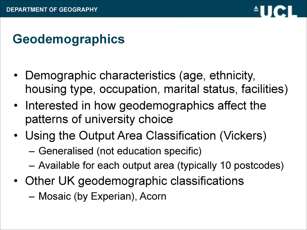
22. DEPARTMENT OF GEOGRAPHY A Good Model – Destination Simplifications • Attractiveness – Very subjective – different people like different things – Was originally modelled as a university “type” • Ancient, 19th century, Red brick, Plate glass, Post-1992 • Funding type: Big research-focused institution & hospital, 
 big research-focused, big teaching-based, small teaching – But difficult to categorise type and its relative effect on each of the origin geodemographics – Using Times Higher Education Score (range 200-1000) • Factor to modify its influence if necessary • Attractiveness becomes less important and location more important, as more of the flows become doubly constrained (i.e. more universities fill to capacity)
23. DEPARTMENT OF GEOGRAPHY Simplified Form • From: S ij = A i km e i km P i k (W j mh)αkm exp(-βkm c ij k) ! • To: S ij = A i k P i k (W j h)α exp(-βk d ij ) – No subject consideration – No “demand” factor – Cost is replaced by distance – Numbers of i, j locations greatly reduced – Attractiveness is not dependent on geodemographic • Similar for the doubly-constrained version
24. DEPARTMENT OF GEOGRAPHY Calibrating the Model • Find values for the constants in the equations • Ai & Bj values are “balancing constants” – they converge on the correct values during iteration • Calculate the βk distance-decay with known flows – Overall distance decay for all pupils – Break down by geodemographic • Very unequal numbers within each geodemographic – Compare distance decay functions
25. DEPARTMENT OF GEOGRAPHY Calibrating the Model – Beta Decay
26. DEPARTMENT OF GEOGRAPHY Calibrating the Model – Beta Decay • London to 
 Birmingham: 160 km • London to 
 Manchester: 260 km ! • Distinctive pattern seen for the City Living & Multicultural demographics
27. DEPARTMENT OF GEOGRAPHY Modelling • Java ! ! ! ! • Iterative process to calculate the normalising constants which depend on each other – Typically takes a minute to calculate the results
28. DEPARTMENT OF GEOGRAPHY Results • Simple Java GUI to show the matrix of results – visually spot good/poor matches – refine model parameters – rerun
29. DEPARTMENT OF GEOGRAPHY Results – Norfolk Schools to Universities
30. DEPARTMENT OF GEOGRAPHY Results – Schools to University of Manchester
31. DEPARTMENT OF GEOGRAPHY Results – Flow Maps • FlowMapLayout Java application – Developed at Stanford for InfoVis 2005 • A more graphic & flexible presentation of the flows – Pseudo-spatial – Lengths and directions of the connecting lines are not meaningful
32. DEPARTMENT OF GEOGRAPHY Results – Leeds Schools to Universities Predicted Actual
33. DEPARTMENT OF GEOGRAPHY Results – 
 Hampshire
 Schools to 
 Universities
34. DEPARTMENT OF GEOGRAPHY Some Interesting Anomalous Results • Flows significantly higher than expected – Flows from North-West London to Manchester – Essex to Exeter and Exeter to Essex – Small-distance flows to modern “metropolitan” universities, particularly paired with older institutions, such as Sheffield & Sheffield Hallam • Flows significantly lower than expected – Yorkshire to/from Lancashire – Essex to/from Kent
35. DEPARTMENT OF GEOGRAPHY Model Refinements • Creating a genuinely partially-constrained model – University capacities are not known, instead we assume the actual enrolled numbers are all at capacity – This results in a completely doubly-constrained model, unless the “not at university” option is made attractive. – Possible solution would be to increase all capacities by a small % and adjust “not at university” attractiveness to rebalance the numbers • The local “Metropolitan university” issue – Model adjusted to reduce the distances for these flows
36. DEPARTMENT OF GEOGRAPHY Further Considerations • Cost vs Distance – dij vs cij – Not necessarily linearly related for “life changing” spatial flows as such universities • Straight-line distance is too simple – Natural barriers (e.g. mountain ranges, water) – Fast intracity & intercity transport networks • Subject-specific analysis may be more revealing – e.g. flows for medicine courses only • Including Scottish/Wales data – Potentially interesting with different fee requirements
37. DEPARTMENT OF GEOGRAPHY References & Acknowledgements • Wilson, A.G. (2000). The widening access debate: student flows to universities and associated performance indicators. Environment and Planning A 32 pp 2019-31 • Phan D. Et al (2005). Flow Map Layout. http://graphics.stanford.edu/papers/ flow_map_layout/ • Dearden, J. and Wilson, A.G. (2008). An analysis system for exploring urban retail phase transitions – 1: an analysis system. CASA Working Papers Series 140 • Vickers, D.W. and Rees, P.H. (2007). Creating the National Statistics 2001 Output Area Classification. Journal of the Royal Statistical Society, Series A • The paper for this project is currently in review. ! Graphics Acknowledgements • Graphic for Newton's law of universal gravitation: Dennis Nilsson on Wikipedia • Homerton College of Technology: sarflondondunc on Flickr • Liverpool Street Station commuters: steve_way on Flickr • Aberystwyth University examination hall: jackhynes on Flickr • The maps use data from the OpenStreetMap project and contributors, and ONS boundary information
38. DEPARTMENT OF GEOGRAPHY Q&A ! ! ! ! Oliver O’Brien UCL Geography Twitter: @oobr http://www.oliverobrien.co.uk/ ESRC Funded Project