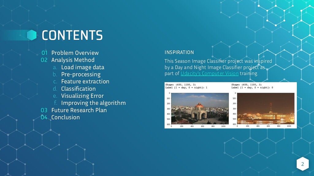
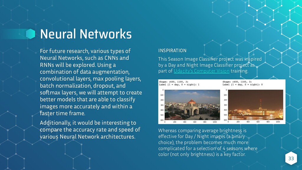
a Day and Night Image Classifier project as part of Udacity's Computer Vision training. 01 Problem Overview 02 Analysis Method a. Load image data b. Pre-processing c. Feature extraction d. Classification e. Visualizing Error f. Improving the algorithm 03 Future Research Plan 04 Conclusion 2
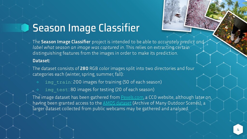
to be able to accurately predict and label what season an image was captured in. This relies on extracting certain distinguishing features from the images in order to make its prediction. Dataset: The dataset consists of 280 RGB color images split into two directories and four categories each (winter, spring, summer, fall): ⬥ img_train: 200 images for training (50 of each season) ⬥ img_test: 80 images for testing (20 of each season) The image dataset has been gathered from Pexels.com, a CC0 website, although later on, having been granted access to the AMOS dataset (Archive of Many Outdoor Scenes), a larger dataset collected from public webcams may be gathered and analyzed. 4
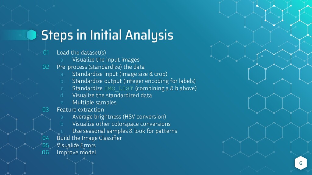
the input images 02 Pre-process (standardize) the data a. Standardize input (image size & crop) b. Standardize output (integer encoding for labels) c. Standardize IMG_LIST (combining a & b above) d. Visualize the standardized data e. Multiple samples 03 Feature extraction a. Average brightness (HSV conversion) b. Visualize other colorspace conversions c. Use seasonal samples & look for patterns 04 Build the Image Classifier 05 Visualize Errors 06 Improve model 6
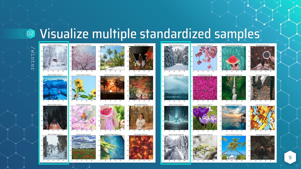
is pre-labeled so images can be automatically labeled appropriately: ⬥ /img ⬦ /train ⬩ /fall ⬩ /spring ⬩ /summer ⬩ /winter ⬦ /test ⬩ /fall ⬩ /spring ⬩ /summer ⬩ /winter 7 01 Data is loaded as it will be labeled: • 0: /winter • 1: /spring • 2: /summer • 3: /fall Each folder contains 50 images, so offsetting data by 50 changes the season we can visualize.
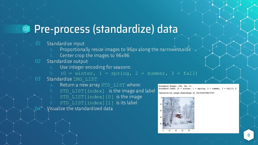
to 96px along the narrowest side b. Center crop the images to 96x96 02 Standardize output a. Use integer encoding for seasons: b. (0 = winter, 1 = spring, 2 = summer, 3 = fall) 03 Standardize IMG_LIST a. Return a new array STD_LIST where: b. STD_LIST[index] is the image and label c. STD_LIST[index][0] is the image d. STD_LIST[index][1] is its label 04 Visualize the standardized data 8 02
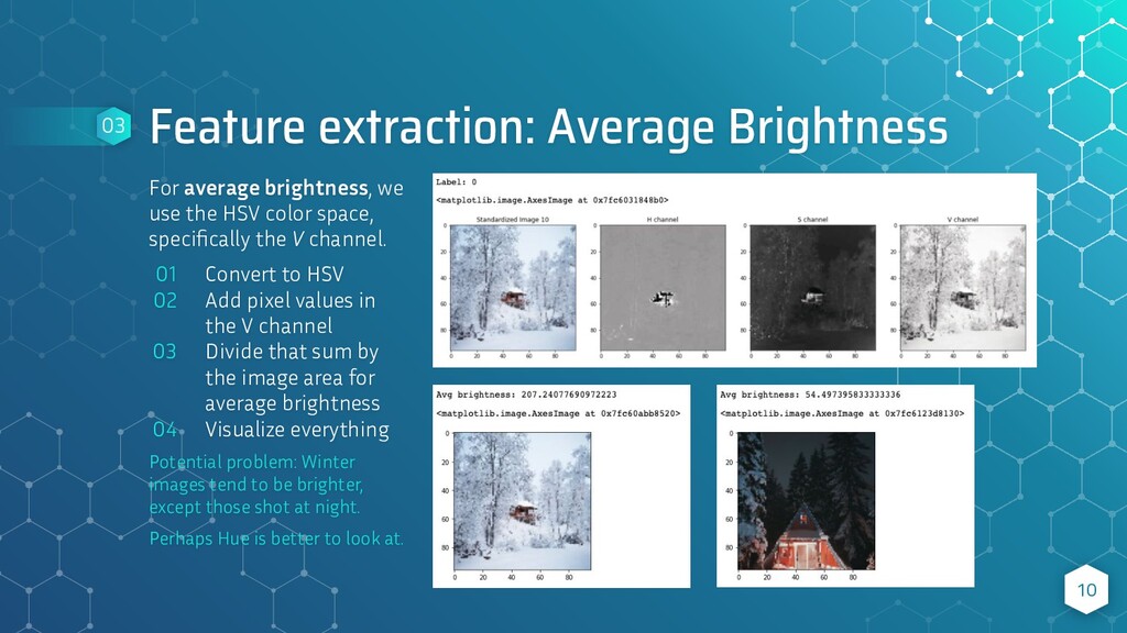
HSV color space, specifically the V channel. 01 Convert to HSV 02 Add pixel values in the V channel 03 Divide that sum by the image area for average brightness 04 Visualize everything Potential problem: Winter images tend to be brighter, except those shot at night. Perhaps Hue is better to look at. 10 03
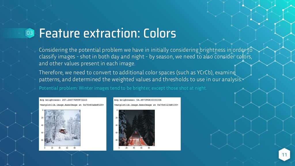
initially considering brightness in order to classify images - shot in both day and night - by season, we need to also consider colors, and other values present in each image. Therefore, we need to convert to additional color spaces (such as YCrCb), examine patterns, and determined the weighted values and thresholds to use in our analysis. Potential problem: Winter images tend to be brighter, except those shot at night. 11 03
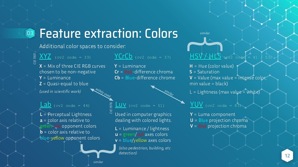
Mix of three CIE RGB curves chosen to be non-negative Y = Luminance Z = Quasi-equal to blue (used in scientific work) YCrCb (cv2 code = 37) Y = Luminance Cr = Red-difference chroma Cb = Blue-difference chrome HSV / HLS (cv2 code = 41 / 53) H = Hue (color value) S = Saturation V = Value (max value = intense color, min value = black) L = Lightness (max value = white) 12 Lab (cv2 code = 44) L = Perceptual Lightness a = color axis relative to green-red opponent colors b = color axis relative to blue-yellow opponent colors Luv (cv2 code = 51) Used in computer graphics dealing with colored lights. L = Luminance / lightness u = green/red axes colors v = blue/yellow axes colors (also pedestrian, building, etc detection) YUV (cv2 code = 83) Y = Luma component U = Blue projection chroma V = Red projection chroma 03 Additional color spaces to consider: similar } similar CIE 1931 CIE 1976 widely used } similar
same, Saturation, and Value / Lightness channels are reversed, but comparing them, nearly the same. Notes: HLS pulls more saturation from the day image. HSV pulls more saturation from the night image. Hue is light in both (winter) images. 13 03
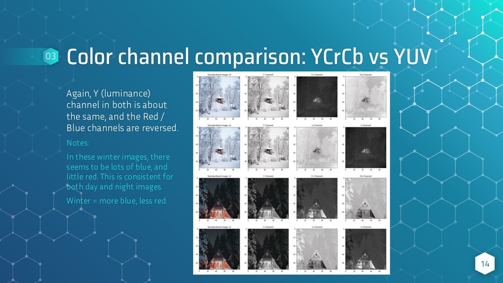
in both is about the same, and the Red / Blue channels are reversed. Notes: In these winter images, there seems to be lots of blue, and little red. This is consistent for both day and night images. Winter = more blue, less red. 14 03
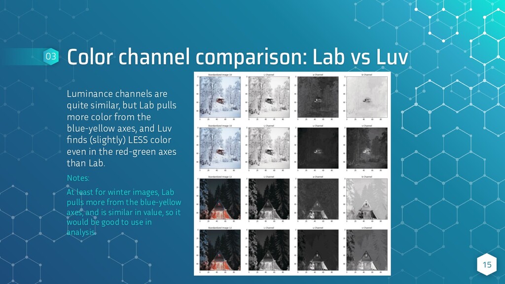
similar, but Lab pulls more color from the blue-yellow axes, and Luv finds (slightly) LESS color even in the red-green axes than Lab. Notes: At least for winter images, Lab pulls more from the blue-yellow axes, and is similar in value, so it would be good to use in analysis. 15 03
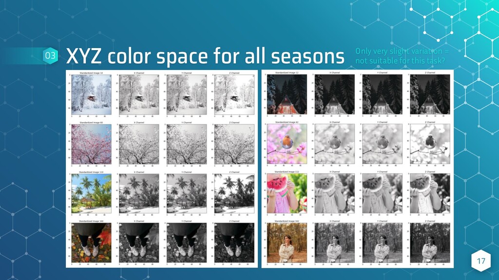
very similar across all channels for these (winter) images. Luv finds slightly more color in the blue-yellow axes, but less than Lab did previously. For the day image, it’s not really helpful. Notes: It would be interesting to compare XYZ colors for a sample from each season. 16 03
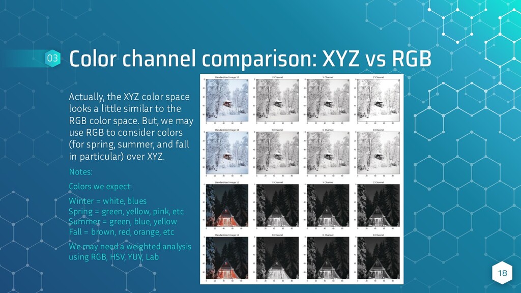
space looks a little similar to the RGB color space. But, we may use RGB to consider colors (for spring, summer, and fall in particular) over XYZ. Notes: Colors we expect: Winter = white, blues Spring = green, yellow, pink, etc Summer = green, blue, yellow Fall = brown, red, orange, etc We may need a weighted analysis using RGB, HSV, YUV, Lab 18 03
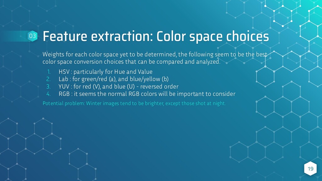
yet to be determined, the following seem to be the best color space conversion choices that can be compared and analyzed. 1. HSV : particularly for Hue and Value 2. Lab : for green/red (a), and blue/yellow (b) 3. YUV : for red (V), and blue (U) - reversed order 4. RGB : it seems the normal RGB colors will be important to consider Potential problem: Winter images tend to be brighter, except those shot at night. 19 03
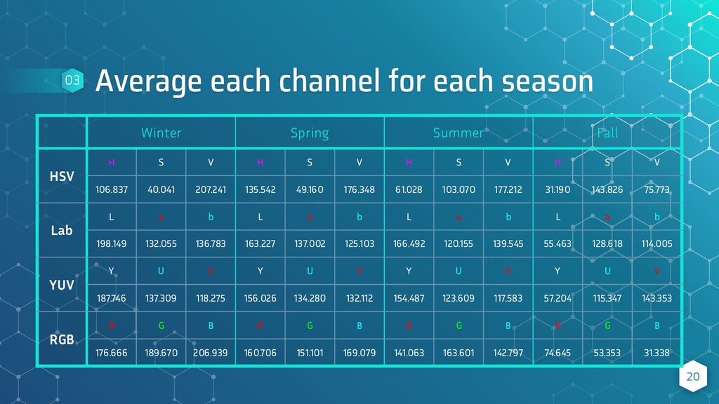
Summer Fall HSV H S V H S V H S V H S V 106.837 40.041 207.241 135.542 49.160 176.348 61.028 103.070 177.212 31.190 143.826 75.773 Lab L a b L a b L a b L a b 198.149 132.055 136.783 163.227 137.002 125.103 166.492 120.155 139.545 55.463 128.618 114.005 YUV Y U V Y U V Y U V Y U V 187.746 137.309 118.275 156.026 134.280 132.112 154.487 123.609 117.583 57.204 115.347 143.353 RGB R G B R G B R G B R G B 176.666 189.670 206.939 160.706 151.101 169.079 141.063 163.601 142.797 74.645 53.353 31.338
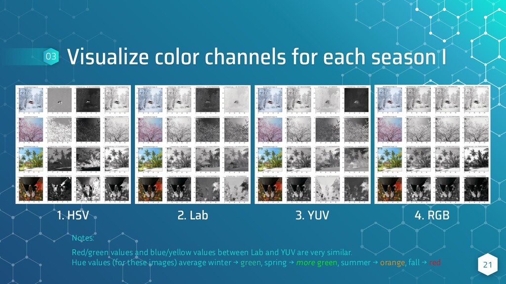
HSV 2. Lab 3. YUV 4. RGB Notes: Red/green values and blue/yellow values between Lab and YUV are very similar. Hue values (for these images) average winter → green, spring → more green, summer → orange, fall → red
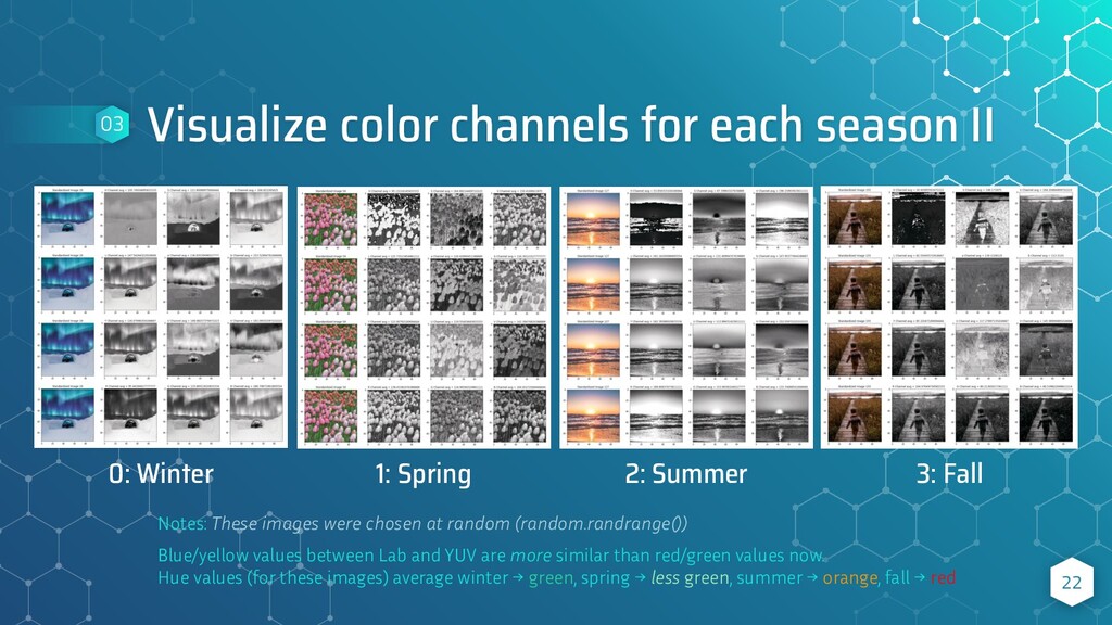
Winter 1: Spring 2: Summer 3: Fall Notes: These images were chosen at random (random.randrange()) Blue/yellow values between Lab and YUV are more similar than red/green values now. Hue values (for these images) average winter → green, spring → less green, summer → orange, fall → red
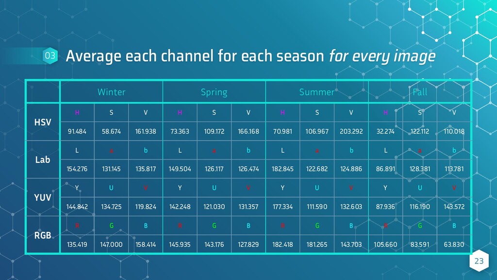
03 Winter Spring Summer Fall HSV H S V H S V H S V H S V 91.484 58.674 161.938 73.363 109.172 166.168 70.981 106.967 203.292 32.274 122.112 110.018 Lab L a b L a b L a b L a b 154.276 131.145 135.817 149.504 126.117 126.474 182.845 122.682 124.886 86.891 128.381 113.781 YUV Y U V Y U V Y U V Y U V 144.842 134.725 119.824 142.248 121.030 131.357 177.334 111.590 132.603 87.936 116.190 143.572 RGB R G B R G B R G B R G B 135.419 147.000 158.414 145.935 143.176 127.829 182.418 181.265 143.703 105.660 83.591 63.830
HSV H S V H S V H S V H S V Max 121.634 208.966 237.725 171.490 243.579 247.930 104.740 247.247 240.461 82.968 204.287 200.670 Avg 91.484 58.674 161.938 73.363 109.172 166.168 70.981 106.967 203.292 32.274 122.112 110.018 Min 0.0 0.0 51.614 16.365 27.326 97.968 13.892 49.113 84.479 10.864 40.033 53.595 stdev 63.342 107.779 93.588 78.466 109.186 75.083 45.921 101.885 81.474 37.030 82.127 74.198 Notes: Along with averages, I found max, min, and standard deviation between the three values Hues average winter → yellow-green, spring → less green, summer → yellow, fall → orange-red There is much less data variance in Summer and Fall’s Hue colors - those may be good indicators Fall’s brightness, and Winter’s saturation tend to be the lowest (although the value of 0.0 worries me)
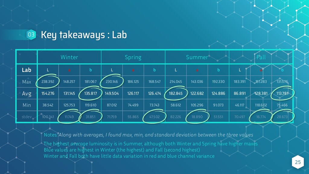
deviation between the three values The highest average luminosity is in Summer, although both Winter and Spring have higher maxes Blue values are highest in Winter (the highest) and Fall (second highest) Winter and Fall both have little data variation in red and blue channel variance Key takeaways : Lab 25 03 Winter Spring Summer Fall Lab L a b L a b L a b L a b Max 238.392 148.257 181.067 230.146 186.125 168.547 214.045 143.036 192.330 183.391 151.283 131.576 Avg 154.276 131.145 135.817 149.504 126.117 126.474 182.845 122.682 124.886 86.891 128.381 113.781 Min 38.542 125.753 119.610 87.012 74.499 73.743 58.612 105.296 91.073 46.117 118.602 75.466 stdev 100.341 11.749 31.851 71.759 55.865 47.502 82.226 18.890 51.551 70.497 16.774 28.673
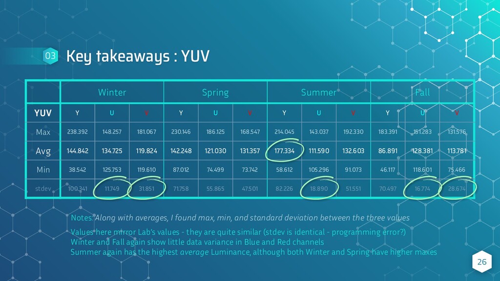
deviation between the three values Values here mirror Lab’s values - they are quite similar (stdev is identical - programming error?) Winter and Fall again show little data variance in Blue and Red channels Summer again has the highest average Luminance, although both Winter and Spring have higher maxes Key takeaways : YUV 26 03 Winter Spring Summer Fall YUV Y U V Y U V Y U V Y U V Max 238.392 148.257 181.067 230.146 186.125 168.547 214.045 143.037 192.330 183.391 151.283 131.576 Avg 144.842 134.725 119.824 142.248 121.030 131.357 177.334 111.590 132.603 86.891 128.381 113.781 Min 38.542 125.753 119.610 87.012 74.499 73.742 58.612 105.296 91.073 46.117 118.601 75.466 stdev 100.341 11.749 31.851 71.758 55.865 47.501 82.226 18.890 51.551 70.497 16.774 28.674
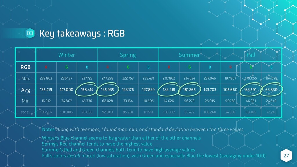
deviation between the three values Winter’s Blue channel seems to be greater than either of the other channels Spring’s Red channel tends to have the highest value Summer’s Red and Green channels both tend to have high average values Fall’s colors are all muted (low saturation), with Green and especially Blue the lowest (averaging under 100) Key takeaways : RGB 27 03 Winter Spring Summer Fall RGB R G B R G B R G B R G B Max 232.863 236.137 237.723 247.358 222.753 233.431 207.862 214.624 237.046 197.867 179.055 164.678 Avg 135.419 147.000 158.414 145.935 143.176 127.829 182.418 181.265 143.703 105.660 83.591 63.830 Min 16.212 34.807 45.336 62.028 33.164 10.505 14.026 56.273 25.015 50.782 46.261 24.649 stdev 108.507 100.885 96.686 92.803 95.201 111.514 105.337 83.477 106.268 74.328 68.485 72.242
◦ Lots of white ◦ More blue than other colors ◦ Brightly lit (except night) • Spring: ◦ Light greens ◦ Pinks, purples, yellows ◦ Brightly lit • Summer: ◦ Orange / red hue with sun ◦ Lots of greens (deeper) ◦ More blue • Fall: ◦ Muted colors ◦ Brown, dark green, orange ◦ Less brightly lit 28 03 Key characteristics (data): • Winter: ◦ HSV: Relatively low saturation (≈ 60, < 100) ◦ HSV: Average Hue = yellow-green (≈ 90) ◦ YUV: Low variance between B / R channels ◦ RGB: Slightly more blue than red • Spring: ◦ RGB: Red channel has a slightly higher value than either Blue or Green • Summer: ◦ HSV: Low data variance in Hue (≈ 70) ◦ Lab: Highest average luminosity (≈ 180) ◦ YUV: Low variance in Blue channel ◦ RGB: Red and Green values are high • Fall: ◦ HSV: Lowest brightness (≈ 100) ◦ HSV: Low variance in Hue = orange (≈ 30) ◦ YUV: Low variance in Blue / Red channels ◦ RGB: All color values are muted (near or < 100)
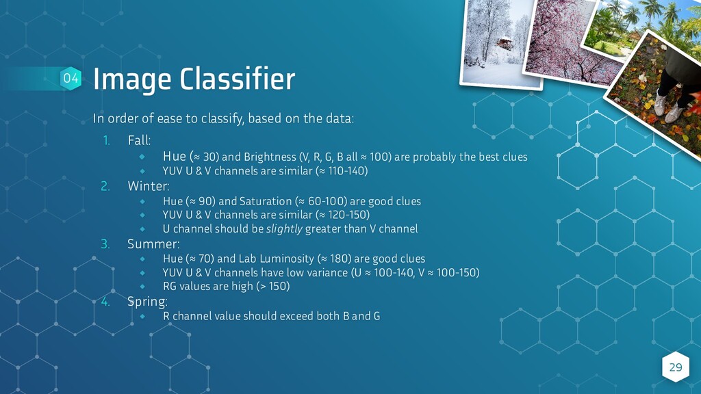
the data: 1. Fall: ⬦ Hue (≈ 30) and Brightness (V, R, G, B all ≈ 100) are probably the best clues ⬦ YUV U & V channels are similar (≈ 110-140) 2. Winter: ⬦ Hue (≈ 90) and Saturation (≈ 60-100) are good clues ⬦ YUV U & V channels are similar (≈ 120-150) ⬦ U channel should be slightly greater than V channel 3. Summer: ⬦ Hue (≈ 70) and Lab Luminosity (≈ 180) are good clues ⬦ YUV U & V channels have low variance (U ≈ 100-140, V ≈ 100-150) ⬦ RG values are high (> 150) 4. Spring: ⬦ R channel value should exceed both B and G 29 04
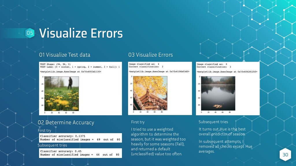
Accuracy First try Subsequent tries 03 Visualize Errors First try I tried to use a weighted algorithm to determine the season, but it was weighted too heavily for some seasons (Fall), and returned a default (unclassified) value too often. Subsequent tries It turns out Hue is the best overall predictor of season. In subsequent attempts, I removed all checks except Hue averages.
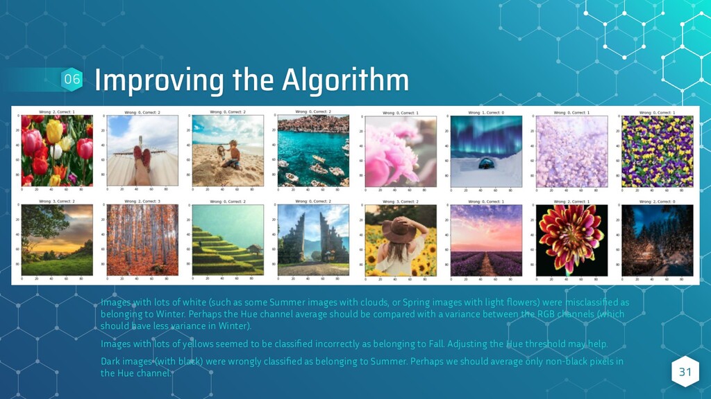
(such as some Summer images with clouds, or Spring images with light flowers) were misclassified as belonging to Winter. Perhaps the Hue channel average should be compared with a variance between the RGB channels (which should have less variance in Winter). Images with lots of yellows seemed to be classified incorrectly as belonging to Fall. Adjusting the Hue threshold may help. Dark images (with black) were wrongly classified as belonging to Summer. Perhaps we should average only non-black pixels in the Hue channel.
by a Day and Night Image Classifier project as part of Udacity's Computer Vision training. Whereas comparing average brightness is effective for Day / Night images (a binary choice), the problem becomes much more complicated for a selection of 4 seasons where color (not only brightness) is a key factor. For future research, various types of Neural Networks, such as CNNs and RNNs will be explored. Using a combination of data augmentation, convolutional layers, max pooling layers, batch normalization, dropout, and so max layers, we will attempt to create better models that are able to classify images more accurately and within a faster time frame. Additionally, it would be interesting to compare the accuracy rate and speed of various Neural Network architectures. 33
and pattern recognition on the part of a human programmer may be used to help develop an algorithm to classify images by season. However, there are various weaknesses inherent in this approach. Namely, that only color channels, such as Hue, Lightness, Red chroma, Blue chroma, and various combinations are used to classify images. This project does not take into account any sort of edge detection, or pixel gradient variation to help it classify images. Nor does it utilize a Neural Network for any kind of Machine Learning feature detection. (That’s for future research.) 35
code examples and output can be found at: https://github.com/jekkilekki/learning-opencv/blob/ main/computer-vision/Season%20Classifier.ipynb *Filesize may require download to view* 36