cs229-notes1.pdf

Transcript

1. CS229 Lecture notes Andrew Ng Supervised learning Lets start by talking about a few examples of supervised learning problems. Suppose we have a dataset giving the living areas and prices of 47 houses from Portland, Oregon: Living area (feet2) Price (1000$s) 2104 400 1600 330 2400 369 1416 232 3000 540 . . . . . . We can plot this data: 500 1000 1500 2000 2500 3000 3500 4000 4500 5000 0 100 200 300 400 500 600 700 800 900 1000 housing prices square feet price (in $1000) Given data like this, how can we learn to predict the prices of other houses in Portland, as a function of the size of their living areas? 1
2. CS229 Winter 2003 2 To establish notation for future use, we’ll use x(i) to denote the “input” variables (living area in this example), also called input features, and y(i) to denote the “output” or target variable that we are trying to predict (price). A pair (x(i), y(i)) is called a training example, and the dataset that we’ll be using to learn—a list of m training examples {(x(i), y(i)); i = 1, . . . , m}—is called a training set. Note that the superscript “(i)” in the notation is simply an index into the training set, and has nothing to do with exponentiation. We will also use X denote the space of input values, and Y the space of output values. In this example, X = Y = R. To describe the supervised learning problem slightly more formally, our goal is, given a training set, to learn a function h : X → Y so that h(x) is a “good” predictor for the corresponding value of y. For historical reasons, this function h is called a hypothesis. Seen pictorially, the process is therefore like this: Training set house.) (living area of Learning algorithm h predicted y x (predicted price) of house) When the target variable that we’re trying to predict is continuous, such as in our housing example, we call the learning problem a regression prob- lem. When y can take on only a small number of discrete values (such as if, given the living area, we wanted to predict if a dwelling is a house or an apartment, say), we call it a classification problem.
3. 3 Part I Linear Regression To make our housing example more interesting, lets consider a slightly richer dataset in which we also know the number of bedrooms in each house: Living area (feet2) #bedrooms Price (1000$s) 2104 3 400 1600 3 330 2400 3 369 1416 2 232 3000 4 540 . . . . . . . . . Here, the x’s are two-dimensional vectors in R2. For instance, x(i) 1 is the living area of the i-th house in the training set, and x(i) 2 is its number of bedrooms. (In general, when designing a learning problem, it will be up to you to decide what features to choose, so if you are out in Portland gathering housing data, you might also decide to include other features such as whether each house has a fireplace, the number of bathrooms, and so on. We’ll say more about feature selection later, but for now lets take the features as given.) To perform supervised learning, we must decide how we’re going to rep- resent functions/hypotheses h in a computer. As an initial choice, lets say we decide to approximate y as a linear function of x: hθ (x) = θ0 + θ1 x1 + θ2 x2 Here, the θi ’s are the parameters (also called weights) parameterizing the space of linear functions mapping from X to Y. When there is no risk of confusion, we will drop the θ subscript in hθ (x), and write it more simply as h(x). To simplify our notation, we also introduce the convention of letting x0 = 1 (this is the intercept term), so that h(x) = n i=0 θi xi = θT x, where on the right-hand side above we are viewing θ and x both as vectors, and here n is the number of input variables (not counting x0 ). Now, given a training set, how do we pick, or learn, the parameters θ? One reasonable method seems to be to make h(x) close to y, at least for
4. 4 the training examples we have. To formalize this, we will define a function that measures, for each value of the θ’s, how close the h(x(i))’s are to the corresponding y(i)’s. We define the cost function: J(θ) = 1 2 m i=1 (hθ (x(i)) − y(i))2. If you’ve seen linear regression before, you may recognize this as the familiar least-squares cost function that gives rise to the ordinary least squares regression model. Whether or not you have seen it previously, lets keep going, and we’ll eventually show this to be a special case of a much broader family of algorithms. 1 LMS algorithm We want to choose θ so as to minimize J(θ). To do so, lets use a search algorithm that starts with some “initial guess” for θ, and that repeatedly changes θ to make J(θ) smaller, until hopefully we converge to a value of θ that minimizes J(θ). Specifically, lets consider the gradient descent algorithm, which starts with some initial θ, and repeatedly performs the update: θj := θj − α ∂ ∂θj J(θ). (This update is simultaneously performed for all values of j = 0, . . . , n.) Here, α is called the learning rate. This is a very natural algorithm that repeatedly takes a step in the direction of steepest decrease of J. In order to implement this algorithm, we have to work out what is the partial derivative term on the right hand side. Lets first work it out for the case of if we have only one training example (x, y), so that we can neglect the sum in the definition of J. We have: ∂ ∂θj J(θ) = ∂ ∂θj 1 2 (hθ (x) − y)2 = 2 · 1 2 (hθ (x) − y) · ∂ ∂θj (hθ (x) − y) = (hθ (x) − y) · ∂ ∂θj n i=0 θi xi − y = (hθ (x) − y) xj
5. 5 For a single training example, this gives the update rule:1 θj := θj + α y(i) − hθ (x(i)) x(i) j . The rule is called the LMS update rule (LMS stands for “least mean squares”), and is also known as the Widrow-Hoff learning rule. This rule has several properties that seem natural and intuitive. For instance, the magnitude of the update is proportional to the error term (y(i) − hθ (x(i))); thus, for in- stance, if we are encountering a training example on which our prediction nearly matches the actual value of y(i), then we find that there is little need to change the parameters; in contrast, a larger change to the parameters will be made if our prediction hθ (x(i)) has a large error (i.e., if it is very far from y(i)). We’d derived the LMS rule for when there was only a single training example. There are two ways to modify this method for a training set of more than one example. The first is replace it with the following algorithm: Repeat until convergence { θj := θj + α m i=1 y(i) − hθ (x(i)) x(i) j (for every j). } The reader can easily verify that the quantity in the summation in the update rule above is just ∂J(θ)/∂θj (for the original definition of J). So, this is simply gradient descent on the original cost function J. This method looks at every example in the entire training set on every step, and is called batch gradient descent. Note that, while gradient descent can be susceptible to local minima in general, the optimization problem we have posed here for linear regression has only one global, and no other local, optima; thus gradient descent always converges (assuming the learning rate α is not too large) to the global minimum. Indeed, J is a convex quadratic function. Here is an example of gradient descent as it is run to minimize a quadratic function. 1We use the notation “a := b” to denote an operation (in a computer program) in which we set the value of a variable a to be equal to the value of b. In other words, this operation overwrites a with the value of b. In contrast, we will write “a = b” when we are asserting a statement of fact, that the value of a is equal to the value of b.
6. 6 5 10 15 20 25 30 35 40 45 50 5 10 15 20 25 30 35 40 45 50 The ellipses shown above are the contours of a quadratic function. Also shown is the trajectory taken by gradient descent, with was initialized at (48,30). The x’s in the figure (joined by straight lines) mark the successive values of θ that gradient descent went through. When we run batch gradient descent to fit θ on our previous dataset, to learn to predict housing price as a function of living area, we obtain θ0 = 71.27, θ1 = 0.1345. If we plot hθ (x) as a function of x (area), along with the training data, we obtain the following figure: 500 1000 1500 2000 2500 3000 3500 4000 4500 5000 0 100 200 300 400 500 600 700 800 900 1000 housing prices square feet price (in $1000) If the number of bedrooms were included as one of the input features as well, we get θ0 = 89.60, θ1 = 0.1392, θ2 = −8.738. The above results were obtained with batch gradient descent. There is an alternative to batch gradient descent that also works very well. Consider the following algorithm:
7. 7 Loop { for i=1 to m, { θj := θj + α y(i) − hθ (x(i)) x(i) j (for every j). } } In this algorithm, we repeatedly run through the training set, and each time we encounter a training example, we update the parameters according to the gradient of the error with respect to that single training example only. This algorithm is called stochastic gradient descent (also incremental gradient descent). Whereas batch gradient descent has to scan through the entire training set before taking a single step—a costly operation if m is large—stochastic gradient descent can start making progress right away, and continues to make progress with each example it looks at. Often, stochastic gradient descent gets θ “close” to the minimum much faster than batch gra- dient descent. (Note however that it may never “converge” to the minimum, and the parameters θ will keep oscillating around the minimum of J(θ); but in practice most of the values near the minimum will be reasonably good approximations to the true minimum.2) For these reasons, particularly when the training set is large, stochastic gradient descent is often preferred over batch gradient descent. 2 The normal equations Gradient descent gives one way of minimizing J. Lets discuss a second way of doing so, this time performing the minimization explicitly and without resorting to an iterative algorithm. In this method, we will minimize J by explicitly taking its derivatives with respect to the θj ’s, and setting them to zero. To enable us to do this without having to write reams of algebra and pages full of matrices of derivatives, lets introduce some notation for doing calculus with matrices. 2While it is more common to run stochastic gradient descent as we have described it and with a fixed learning rate α, by slowly letting the learning rate α decrease to zero as the algorithm runs, it is also possible to ensure that the parameters will converge to the global minimum rather then merely oscillate around the minimum.
8. 8 2.1 Matrix derivatives For a function f : Rm×n → R mapping from m-by-n matrices to the real numbers, we define the derivative of f with respect to A to be: ∇A f(A) =    ∂f ∂A11 · · · ∂f ∂A1n . . . ... . . . ∂f ∂Am1 · · · ∂f ∂Amn    Thus, the gradient ∇A f(A) is itself an m-by-n matrix, whose (i, j)-element is ∂f/∂Aij . For example, suppose A = A11 A12 A21 A22 is a 2-by-2 matrix, and the function f : R2×2 → R is given by f(A) = 3 2 A11 + 5A2 12 + A21 A22 . Here, Aij denotes the (i, j) entry of the matrix A. We then have ∇A f(A) = 3 2 10A12 A22 A21 . We also introduce the trace operator, written “tr.” For an n-by-n (square) matrix A, the trace of A is defined to be the sum of its diagonal entries: trA = n i=1 Aii If a is a real number (i.e., a 1-by-1 matrix), then tr a = a. (If you haven’t seen this “operator notation” before, you should think of the trace of A as tr(A), or as application of the “trace” function to the matrix A. It’s more commonly written without the parentheses, however.) The trace operator has the property that for two matrices A and B such that AB is square, we have that trAB = trBA. (Check this yourself!) As corollaries of this, we also have, e.g., trABC = trCAB = trBCA, trABCD = trDABC = trCDAB = trBCDA. The following properties of the trace operator are also easily verified. Here, A and B are square matrices, and a is a real number: trA = trAT tr(A + B) = trA + trB tr aA = atrA
9. 9 We now state without proof some facts of matrix derivatives (we won’t need some of these until later this quarter). Equation (4) applies only to non-singular square matrices A, where |A| denotes the determinant of A. We have: ∇A trAB = BT (1) ∇AT f(A) = (∇A f(A))T (2) ∇A trABAT C = CAB + CT ABT (3) ∇A |A| = |A|(A−1)T . (4) To make our matrix notation more concrete, let us now explain in detail the meaning of the first of these equations. Suppose we have some fixed matrix B ∈ Rn×m. We can then define a function f : Rm×n → R according to f(A) = trAB. Note that this definition makes sense, because if A ∈ Rm×n, then AB is a square matrix, and we can apply the trace operator to it; thus, f does indeed map from Rm×n to R. We can then apply our definition of matrix derivatives to find ∇A f(A), which will itself by an m-by-n matrix. Equation (1) above states that the (i, j) entry of this matrix will be given by the (i, j)-entry of BT , or equivalently, by Bji . The proofs of Equations (1-3) are reasonably simple, and are left as an exercise to the reader. Equations (4) can be derived using the adjoint repre- sentation of the inverse of a matrix.3 2.2 Least squares revisited Armed with the tools of matrix derivatives, let us now proceed to find in closed-form the value of θ that minimizes J(θ). We begin by re-writing J in matrix-vectorial notation. Giving a training set, define the design matrix X to be the m-by-n matrix (actually m-by-n + 1, if we include the intercept term) that contains 3If we define A′ to be the matrix whose (i, j) element is (−1)i+j times the determinant of the square matrix resulting from deleting row i and column j from A, then it can be proved that A−1 = (A′)T /|A|. (You can check that this is consistent with the standard way of finding A−1 when A is a 2-by-2 matrix. If you want to see a proof of this more general result, see an intermediate or advanced linear algebra text, such as Charles Curtis, 1991, Linear Algebra, Springer.) This shows that A′ = |A|(A−1)T . Also, the determinant of a matrix can be written |A| = j Aij A′ ij . Since (A′)ij does not depend on Aij (as can be seen from its definition), this implies that (∂/∂Aij )|A| = A′ ij . Putting all this together shows the result.
10. 10 the training examples’ input values in its rows: X =      — (x(1))T — — (x(2))T — . . . — (x(m))T —      . Also, let y be the m-dimensional vector containing all the target values from the training set: y =      y(1) y(2) . . . y(m)      . Now, since hθ (x(i)) = (x(i))T θ, we can easily verify that Xθ − y =    (x(1))T θ . . . (x(m))T θ    −    y(1) . . . y(m)    =    hθ (x(1)) − y(1) . . . hθ (x(m)) − y(m)    . Thus, using the fact that for a vector z, we have that zT z = i z2 i : 1 2 (Xθ − y)T (Xθ − y) = 1 2 m i=1 (hθ (x(i)) − y(i))2 = J(θ) Finally, to minimize J, lets find its derivatives with respect to θ. Combining Equations (2) and (3), we find that ∇AT trABAT C = BT AT CT + BAT C (5)
11. 11 Hence, ∇θ J(θ) = ∇θ 1 2 (Xθ − y)T (Xθ − y) = 1 2 ∇θ θT XT Xθ − θT XT y − yT Xθ + yT y = 1 2 ∇θ tr θT XT Xθ − θT XT y − yT Xθ + yT y = 1 2 ∇θ tr θT XT Xθ − 2tr yT Xθ = 1 2 XT Xθ + XT Xθ − 2XT y = XT Xθ − XT y In the third step, we used the fact that the trace of a real number is just the real number; the fourth step used the fact that trA = trAT , and the fifth step used Equation (5) with AT = θ, B = BT = XT X, and C = I, and Equation (1). To minimize J, we set its derivatives to zero, and obtain the normal equations: XT Xθ = XT y Thus, the value of θ that minimizes J(θ) is given in closed form by the equation θ = (XT X)−1XT y. 3 Probabilistic interpretation When faced with a regression problem, why might linear regression, and specifically why might the least-squares cost function J, be a reasonable choice? In this section, we will give a set of probabilistic assumptions, under which least-squares regression is derived as a very natural algorithm. Let us assume that the target variables and the inputs are related via the equation y(i) = θT x(i) + ǫ(i), where ǫ(i) is an error term that captures either unmodeled effects (such as if there are some features very pertinent to predicting housing price, but that we’d left out of the regression), or random noise. Let us further assume that the ǫ(i) are distributed IID (independently and identically distributed) according to a Gaussian distribution (also called a Normal distribution) with
12. 12 mean zero and some variance σ2. We can write this assumption as “ǫ(i) ∼ N(0, σ2).” I.e., the density of ǫ(i) is given by p(ǫ(i)) = 1 √ 2πσ exp − (ǫ(i))2 2σ2 . This implies that p(y(i)|x(i); θ) = 1 √ 2πσ exp − (y(i) − θT x(i))2 2σ2 . The notation “p(y(i)|x(i); θ)” indicates that this is the distribution of y(i) given x(i) and parameterized by θ. Note that we should not condition on θ (“p(y(i)|x(i), θ)”), since θ is not a random variable. We can also write the distribution of y(i) as as y(i) | x(i); θ ∼ N(θT x(i), σ2). Given X (the design matrix, which contains all the x(i)’s) and θ, what is the distribution of the y(i)’s? The probability of the data is given by p(y|X; θ). This quantity is typically viewed a function of y (and perhaps X), for a fixed value of θ. When we wish to explicitly view this as a function of θ, we will instead call it the likelihood function: L(θ) = L(θ; X, y) = p(y|X; θ). Note that by the independence assumption on the ǫ(i)’s (and hence also the y(i)’s given the x(i)’s), this can also be written L(θ) = m i=1 p(y(i) | x(i); θ) = m i=1 1 √ 2πσ exp − (y(i) − θT x(i))2 2σ2 . Now, given this probabilistic model relating the y(i)’s and the x(i)’s, what is a reasonable way of choosing our best guess of the parameters θ? The principal of maximum likelihood says that we should should choose θ so as to make the data as high probability as possible. I.e., we should choose θ to maximize L(θ). Instead of maximizing L(θ), we can also maximize any strictly increasing function of L(θ). In particular, the derivations will be a bit simpler if we
13. 13 instead maximize the log likelihood ℓ(θ): ℓ(θ) = log L(θ) = log m i=1 1 √ 2πσ exp − (y(i) − θT x(i))2 2σ2 = m i=1 log 1 √ 2πσ exp − (y(i) − θT x(i))2 2σ2 = m log 1 √ 2πσ − 1 σ2 · 1 2 m i=1 (y(i) − θT x(i))2. Hence, maximizing ℓ(θ) gives the same answer as minimizing 1 2 m i=1 (y(i) − θT x(i))2, which we recognize to be J(θ), our original least-squares cost function. To summarize: Under the previous probabilistic assumptions on the data, least-squares regression corresponds to finding the maximum likelihood esti- mate of θ. This is thus one set of assumptions under which least-squares re- gression can be justified as a very natural method that’s just doing maximum likelihood estimation. (Note however that the probabilistic assumptions are by no means necessary for least-squares to be a perfectly good and rational procedure, and there may—and indeed there are—other natural assumptions that can also be used to justify it.) Note also that, in our previous discussion, our final choice of θ did not depend on what was σ2, and indeed we’d have arrived at the same result even if σ2 were unknown. We will use this fact again later, when we talk about the exponential family and generalized linear models. 4 Locally weighted linear regression Consider the problem of predicting y from x ∈ R. The leftmost figure below shows the result of fitting a y = θ0 + θ1 x to a dataset. We see that the data doesn’t really lie on straight line, and so the fit is not very good.
14. 14 0 1 2 3 4 5 6 7 0 0.5 1 1.5 2 2.5 3 3.5 4 4.5 x y 0 1 2 3 4 5 6 7 0 0.5 1 1.5 2 2.5 3 3.5 4 4.5 x y 0 1 2 3 4 5 6 7 0 0.5 1 1.5 2 2.5 3 3.5 4 4.5 x y Instead, if we had added an extra feature x2, and fit y = θ0 + θ1 x + θ2 x2, then we obtain a slightly better fit to the data. (See middle figure) Naively, it might seem that the more features we add, the better. However, there is also a danger in adding too many features: The rightmost figure is the result of fitting a 5-th order polynomial y = 5 j=0 θj xj. We see that even though the fitted curve passes through the data perfectly, we would not expect this to be a very good predictor of, say, housing prices (y) for different living areas (x). Without formally defining what these terms mean, we’ll say the figure on the left shows an instance of underfitting—in which the data clearly shows structure not captured by the model—and the figure on the right is an example of overfitting. (Later in this class, when we talk about learning theory we’ll formalize some of these notions, and also define more carefully just what it means for a hypothesis to be good or bad.) As discussed previously, and as shown in the example above, the choice of features is important to ensuring good performance of a learning algorithm. (When we talk about model selection, we’ll also see algorithms for automat- ically choosing a good set of features.) In this section, let us talk briefly talk about the locally weighted linear regression (LWR) algorithm which, assum- ing there is sufficient training data, makes the choice of features less critical. This treatment will be brief, since you’ll get a chance to explore some of the properties of the LWR algorithm yourself in the homework. In the original linear regression algorithm, to make a prediction at a query point x (i.e., to evaluate h(x)), we would: 1. Fit θ to minimize i (y(i) − θT x(i))2. 2. Output θT x. In contrast, the locally weighted linear regression algorithm does the fol- lowing: 1. Fit θ to minimize i w(i)(y(i) − θT x(i))2. 2. Output θT x.
15. 15 Here, the w(i)’s are non-negative valued weights. Intuitively, if w(i) is large for a particular value of i, then in picking θ, we’ll try hard to make (y(i) − θT x(i))2 small. If w(i) is small, then the (y(i) − θT x(i))2 error term will be pretty much ignored in the fit. A fairly standard choice for the weights is4 w(i) = exp − (x(i) − x)2 2τ2 Note that the weights depend on the particular point x at which we’re trying to evaluate x. Moreover, if |x(i) − x| is small, then w(i) is close to 1; and if |x(i) − x| is large, then w(i) is small. Hence, θ is chosen giving a much higher “weight” to the (errors on) training examples close to the query point x. (Note also that while the formula for the weights takes a form that is cosmetically similar to the density of a Gaussian distribution, the w(i)’s do not directly have anything to do with Gaussians, and in particular the w(i) are not random variables, normally distributed or otherwise.) The parameter τ controls how quickly the weight of a training example falls off with distance of its x(i) from the query point x; τ is called the bandwidth parameter, and is also something that you’ll get to experiment with in your homework. Locally weighted linear regression is the first example we’re seeing of a non-parametric algorithm. The (unweighted) linear regression algorithm that we saw earlier is known as a parametric learning algorithm, because it has a fixed, finite number of parameters (the θi ’s), which are fit to the data. Once we’ve fit the θi ’s and stored them away, we no longer need to keep the training data around to make future predictions. In contrast, to make predictions using locally weighted linear regression, we need to keep the entire training set around. The term “non-parametric” (roughly) refers to the fact that the amount of stuff we need to keep in order to represent the hypothesis h grows linearly with the size of the training set. 4If x is vector-valued, this is generalized to be w(i) = exp(−(x(i) −x)T (x(i) −x)/(2τ2)), or w(i) = exp(−(x(i) − x)T Σ−1(x(i) − x)/2), for an appropriate choice of τ or Σ.
16. 16 Part II Classification and logistic regression Lets now talk about the classification problem. This is just like the regression problem, except that the values y we now want to predict take on only a small number of discrete values. For now, we will focus on the binary classification problem in which y can take on only two values, 0 and 1. (Most of what we say here will also generalize to the multiple-class case.) For instance, if we are trying to build a spam classifier for email, then x(i) may be some features of a piece of email, and y may be 1 if it is a piece of spam mail, and 0 otherwise. 0 is also called the negative class, and 1 the positive class, and they are sometimes also denoted by the symbols “-” and “+.” Given x(i), the corresponding y(i) is also called the label for the training example. 5 Logistic regression We could approach the classification problem ignoring the fact that y is discrete-valued, and use our old linear regression algorithm to try to predict y given x. However, it is easy to construct examples where this method performs very poorly. Intuitively, it also doesn’t make sense for hθ (x) to take values larger than 1 or smaller than 0 when we know that y ∈ {0, 1}. To fix this, lets change the form for our hypotheses hθ (x). We will choose hθ (x) = g(θT x) = 1 1 + e−θT x , where g(z) = 1 1 + e−z is called the logistic function or the sigmoid function. Here is a plot showing g(z):
17. 17 −5 −4 −3 −2 −1 0 1 2 3 4 5 0 0.1 0.2 0.3 0.4 0.5 0.6 0.7 0.8 0.9 1 z g(z) Notice that g(z) tends towards 1 as z → ∞, and g(z) tends towards 0 as z → −∞. Moreover, g(z), and hence also h(x), is always bounded between 0 and 1. As before, we are keeping the convention of letting x0 = 1, so that θT x = θ0 + n j=1 θj xj . For now, lets take the choice of g as given. Other functions that smoothly increase from 0 to 1 can also be used, but for a couple of reasons that we’ll see later (when we talk about GLMs, and when we talk about generative learning algorithms), the choice of the logistic function is a fairly natural one. Before moving on, here’s a useful property of the derivative of the sigmoid function, which we write a g′: g′(z) = d dz 1 1 + e−z = 1 (1 + e−z)2 e−z = 1 (1 + e−z) · 1 − 1 (1 + e−z) = g(z)(1 − g(z)). So, given the logistic regression model, how do we fit θ for it? Follow- ing how we saw least squares regression could be derived as the maximum likelihood estimator under a set of assumptions, lets endow our classification model with a set of probabilistic assumptions, and then fit the parameters via maximum likelihood.
18. 18 Let us assume that P(y = 1 | x; θ) = hθ (x) P(y = 0 | x; θ) = 1 − hθ (x) Note that this can be written more compactly as p(y | x; θ) = (hθ (x))y (1 − hθ (x))1−y Assuming that the m training examples were generated independently, we can then write down the likelihood of the parameters as L(θ) = p(y | X; θ) = m i=1 p(y(i) | x(i); θ) = m i=1 hθ (x(i)) y(i) 1 − hθ (x(i)) 1−y(i) As before, it will be easier to maximize the log likelihood: ℓ(θ) = log L(θ) = m i=1 y(i) log h(x(i)) + (1 − y(i)) log(1 − h(x(i))) How do we maximize the likelihood? Similar to our derivation in the case of linear regression, we can use gradient ascent. Written in vectorial notation, our updates will therefore be given by θ := θ + α∇θ ℓ(θ). (Note the positive rather than negative sign in the update formula, since we’re maximizing, rather than minimizing, a function now.) Lets start by working with just one training example (x, y), and take derivatives to derive the stochastic gradient ascent rule: ∂ ∂θj ℓ(θ) = y 1 g(θT x) − (1 − y) 1 1 − g(θT x) ∂ ∂θj g(θT x) = y 1 g(θT x) − (1 − y) 1 1 − g(θT x) g(θT x)(1 − g(θT x) ∂ ∂θj θT x = y(1 − g(θT x)) − (1 − y)g(θT x) xj = (y − hθ (x)) xj
19. 19 Above, we used the fact that g′(z) = g(z)(1 − g(z)). This therefore gives us the stochastic gradient ascent rule θj := θj + α y(i) − hθ (x(i)) x(i) j If we compare this to the LMS update rule, we see that it looks identical; but this is not the same algorithm, because hθ (x(i)) is now defined as a non-linear function of θT x(i). Nonetheless, it’s a little surprising that we end up with the same update rule for a rather different algorithm and learning problem. Is this coincidence, or is there a deeper reason behind this? We’ll answer this when get get to GLM models. (See also the extra credit problem on Q3 of problem set 1.) 6 Digression: The perceptron learning algo- rithm We now digress to talk briefly about an algorithm that’s of some historical interest, and that we will also return to later when we talk about learning theory. Consider modifying the logistic regression method to “force” it to output values that are either 0 or 1 or exactly. To do so, it seems natural to change the definition of g to be the threshold function: g(z) = 1 if z ≥ 0 0 if z < 0 If we then let hθ (x) = g(θT x) as before but using this modified definition of g, and if we use the update rule θj := θj + α y(i) − hθ (x(i)) x(i) j . then we have the perceptron learning algorithm. In the 1960s, this “perceptron” was argued to be a rough model for how individual neurons in the brain work. Given how simple the algorithm is, it will also provide a starting point for our analysis when we talk about learning theory later in this class. Note however that even though the perceptron may be cosmetically similar to the other algorithms we talked about, it is actually a very different type of algorithm than logistic regression and least squares linear regression; in particular, it is difficult to endow the perceptron’s predic- tions with meaningful probabilistic interpretations, or derive the perceptron as a maximum likelihood estimation algorithm.
20. 20 7 Another algorithm for maximizing ℓ(θ) Returning to logistic regression with g(z) being the sigmoid function, lets now talk about a different algorithm for minimizing ℓ(θ). To get us started, lets consider Newton’s method for finding a zero of a function. Specifically, suppose we have some function f : R → R, and we wish to find a value of θ so that f(θ) = 0. Here, θ ∈ R is a real number. Newton’s method performs the following update: θ := θ − f(θ) f′(θ) . This method has a natural interpretation in which we can think of it as approximating the function f via a linear function that is tangent to f at the current guess θ, solving for where that linear function equals to zero, and letting the next guess for θ be where that linear function is zero. Here’s a picture of the Newton’s method in action: 1 1.5 2 2.5 3 3.5 4 4.5 5 −10 0 10 20 30 40 50 60 x f(x) 1 1.5 2 2.5 3 3.5 4 4.5 5 −10 0 10 20 30 40 50 60 x f(x) 1 1.5 2 2.5 3 3.5 4 4.5 5 −10 0 10 20 30 40 50 60 x f(x) In the leftmost figure, we see the function f plotted along with the line y = 0. We’re trying to find θ so that f(θ) = 0; the value of θ that achieves this is about 1.3. Suppose we initialized the algorithm with θ = 4.5. Newton’s method then fits a straight line tangent to f at θ = 4.5, and solves for the where that line evaluates to 0. (Middle figure.) This give us the next guess for θ, which is about 2.8. The rightmost figure shows the result of running one more iteration, which the updates θ to about 1.8. After a few more iterations, we rapidly approach θ = 1.3. Newton’s method gives a way of getting to f(θ) = 0. What if we want to use it to maximize some function ℓ? The maxima of ℓ correspond to points where its first derivative ℓ′(θ) is zero. So, by letting f(θ) = ℓ′(θ), we can use the same algorithm to maximize ℓ, and we obtain update rule: θ := θ − ℓ′(θ) ℓ′′(θ) . (Something to think about: How would this change if we wanted to use Newton’s method to minimize rather than maximize a function?)
21. 21 Lastly, in our logistic regression setting, θ is vector-valued, so we need to generalize Newton’s method to this setting. The generalization of Newton’s method to this multidimensional setting (also called the Newton-Raphson method) is given by θ := θ − H−1∇θ ℓ(θ). Here, ∇θ ℓ(θ) is, as usual, the vector of partial derivatives of ℓ(θ) with respect to the θi ’s; and H is an n-by-n matrix (actually, n + 1-by-n + 1, assuming that we include the intercept term) called the Hessian, whose entries are given by Hij = ∂2ℓ(θ) ∂θi ∂θj . Newton’s method typically enjoys faster convergence than (batch) gra- dient descent, and requires many fewer iterations to get very close to the minimum. One iteration of Newton’s can, however, be more expensive than one iteration of gradient descent, since it requires finding and inverting an n-by-n Hessian; but so long as n is not too large, it is usually much faster overall. When Newton’s method is applied to maximize the logistic regres- sion log likelihood function ℓ(θ), the resulting method is also called Fisher scoring.
22. 22 Part III Generalized Linear Models5 So far, we’ve seen a regression example, and a classification example. In the regression example, we had y|x; θ ∼ N(µ, σ2), and in the classification one, y|x; θ ∼ Bernoulli(φ), where for some appropriate definitions of µ and φ as functions of x and θ. In this section, we will show that both of these methods are special cases of a broader family of models, called Generalized Linear Models (GLMs). We will also show how other models in the GLM family can be derived and applied to other classification and regression problems. 8 The exponential family To work our way up to GLMs, we will begin by defining exponential family distributions. We say that a class of distributions is in the exponential family if it can be written in the form p(y; η) = b(y) exp(ηT T(y) − a(η)) (6) Here, η is called the natural parameter (also called the canonical param- eter) of the distribution; T(y) is the sufficient statistic (for the distribu- tions we consider, it will often be the case that T(y) = y); and a(η) is the log partition function. The quantity e−a(η) essentially plays the role of a nor- malization constant, that makes sure the distribution p(y; η) sums/integrates over y to 1. A fixed choice of T, a and b defines a family (or set) of distributions that is parameterized by η; as we vary η, we then get different distributions within this family. We now show that the Bernoulli and the Gaussian distributions are ex- amples of exponential family distributions. The Bernoulli distribution with mean φ, written Bernoulli(φ), specifies a distribution over y ∈ {0, 1}, so that p(y = 1; φ) = φ; p(y = 0; φ) = 1 − φ. As we varying φ, we obtain Bernoulli distributions with different means. We now show that this class of Bernoulli distributions, ones obtained by varying φ, is in the exponential family; i.e., that there is a choice of T, a and b so that Equation (6) becomes exactly the class of Bernoulli distributions. 5The presentation of the material in this section takes inspiration from Michael I. Jordan, Learning in graphical models (unpublished book draft), and also McCullagh and Nelder, Generalized Linear Models (2nd ed.).
23. 23 We write the Bernoulli distribution as: p(y; φ) = φy(1 − φ)1−y = exp(y log φ + (1 − y) log(1 − φ)) = exp log φ 1 − φ y + log(1 − φ) . Thus, the natural parameter is given by η = log(φ/(1 − φ)). Interestingly, if we invert this definition for η by solving for φ in terms of η, we obtain φ = 1/(1 + e−η). This is the familiar sigmoid function! This will come up again when we derive logistic regression as a GLM. To complete the formulation of the Bernoulli distribution as an exponential family distribution, we also have T(y) = y a(η) = − log(1 − φ) = log(1 + eη) b(y) = 1 This shows that the Bernoulli distribution can be written in the form of Equation (6), using an appropriate choice of T, a and b. Lets now move on to consider the Gaussian distribution. Recall that, when deriving linear regression, the value of σ2 had no effect on our final choice of θ and hθ (x). Thus, we can choose an arbitrary value for σ2 without changing anything. To simplify the derivation below, lets set σ2 = 1.6 We then have: p(y; µ) = 1 √ 2π exp − 1 2 (y − µ)2 = 1 √ 2π exp − 1 2 y2 · exp µy − 1 2 µ2 6If we leave σ2 as a variable, the Gaussian distribution can also be shown to be in the exponential family, where η ∈ R2 is now a 2-dimension vector that depends on both µ and σ. For the purposes of GLMs, however, the σ2 parameter can also be treated by considering a more general definition of the exponential family: p(y; η, τ) = b(a, τ) exp((ηT T(y) − a(η))/c(τ)). Here, τ is called the dispersion parameter, and for the Gaussian, c(τ) = σ2; but given our simplification above, we won’t need the more general definition for the examples we will consider here.
24. 24 Thus, we see that the Gaussian is in the exponential family, with η = µ T(y) = y a(η) = µ2/2 = η2/2 b(y) = (1/ √ 2π) exp(−y2/2). There’re many other distributions that are members of the exponen- tial family: The multinomial (which we’ll see later), the Poisson (for mod- elling count-data; also see the problem set); the gamma and the exponen- tial (for modelling continuous, non-negative random variables, such as time- intervals); the beta and the Dirichlet (for distributions over probabilities); and many more. In the next section, we will describe a general “recipe” for constructing models in which y (given x and θ) comes from any of these distributions. 9 Constructing GLMs Suppose you would like to build a model to estimate the number y of cus- tomers arriving in your store (or number of page-views on your website) in any given hour, based on certain features x such as store promotions, recent advertising, weather, day-of-week, etc. We know that the Poisson distribu- tion usually gives a good model for numbers of visitors. Knowing this, how can we come up with a model for our problem? Fortunately, the Poisson is an exponential family distribution, so we can apply a Generalized Linear Model (GLM). In this section, we will we will describe a method for constructing GLM models for problems such as these. More generally, consider a classification or regression problem where we would like to predict the value of some random variable y as a function of x. To derive a GLM for this problem, we will make the following three assumptions about the conditional distribution of y given x and about our model: 1. y | x; θ ∼ ExponentialFamily(η). I.e., given x and θ, the distribution of y follows some exponential family distribution, with parameter η. 2. Given x, our goal is to predict the expected value of T(y) given x. In most of our examples, we will have T(y) = y, so this means we would like the prediction h(x) output by our learned hypothesis h to
25. 25 satisfy h(x) = E[y|x]. (Note that this assumption is satisfied in the choices for hθ (x) for both logistic regression and linear regression. For instance, in logistic regression, we had hθ (x) = p(y = 1|x; θ) = 0 · p(y = 0|x; θ) + 1 · p(y = 1|x; θ) = E[y|x; θ].) 3. The natural parameter η and the inputs x are related linearly: η = θT x. (Or, if η is vector-valued, then ηi = θT i x.) The third of these assumptions might seem the least well justified of the above, and it might be better thought of as a “design choice” in our recipe for designing GLMs, rather than as an assumption per se. These three assumptions/design choices will allow us to derive a very elegant class of learning algorithms, namely GLMs, that have many desirable properties such as ease of learning. Furthermore, the resulting models are often very effective for modelling different types of distributions over y; for example, we will shortly show that both logistic regression and ordinary least squares can both be derived as GLMs. 9.1 Ordinary Least Squares To show that ordinary least squares is a special case of the GLM family of models, consider the setting where the target variable y (also called the response variable in GLM terminology) is continuous, and we model the conditional distribution of y given x as as a Gaussian N(µ, σ2). (Here, µ may depend x.) So, we let the ExponentialFamily(η) distribution above be the Gaussian distribution. As we saw previously, in the formulation of the Gaussian as an exponential family distribution, we had µ = η. So, we have hθ (x) = E[y|x; θ] = µ = η = θT x. The first equality follows from Assumption 2, above; the second equality follows from the fact that y|x; θ ∼ N(µ, σ2), and so its expected value is given by µ; the third equality follows from Assumption 1 (and our earlier derivation showing that µ = η in the formulation of the Gaussian as an exponential family distribution); and the last equality follows from Assumption 3.
26. 26 9.2 Logistic Regression We now consider logistic regression. Here we are interested in binary classifi- cation, so y ∈ {0, 1}. Given that y is binary-valued, it therefore seems natural to choose the Bernoulli family of distributions to model the conditional dis- tribution of y given x. In our formulation of the Bernoulli distribution as an exponential family distribution, we had φ = 1/(1 + e−η). Furthermore, note that if y|x; θ ∼ Bernoulli(φ), then E[y|x; θ] = φ. So, following a similar derivation as the one for ordinary least squares, we get: hθ (x) = E[y|x; θ] = φ = 1/(1 + e−η) = 1/(1 + e−θT x) So, this gives us hypothesis functions of the form hθ (x) = 1/(1 + e−θT x). If you are previously wondering how we came up with the form of the logistic function 1/(1 + e−z), this gives one answer: Once we assume that y condi- tioned on x is Bernoulli, it arises as a consequence of the definition of GLMs and exponential family distributions. To introduce a little more terminology, the function g giving the distri- bution’s mean as a function of the natural parameter (g(η) = E[T(y); η]) is called the canonical response function. Its inverse, g−1, is called the canonical link function. Thus, the canonical response function for the Gaussian family is just the identify function; and the canonical response function for the Bernoulli is the logistic function.7 9.3 Softmax Regression Lets look at one more example of a GLM. Consider a classification problem in which the response variable y can take on any one of k values, so y ∈ {1 2, . . . , k}. For example, rather than classifying email into the two classes spam or not-spam—which would have been a binary classification problem— we might want to classify it into three classes, such as spam, personal mail, and work-related mail. The response variable is still discrete, but can now take on more than two values. We will thus model it as distributed according to a multinomial distribution. 7Many texts use g to denote the link function, and g−1 to denote the response function; but the notation we’re using here, inherited from the early machine learning literature, will be more consistent with the notation used in the rest of the class.
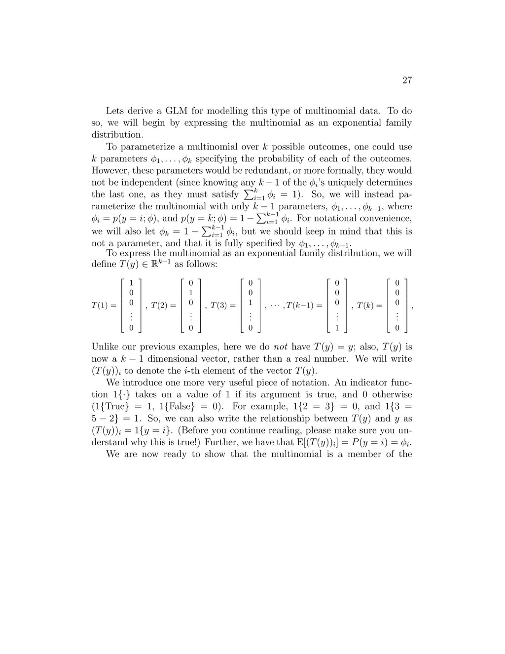
27. 27 Lets derive a GLM for modelling this type of multinomial data. To do so, we will begin by expressing the multinomial as an exponential family distribution. To parameterize a multinomial over k possible outcomes, one could use k parameters φ1 , . . . , φk specifying the probability of each of the outcomes. However, these parameters would be redundant, or more formally, they would not be independent (since knowing any k − 1 of the φi ’s uniquely determines the last one, as they must satisfy k i=1 φi = 1). So, we will instead pa- rameterize the multinomial with only k − 1 parameters, φ1 , . . . , φk−1 , where φi = p(y = i; φ), and p(y = k; φ) = 1 − k−1 i=1 φi . For notational convenience, we will also let φk = 1 − k−1 i=1 φi , but we should keep in mind that this is not a parameter, and that it is fully specified by φ1 , . . . , φk−1 . To express the multinomial as an exponential family distribution, we will define T(y) ∈ Rk−1 as follows: T(1) =        1 0 0 . . . 0        , T(2) =        0 1 0 . . . 0        , T(3) =        0 0 1 . . . 0        , · · · , T(k−1) =        0 0 0 . . . 1        , T(k) =        0 0 0 . . . 0        , Unlike our previous examples, here we do not have T(y) = y; also, T(y) is now a k − 1 dimensional vector, rather than a real number. We will write (T(y))i to denote the i-th element of the vector T(y). We introduce one more very useful piece of notation. An indicator func- tion 1{·} takes on a value of 1 if its argument is true, and 0 otherwise (1{True} = 1, 1{False} = 0). For example, 1{2 = 3} = 0, and 1{3 = 5 − 2} = 1. So, we can also write the relationship between T(y) and y as (T(y))i = 1{y = i}. (Before you continue reading, please make sure you un- derstand why this is true!) Further, we have that E[(T(y))i ] = P(y = i) = φi . We are now ready to show that the multinomial is a member of the
28. 28 exponential family. We have: p(y; φ) = φ1{y=1} 1 φ1{y=2} 2 · · · φ1{y=k} k = φ1{y=1} 1 φ1{y=2} 2 · · · φ1−Pk−1 i=1 1{y=i} k = φ(T(y))1 1 φ(T(y))2 2 · · · φ1−Pk−1 i=1 (T(y))i k = exp((T(y))1 log(φ1 ) + (T(y))2 log(φ2 ) + · · · + 1 − k−1 i=1 (T(y))i log(φk )) = exp((T(y))1 log(φ1 /φk ) + (T(y))2 log(φ2 /φk ) + · · · + (T(y))k−1 log(φk−1 /φk ) + log(φk )) = b(y) exp(ηT T(y) − a(η)) where η =      log(φ1 /φk ) log(φ2 /φk ) . . . log(φk−1 /φk )      , a(η) = − log(φk ) b(y) = 1. This completes our formulation of the multinomial as an exponential family distribution. The link function is given (for i = 1, . . . , k) by ηi = log φi φk . For convenience, we have also defined ηk = log(φk /φk ) = 0. To invert the link function and derive the response function, we therefore have that eηi = φi φk φk eηi = φi (7) φk k i=1 eηi = k i=1 φi = 1 This implies that φk = 1/ k i=1 eηi , which can be substituted back into Equa- tion (7) to give the response function φi = eηi k j=1 eηj
29. 29 This function mapping from the η’s to the φ’s is called the softmax function. To complete our model, we use Assumption 3, given earlier, that the ηi ’s are linearly related to the x’s. So, have ηi = θT i x (for i = 1, . . . , k − 1), where θ1 , . . . , θk−1 ∈ Rn+1 are the parameters of our model. For notational convenience, we can also define θk = 0, so that ηk = θT k x = 0, as given previously. Hence, our model assumes that the conditional distribution of y given x is given by p(y = i|x; θ) = φi = eηi k j=1 eηj = eθT i x k j=1 eθT j x (8) This model, which applies to classification problems where y ∈ {1, . . . , k}, is called softmax regression. It is a generalization of logistic regression. Our hypothesis will output hθ (x) = E[T(y)|x; θ] = E      1{y = 1} 1{y = 2} . . . 1{y = k − 1} x; θ      =      φ1 φ2 . . . φk−1      =         exp(θT 1 x) Pk j=1 exp(θT j x) exp(θT 2 x) Pk j=1 exp(θT j x) . . . exp(θT k−1 x) Pk j=1 exp(θT j x)         . In other words, our hypothesis will output the estimated probability that p(y = i|x; θ), for every value of i = 1, . . . , k. (Even though hθ (x) as defined above is only k − 1 dimensional, clearly p(y = k|x; θ) can be obtained as 1 − k−1 i=1 φi .)
30. 30 Lastly, lets discuss parameter fitting. Similar to our original derivation of ordinary least squares and logistic regression, if we have a training set of m examples {(x(i), y(i)); i = 1, . . . , m} and would like to learn the parameters θi of this model, we would begin by writing down the log-likelihood ℓ(θ) = m i=1 log p(y(i)|x(i); θ) = m i=1 log k l=1 eθT l x(i) k j=1 eθT j x(i) 1{y(i)=l} To obtain the second line above, we used the definition for p(y|x; θ) given in Equation (8). We can now obtain the maximum likelihood estimate of the parameters by maximizing ℓ(θ) in terms of θ, using a method such as gradient ascent or Newton’s method.