Comparing Variation with granovagg.1w

The addition of stacked variance bars

Transcript

1. Next-­‐Generation  granova A ggplot2 package for graphical Analysis of Variance Brian Danielak briandk@umd.edu 1
2. https://www.github.com/briandk/granova 2
3. 3 granova.1w() granova.2w() granova.contr() granova.ds()
4. In the previous version, stacks were proportional in height to a group’s standard deviation. Comparing Variation 4 • −0.067 −0.16 −0.14 0.088 −0.1 0.13 0.19 −0.15 0
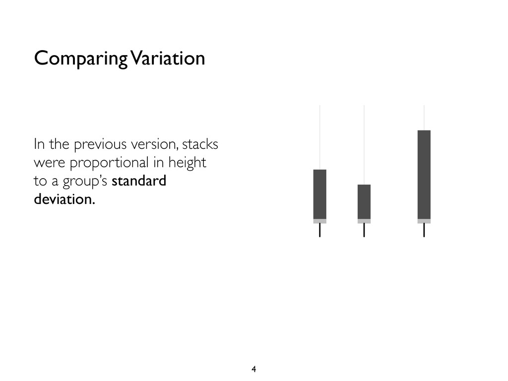
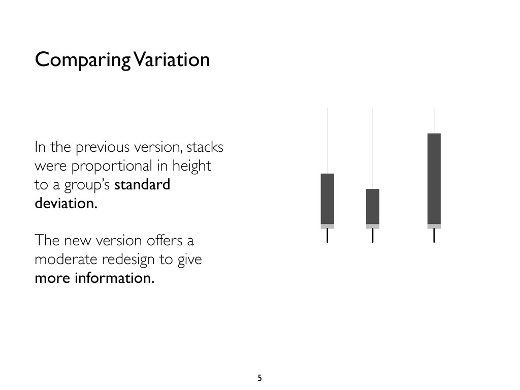
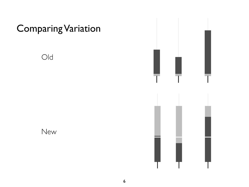
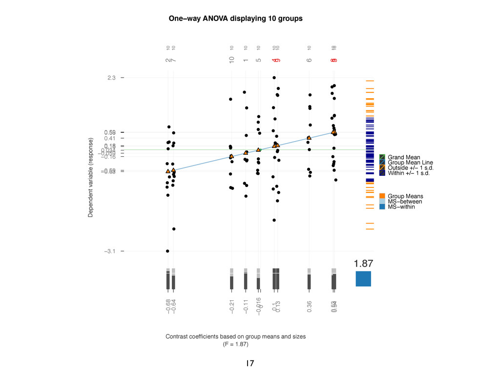
5. In the previous version, stacks were proportional in height to a group’s standard deviation. The new version offers a moderate redesign to give more information. Comparing Variation 5 • −0.067 −0.16 −0.14 0.088 −0.1 0.13 0.19 −0.15 0
6. Old Comparing Variation 6 ontrast coefficients based on group means and −0.067 −0.16 −0.14 0.088 −0.1 0.13 0.19 −0.15 0 • • • • • • • • • • • • • • • • • • • • 7 New
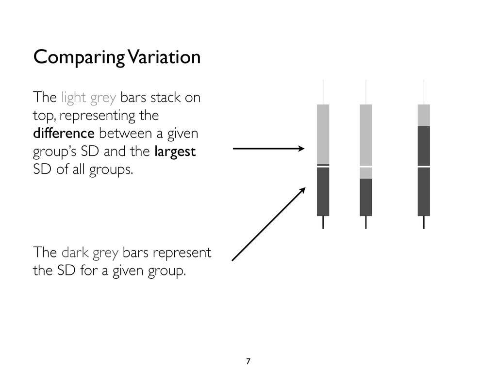
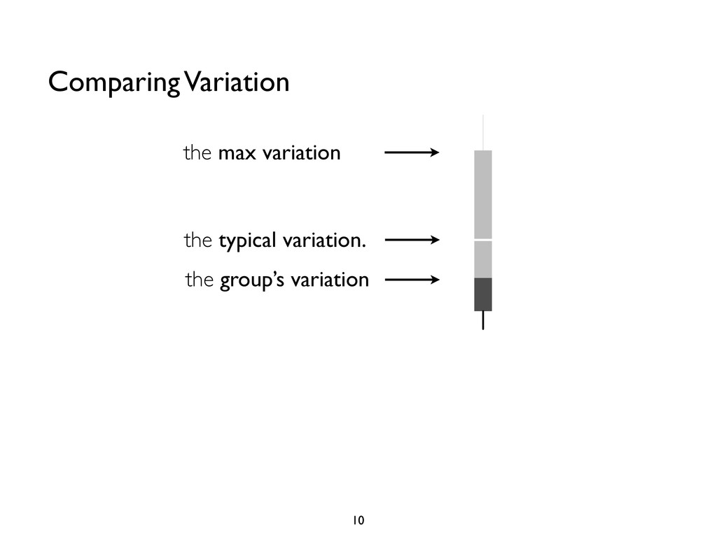
7. The dark grey bars represent the SD for a given group. Comparing Variation 7 The light grey bars stack on top, representing the difference between a given group’s SD and the largest SD of all groups. • −0.067 −0.16 −0.14 0.088 −0.1 0.13 0.19 −0.15 0
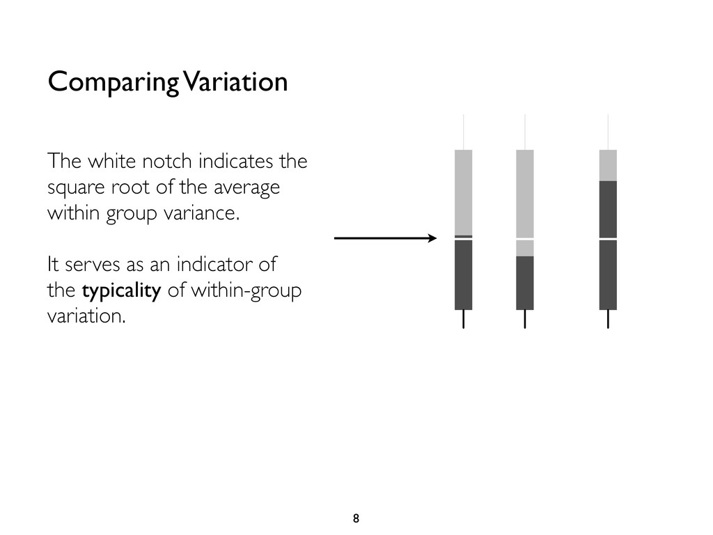
8. Comparing Variation 8 The white notch indicates the square root of the average within group variance. It serves as an indicator of the typicality of within-group variation. • −0.067 −0.16 −0.14 0.088 −0.1 0.13 0.19 −0.15 0
9. Comparing Variation 9 The advantage of the new design is that each group’s bar now contains more information. • −0.067 −0.16 −0.14 0.088 −0.1 0.13 0.19 −0.15 0
10. Comparing Variation 10 • • • • • • • • • −0.067 −0.16 −0.27 −0.14 −0.1 −0.24 −0.15 0 the group’s variation the typical variation. the max variation
11. Overplotting Logic 11 granova.1w.ggplot gives the user overplot information in both tabular and graphic form. • • • • • • • • • • • • • • • • • • • • • • • • • • • • • • • • • • • • • • • • • • • 1 1 5 6 4 9
12. Overplotting Logic 12 When groups are overplotted, granova. 1w.ggplot marks their group identifiers in red. −way ANOVA displaying 10 groups • • • • • • • • • • • • • • • 10 10 10 10 10 10 10 1 5 6 4 9
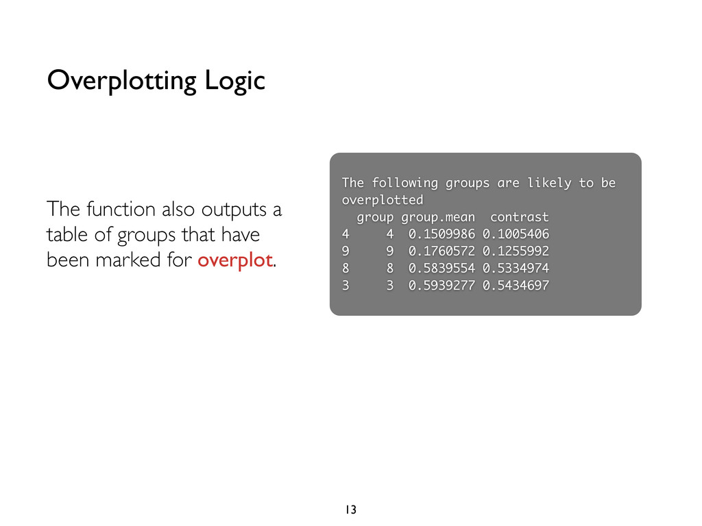
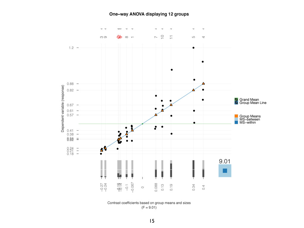
13. Overplotting Logic 13 The function also outputs a table of groups that have been marked for overplot. The following groups are likely to be overplotted group group.mean contrast 4 4 0.1509986 0.1005406 9 9 0.1760572 0.1255992 8 8 0.5839554 0.5334974 3 3 0.5939277 0.5434697
14. Sample Graphics granova.1w.ggplot() 14
15. 15 One−way ANOVA displaying 12 groups Contrast coefficients based on group means and sizes (F = 9.01) Dependent variable (response) 0.41 0.32 0.21 0.88 0.82 0.34 0.57 0.38 0.24 0.61 0.67 0.32 0.18 1.2 • • • • • • • • • • • • • • • • • • • • • • • • • • • • • • • • • • • • • • • • • • • • • • • • • 9.01 4 4 4 4 4 4 4 4 4 4 4 4 3 9 8 1 7 10 11 5 4 2 12 6 −0.067 −0.16 −0.27 0.4 0.34 −0.14 0.088 −0.1 −0.24 0.13 0.19 −0.15 0 • Grand Mean • Group Mean Line Group Means MS−between MS−within
16. 16 One−way ANOVA displaying 12 groups Contrast coefficients based on group means and sizes (F = 21.53) Dependent variable (response) 2.5 3.3 4.8 1.2 1.4 3 1.9 2.7 4.3 1.7 1.7 3.1 0.81 5.6 • • • • • • • • • • • • • • • • • • • • • • • • • • • • • • • • • • • • • • • • • • • • • • • • • 21.53 4 4 4 4 4 4 4 4 4 4 4 4 4 5 7 1 8 2 9 3 10 11 6 12 −0.14 0.65 2.2 −1.5 −1.2 0.41 −0.76 0.092 1.6 −0.93 −0.92 0.47 0 • Grand Mean • Group Mean Line Group Means MS−between MS−within
17. 17 One−way ANOVA displaying 10 groups Contrast coefficients based on group means and sizes (F = 1.87) Dependent variable (response) −0.059 −0.63 0.59 0.15 0.034 0.41 −0.59 0.58 0.18 −0.16 −3.1 2.3 • • • • • • • • • • • • • • • • • • • • • • • • • • • • • • • • • • • • • • • • • • • • • • • • • • • • • • • • • • • • • • • • • • • • • • • • • • • • • • • • • • • • • • • • • • • • • • • • • • • • • 1.87 10 10 10 10 10 10 10 10 10 10 2 7 10 1 5 6 4 9 8 3 −0.11 −0.68 0.54 0.1 −0.016 0.36 −0.64 0.53 0.13 −0.21 0 • Grand Mean • Group Mean Line • Outside +/− 1 s.d. • Within +/− 1 s.d. Group Means MS−between MS−within
18. 18 granova.1w() granova.2w() granova.contr() granova.ds()
19. Sample Graphics granova.contr  comparison 19
20. 20 granova.contr() • • • • • • • • • • • • • • • • • • • • • • • • • • • • • • • • • • • • • • • • • • • • • • • • • • • • • • • • • • • • −0.5 0.0 0.5 50 70 90 110 jitter(Xconss[, i][Xconss[, i] != 0], jj) Outcome (response) Coefficients vs. Response, Contrast .L • • • • • • • • • • • • • • • • • • • • • • • • • • • • • • • • • • • • • • • • • • • • • • • • • • • • • • • • • • • • • • −0.5 0.0 0.5 50 70 90 110 jitter(Xconss[, i][Xconss[, i] != 0], jj) Outcome (response) Coefficients vs. Response, Contrast .Q • • • • • • • • • • • • • • • • • • • • • • • • • • • • • • • • • • • • • • • • • • • • • • • • • • • • • • • • • • • • • • −0.5 0.0 0.5 50 70 90 110 jitter(Xconss[, i][Xconss[, i] != 0], jj) Outcome (response) Coefficients vs. Response, Contrast .C • • • • • • • • • • • • • • • • • • • • • • • • • • • • • • • • • • • • • • • • • • • • • • • • • • • • • • • • • • • • • • −0.5 0.0 0.5 50 70 90 110 jitter(Xconss[, i][Xconss[, i] != 0], jj) Outcome (response) Coefficients vs. Response, Contrast ^4 • •
21. 21 granova.contr.ggplot() Coefficients vs. Response Contrast .L Contrast .L Outcome (response) 50 60 70 80 90 100 110 120 • • • • • • • • • • • • • • • • • • • • • • • • • • • • • • • • • • • • • • • • • • • • • • • • • • • • • • • • • • • • −0.4 −0.2 0.0 0.2 0.4 Coefficients vs. Response Contrast .Q Contrast .Q Outcome (response) 50 60 70 80 90 100 110 120 • • • • • • • • • • • • • • • • • • • • • • • • • • • • • • • • • • • • • • • • • • • • • • • • • • • • • • • • • • • • −0.4 −0.2 0.0 0.2 0.4 Coefficients vs. Response Contrast .C Contrast .C Outcome (response) 50 60 70 80 90 100 110 120 • • • • • • • • • • • • • • • • • • • • • • • • • • • • • • • • • • • • • • • • • • • • • • • • • • • • • • • • • • • • −0.4 −0.2 0.0 0.2 0.4 Coefficients vs. Response Contrast ^4 Contrast ^4 Outcome (response) 50 60 70 80 90 100 110 120 • • • • • • • • • • • • • • • • • • • • • • • • • • • • • • • • • • • • • • • • • • • • • • • • • • • • • • • • • • • • −0.4 −0.2 0.0 0.2
22. 22 granova.contr.ggplot() • • • • • • • • • • • • • • • • • • • • • • • • • • • • • • • • • • • • • • • • • • • • • • • • • • • • • • • • • • • • −0.5 0.0 0.5 50 70 90 110 jitter(Xconss[, i][Xconss[, i] != 0], jj) Outcome (response) Coefficients vs. Response, Contrast .L • • • • • • • • • • • • • • • • • • • • • • • • • • • • • • • • • • • • • • • • • • • • • • • • • • • • • • • • • • • • • • −0.5 0.0 0.5 50 70 90 110 jitter(Xconss[, i][Xconss[, i] != 0], jj) Outcome (response) Coefficients vs. Response, Contrast .Q • • • • • • • • • • • • • • • • • • • • • • • • • • • • • • • • • • • • • • • • • • • • • • • • • • • • • • • • • • • • • • −0.5 0.0 0.5 50 70 90 110 jitter(Xconss[, i][Xconss[, i] != 0], jj) Outcome (response) Coefficients vs. Response, Contrast .C • • • • • • • • • • • • • • • • • • • • • • • • • • • • • • • • • • • • • • • • • • • • • • • • • • • • • • • • • • • • • • −0.5 0.0 0.5 50 70 90 110 jitter(Xconss[, i][Xconss[, i] != 0], jj) Outcome (response) Coefficients vs. Response, Contrast ^4 • • granova.contr() Coefficients vs. Response Contrast .L Contrast .L Outcome (response) 50 60 70 80 90 100 110 120 • • • • • • • • • • • • • • • • • • • • • • • • • • • • • • • • • • • • • • • • • • • • • • • • • • • • • • • • • • • • −0.4 −0.2 0.0 0.2 0.4 Coefficients vs. Response Contrast .Q Contrast .Q Outcome (response) 50 60 70 80 90 100 110 120 • • • • • • • • • • • • • • • • • • • • • • • • • • • • • • • • • • • • • • • • • • • • • • • • • • • • • • • • • • • • −0.4 −0.2 0.0 0.2 0.4 Coefficients vs. Response Contrast .C Contrast .C Outcome (response) 50 60 70 80 90 100 110 120 • • • • • • • • • • • • • • • • • • • • • • • • • • • • • • • • • • • • • • • • • • • • • • • • • • • • • • • • • • • • −0.4 −0.2 0.0 0.2 0.4 Coefficients vs. Response Contrast ^4 Contrast ^4 Outcome (response) 50 60 70 80 90 100 110 120 • • • • • • • • • • • • • • • • • • • • • • • • • • • • • • • • • • • • • • • • • • • • • • • • • • • • • • • • • • • • −0.4 −0.2 0.0 0.2
23. 23 granova.contr.ggplot() granova.contr() ) rast ^5 • • • • • • • • • • • • • • • • • • • • • • • • • • • • • • • • • • • • • • • • • • • • • • • • • • • • • • • • • • • • Group Indicator Outcome (response) • • • • • • 1 2 3 4 5 6 50 70 90 110 Responses for all groups, each n= 10 Coefficients vs. Response Contrast ^5 Contrast ^5 Outcome (response) 50 60 70 80 90 100 110 120 • • • • • • • • • • • • • • • • • • • • • • • • • • • • • • • • • • • • • • • • • • • • • • • • • • • • • • • • • • • • −0.6 −0.4 −0.2 0.0 0.2 0.4 0.6 Responses for all groups each n = 10 Group Indicator Outcome (response) 50 60 70 80 90 100 110 120 • • • • • • • • • • • • • • • • • • • • • • • • • • • • • • • • • • • • • • • • • • • • • • • • • • • • • • • • • • • • • • • • • • 1 2 3 4 5 6
24. 24 Take it for a spin yourself Step 1: Step 2: $> cd [where you want to put the granova folder] $> git clone git@github.com:briandk/granova.git get git: http://git-scm.com/ Step 3: set your R working directory to granova Step 4: R> source("inst/dev.R", chdir = TRUE) Terminal R Console