granovaGG20110224

A first-pass overview at granovaGG and the one-way function

Transcript

1. Developing  granova A ggplot2 package for graphical Analysis of Variance DC UseR Meetup – February 24, 2011 Brian Danielak briandk@umd.edu 1
2. j.mp/granovaDev 2
3. 3 granova is a package of four functions created by Robert Pruzek and James Helmreich granova.1w() granova.2w() granova.contr() granova.ds() http://cran.r-project.org/web/packages/granova/
4. 4 Today we’re looking at this one granova.1w() granova.2w() granova.contr() granova.ds()
5. Let’s say you’ve got some some data that’s just begging to be analyzed by ANOVA. 5
6. Think out loud for a moment with me. Let’s build up a visualization for ANOVA. 6
7. 7 red green blue 3 Treatments 9 participants per cell
8. 8 Suppose we took all the scores and looked at them like a univariate strip chart. Scores (N = 27)
9. 9 Then suppose we rotated it 90°
10. 10 So here’s our rotated univariate strip chart
11. 11 These are the blue treatments
12. 12 These are the red treatments
13. 13 Let’s try something fun with our univariate distribution
14. 14 Suppose I started making a graph 0
15. 15 Suppose I started making a graph 0 score
16. 16 For funsies, I’m going to plop our univariate strip chart at zero 0 score Scores (N = 27)
17. 17 Let’s look at just the red treatments. 0 score
18. 18 What if we started exploiting the x-dimension... 0 score
19. 19 ...By shoving this group off-zero by some amount? 0 score
20. 20 0 score ...By shoving this group off-zero by some amount?
21. ZOMG It’s Math TIME 21
22. ZOMG It’s Math TIME (Hide teh childrens!!!) 22
23. Let’s define the direction and magnitude of the “shove” for each group as follows: 23
24. shove = group mean - grand mean 24 Let’s define the direction and magnitude of the “shove” for each group as follows:
25. shove = group mean - grand mean (See? That wasn’t so bad. But it’s still ok to cry if you need to.) 25 Let’s define the direction and magnitude of the “shove” for each group as follows:
26. 26 0 score shove shove  =  mean(red)      -­‐  grand.mean
27. 27 0 score shove shove  =  mean(red)      -­‐  grand.mean
28. 28 shove  =  mean(red)      -­‐  grand.mean shove  =  mean(blue)    -­‐  grand.mean 0 score shove shove
29. 29 0 score shove shove shove  =  mean(red)      -­‐  grand.mean shove  =  mean(blue)    -­‐  grand.mean
30. shove 30 0 score shove shove shove  =  mean(red)      -­‐  grand.mean shove  =  mean(blue)    -­‐  grand.mean shove  =  mean(green)  -­‐  grand.mean
31. 31 shove 0 score shove shove There’s a subtle advantage to computing our shoves this way.
32. 32 shove 0 shove Because if you think about it
33. 33 shove 0 shove shove = group mean - grand mean shove = the main effect for a group
34. 34 main effect 0 main effect shove = group mean - grand mean shove = the main effect for a group
35. 35 Building the graphic this way lets us read off the main effects values easily. main effect 0 score main effect main effect
36. What should an ANOVA graphic have? 36
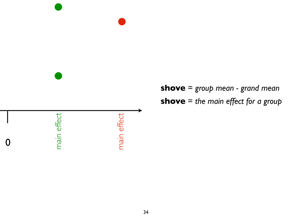
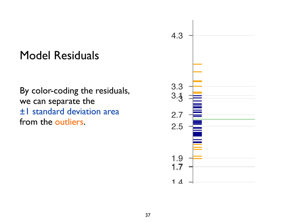
37. Dependent variable (response) 2.5 3.3 4.8 1.2 1.4 3 1.9 2.7 4.3 1.7 1.7 3.1 0.8 • • • • • • • • • • • • • • • • By color-coding the residuals, we can separate the ±1 standard deviation area from the outliers. Model Residuals 37
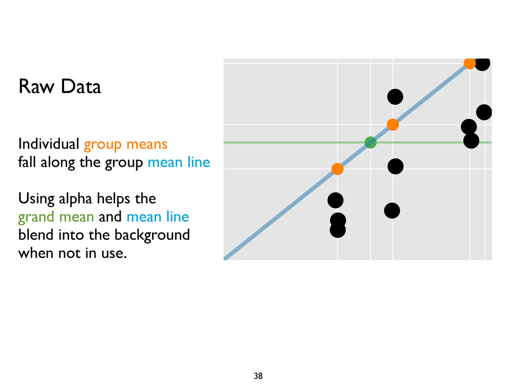
38. Individual group means fall along the group mean line Using alpha helps the grand mean and mean line blend into the background when not in use. • • • • • • • • • • • • • • • • • • • • • • • • • • • • • • • • • • • • Raw Data 38
39. We represent MS-between and MS-within as opaque squares. The ratio of their areas is generated by the F-statistic itself. 6.58 2.2 1.6 F-Statistic 39
40. We can then use the space above the squares for more information. Here, I’vecalculated Cohen’s f^2 for effect size. F2 = R2 1 − R2 6.58 2.2 1.6 40 Effect Size
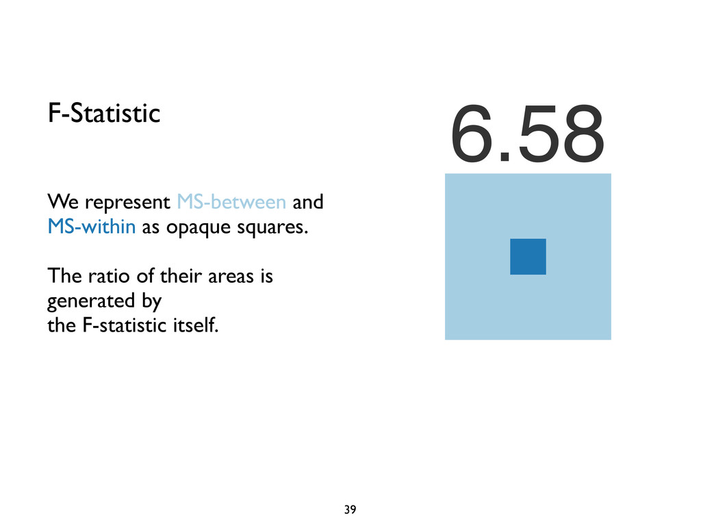
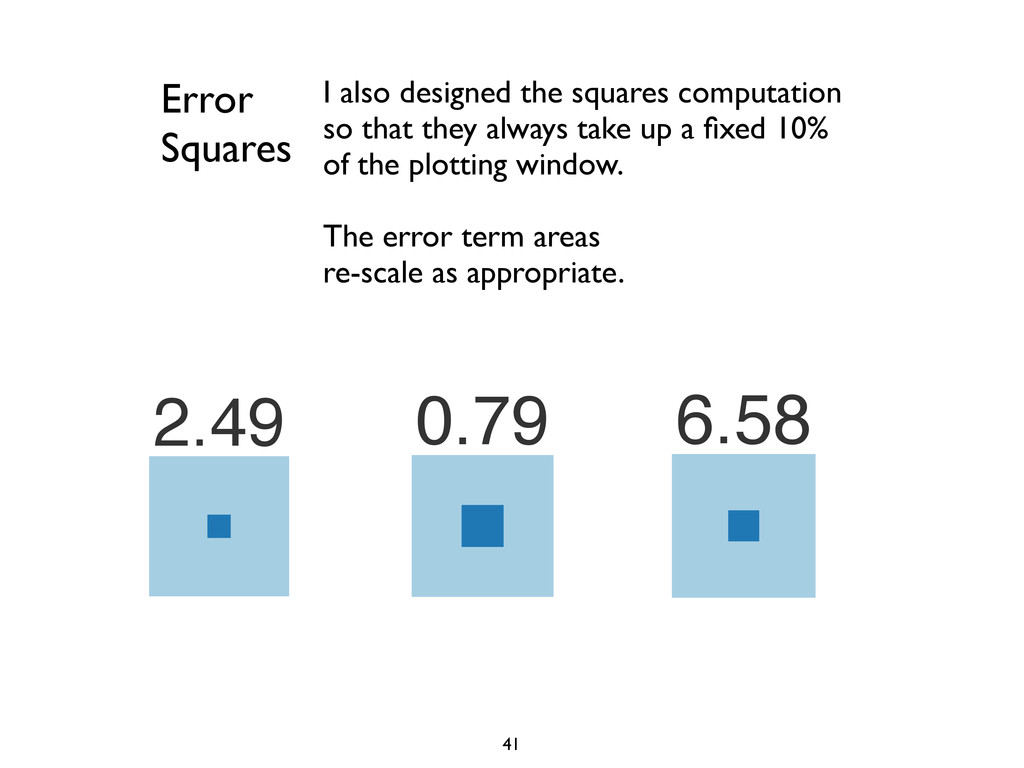
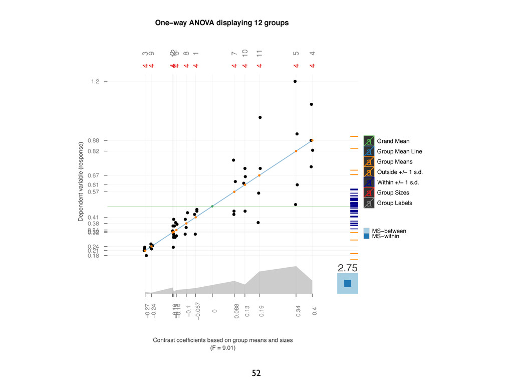
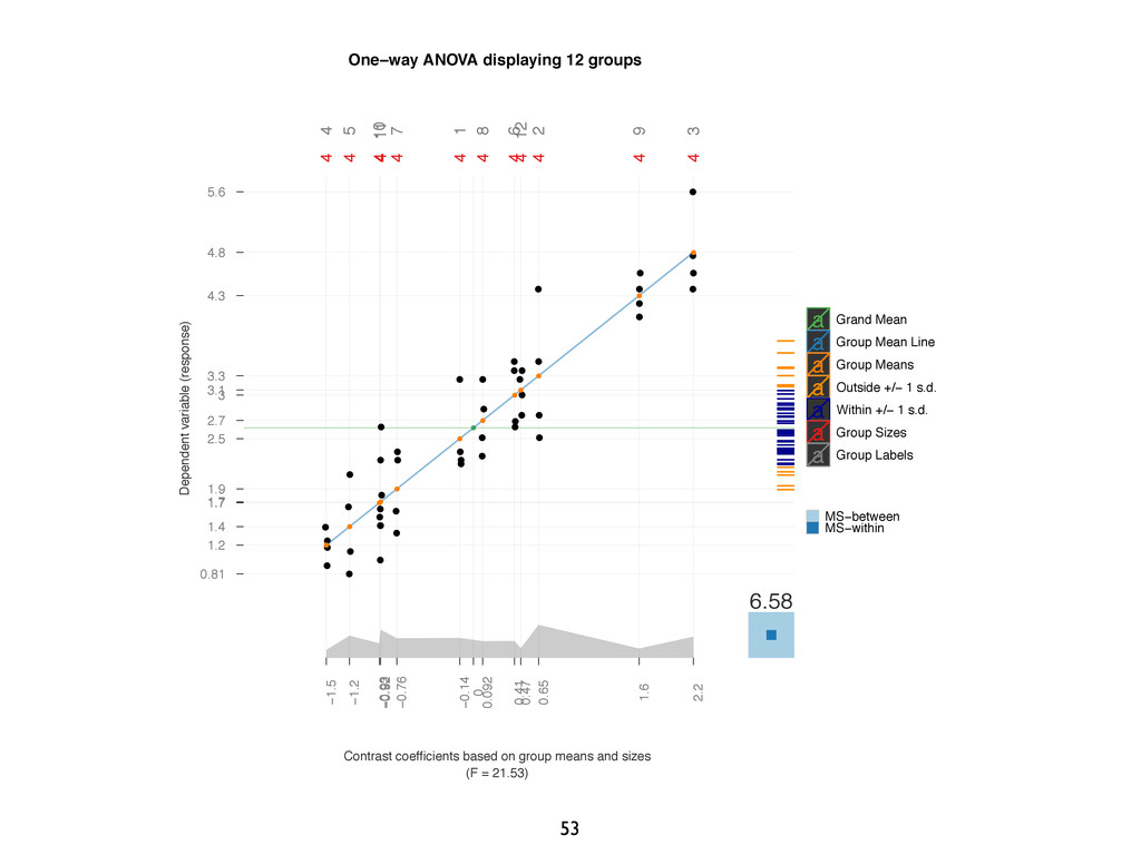
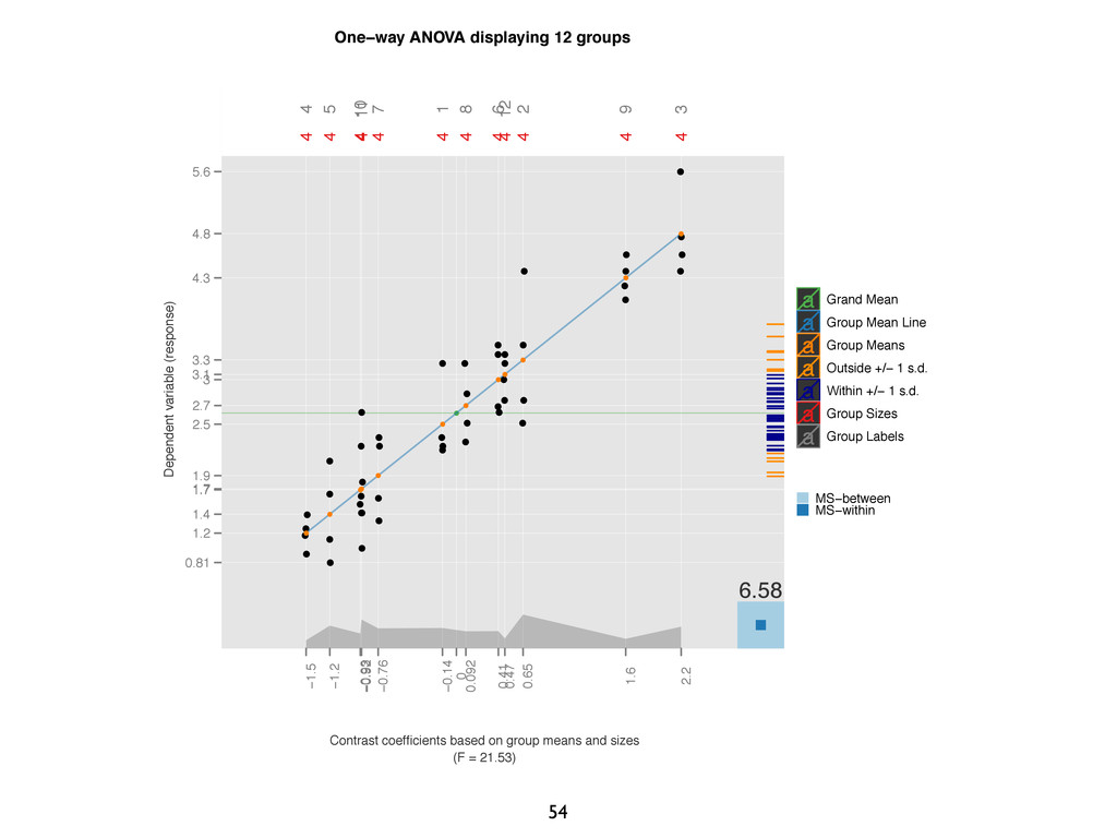
41. I also designed the squares computation so that they always take up a fixed 10% of the plotting window. The error term areas re-scale as appropriate. 0.79 29 49 MS−between MS−within 2.49 63 MS−between MS−within 6.58 0.65 2.2 1.6 MS−be MS−w 41 Error Squares
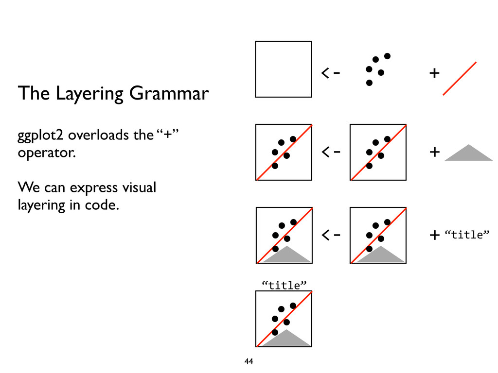
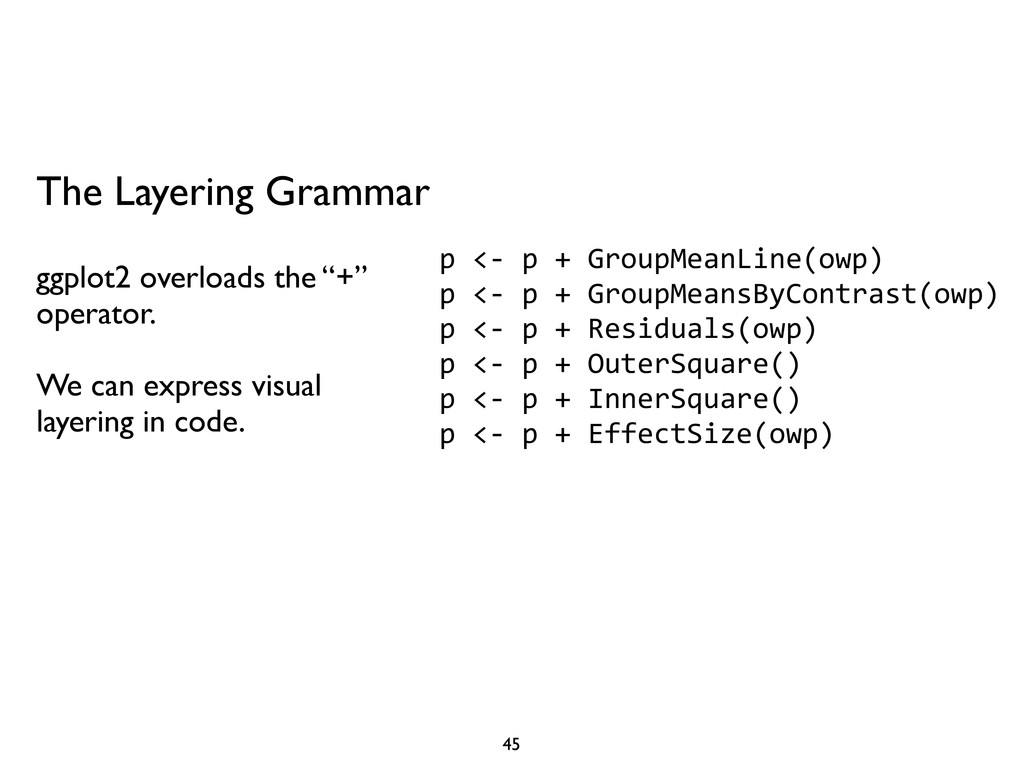
42. And, we can use color schemes to alert viewers to information. Here, error squares turn red when the F-statistic < 1 0.79 29 49 MS−between MS−within 42 • • • • 0.07 0.27 0.49 0.11 0.14 MS−w MS−be Error Squares
43. We created a ribbon whose height is proportional to each group’s standard deviation. Comparing Variation Contrast coefficients based on group means and sizes (F = 0.53) • • • • • • • • • • • • • 0.27 −0.5 −0.23 −0.31 0.11 0.036 0.14 0 43
44. ggplot2 overloads the “+” operator. We can express visual layering in code. The Layering Grammar + <-­‐ <-­‐ + + <-­‐ “title” “title” 44
45. ggplot2 overloads the “+” operator. We can express visual layering in code. The Layering Grammar p  <-­‐  p  +  GroupMeanLine(owp) p  <-­‐  p  +  GroupMeansByContrast(owp) p  <-­‐  p  +  Residuals(owp) p  <-­‐  p  +  OuterSquare() p  <-­‐  p  +  InnerSquare() p  <-­‐  p  +  EffectSize(owp) 45
46. A Sample Function GroupMeansByContrast  <-­‐  function(owp)  {    return(          geom_point(                            aes(                              x          =  contrast,                                y          =  group.mean,                                color  =  factor("Group  Means")                          ),                              size    =  I(3/2),                              data    =  owp$summary,          )    ) } 46
47. Value = Key GetColors  <-­‐  function()  {    colors  <-­‐  c(      GetMSbetweenColor(owp),      GetMSwithinColor(owp),      brewer.pal(n  =  8,  name  =  "Set1")[3],      brewer.pal(n  =  8,  name  =  "Paired")[8],      brewer.pal(n  =  8,  name  =  "Paired")[2],      "darkblue",    )    names(colors)  <-­‐  c(        "MS-­‐between",        "MS-­‐within",        "Grand  Mean",        "Group  Means",        "Group  Mean  Line",        "Within  +/-­‐  1  s.d.",    )    return(colors) } 47
48. GetColors  <-­‐  function()  {    colors  <-­‐  c(      GetMSbetweenColor(owp),      GetMSwithinColor(owp),      brewer.pal(n  =  8,  name  =  "Set1")[3],      brewer.pal(n  =  8,  name  =  "Paired")[8],      brewer.pal(n  =  8,  name  =  "Paired")[2],      "darkblue",    )    names(colors)  <-­‐  c(        "MS-­‐between",        "MS-­‐within",        "Grand  Mean",        "Group  Means",        "Group  Mean  Line",        "Within  +/-­‐  1  s.d.",    )    return(colors) } 48 The Beauty of Color ColorScale  <-­‐  function(owp)  {    return(        scale_color_manual(            value  =  owp$colors,  name  =  "")    ) } p  <-­‐  p  +  ColorScale(owp)
49. Connecting with plyr 49
50. plyr + ggplot = <3 GetSummary  <-­‐  function(owp)  {    return(        ddply(owp$data,  .(group),  summarise,            group                            =  unique(group),            group.mean                  =  mean(score),            contrast                      =  unique(contrast),            variance                      =  var(score),            standard.deviation  =  sd(score),            maximum.score            =  max(score),            group.size                  =  length(score)        )    ) } 50
51. Sample Graphics 51
52. One−way ANOVA displaying 12 groups Contrast coefficients based on group means and sizes (F = 9.01) Dependent variable (response) 0.41 0.32 0.21 0.88 0.82 0.34 0.57 0.38 0.24 0.61 0.67 0.32 0.18 1.2 • • • • • • • • • • • • • • • • • • • • • • • • • • • • • • • • • • • • • • • • • • • • • • • • • • • • • • • • • • • • • 2.75 4 4 4 4 4 4 4 4 4 4 4 4 1 2 3 4 5 6 7 8 9 10 11 12 −0.067 −0.16 −0.27 0.4 0.34 −0.14 0.088 −0.1 −0.24 0.13 0.19 −0.15 0 • • a a Grand Mean • • a a Group Mean Line • • a a Group Means • • a a Outside +/− 1 s.d. • • a a Within +/− 1 s.d. • • a a Group Sizes • • a a Group Labels MS−between MS−within 52
53. One−way ANOVA displaying 12 groups Contrast coefficients based on group means and sizes (F = 21.53) Dependent variable (response) 2.5 3.3 4.8 1.2 1.4 3 1.9 2.7 4.3 1.7 1.7 3.1 0.81 5.6 • • • • • • • • • • • • • • • • • • • • • • • • • • • • • • • • • • • • • • • • • • • • • • • • • • • • • • • • • • • • • 6.58 4 4 4 4 4 4 4 4 4 4 4 4 1 2 3 4 5 6 7 8 9 10 11 12 −0.14 0.65 2.2 −1.5 −1.2 0.41 −0.76 0.092 1.6 −0.93 −0.92 0.47 0 • • a a Grand Mean • • a a Group Mean Line • • a a Group Means • • a a Outside +/− 1 s.d. • • a a Within +/− 1 s.d. • • a a Group Sizes • • a a Group Labels MS−between MS−within 53
54. 54 One−way ANOVA displaying 12 groups Contrast coefficients based on group means and sizes (F = 21.53) Dependent variable (response) 2.5 3.3 4.8 1.2 1.4 3 1.9 2.7 4.3 1.7 1.7 3.1 0.81 5.6 • • • • • • • • • • • • • • • • • • • • • • • • • • • • • • • • • • • • • • • • • • • • • • • • • • • • • • • • • • • • • 6.58 4 4 4 4 4 4 4 4 4 4 4 4 1 2 3 4 5 6 7 8 9 10 11 12 −0.14 0.65 2.2 −1.5 −1.2 0.41 −0.76 0.092 1.6 −0.93 −0.92 0.47 0 • • a a Grand Mean • • a a Group Mean Line • • a a Group Means • • a a Outside +/− 1 s.d. • • a a Within +/− 1 s.d. • • a a Group Sizes • • a a Group Labels MS−between MS−within
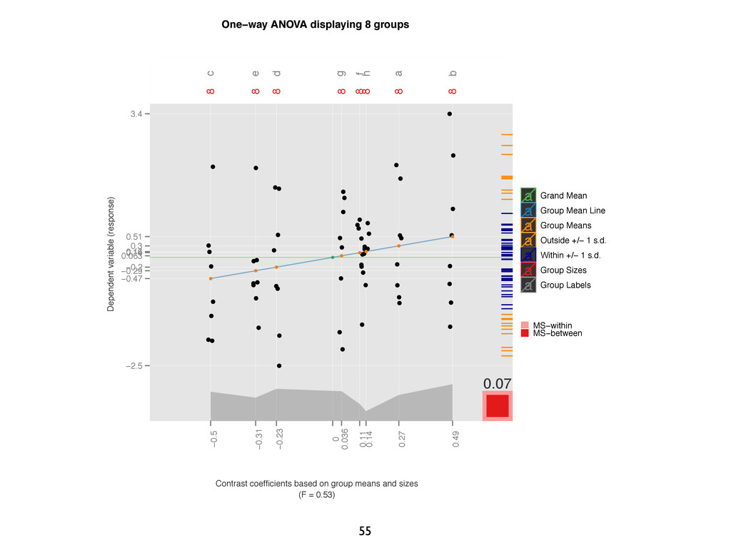
55. 55 One−way ANOVA displaying 8 groups Contrast coefficients based on group means and sizes (F = 0.53) Dependent variable (response) 0.3 0.51 −0.47 −0.2 −0.29 0.14 0.063 0.16 −2.5 3.4 • • • • • • • • • • • • • • • • • • • • • • • • • • • • • • • • • • • • • • • • • • • • • • • • • • • • • • • • • • • • • • • • • • • • • • • • • 0.07 8 8 8 8 8 8 8 8 a b c d e f g h 0.27 0.49 −0.5 −0.23 −0.31 0.11 0.036 0.14 0 • • a a Grand Mean • • a a Group Mean Line • • a a Group Means • • a a Outside +/− 1 s.d. • • a a Within +/− 1 s.d. • • a a Group Sizes • • a a Group Labels MS−within MS−between
56. 56 Thank You! (please send me coupons) briandk@umd.edu @Capbri