Advanced Topics in EXAFS Analysis

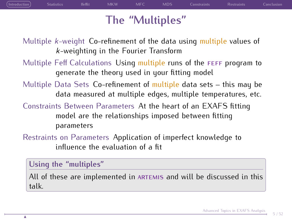
This talk is an overview of advanced practice in EXAFS analysis as implemented in Ifeffit and Artemis. This includes a discussion of statistics in the EXAFS fit and the application of multiple data sets, multiple Feff calculations, and multiple k-weighting. It also provides examples of constraints and restraints as implemented in our software.

Transcript

1. Introduction Statistics Ifeffit MKW MFC MDS Constraints Restraints Conclusion Advanced Topics in EXAFS Analysis Bruce Ravel Synchrotron Methods Group, Ceramics Division Materials Measurement Laboratory National Institute of Standards and Technology & Local Contact, Beamline X23A2 National Synchrotron Light Source EXAFS Data Analysis workshop 2011 Diamond Light Source November 14–17, 2011 1 / 52 Advanced Topics in EXAFS Analysis
2. Introduction Statistics Ifeffit MKW MFC MDS Constraints Restraints Conclusion Copyright This document is copyright c 2010-2011 Bruce Ravel. This work is licensed under the Creative Commons Attribution-ShareAlike License. To view a copy of this license, visit http://creativecommons.org/licenses/by-sa/3.0/ or send a letter to Creative Commons, 559 Nathan Abbott Way, Stanford, California 94305, USA. You are free: to Share  to copy, distribute, and transmit the work to Remix  to adapt the work to make commercial use of the work Under the following conditions: Attribution – You must attribute the work in the manner specified by the author or licensor (but not in any way that suggests that they endorse you or your use of the work). Share Alike – If you alter, transform, or build upon this work, you may distribute the resulting work only under the same, similar or a compatible license. With the understanidng that: Waiver – Any of the above conditions can be waived if you get permission from the copyright holder. Public Domain – Where the work or any of its elements is in the public domain under applicable law, that status is in no way affected by the license. Other Rights – In no way are any of the following rights affected by the license: Your fair dealing or fair use rights, or other applicable copyright exceptions and limitations; The author’s moral rights; Rights other persons may have either in the work itself or in how the work is used, such as publicity or privacy rights. Notice – For any reuse or distribution, you must make clear to others the license terms of this work. This is a human-readable summary of the Legal Code (the full license). 2 / 52 Advanced Topics in EXAFS Analysis
3. Introduction Statistics Ifeffit MKW MFC MDS Constraints Restraints Conclusion Acknowledgments Matt Newville, of course. Without none of us would be having this much fun Shelly Kelly, bug finder extraordinaire and progenitor of several examples in this talk John Rehr and his group. If we didn’t have fun with , we wouldn’t have fun with Ed Stern, for teaching us all so well and for getting all this XAS stuff started in the first place The many users of my software: without years of feedback and encouragement, my codes would suck way more than they do The folks who make the great software I use to write my codes: Perl, wxPerl, Emacs, The Emacs Code Browser, Git, GitHub The folks who make the great software used to write this talk: L ATEX, Beamer, Avogadro, The Gimp, Gnuplot 3 / 52 Advanced Topics in EXAFS Analysis
4. Introduction Statistics Ifeffit MKW MFC MDS Constraints Restraints Conclusion This Talk This is NOT the introductory talk I assume you are a veteran of many XAS campaigns and that you already have your own data that you care about. I assume you are familiar with the EXAFS equation. I assume you understand XAS data processing and have done some EXAFS analysis. Some familiarity with or will help. The audience for this talk is interested in advanced techniques which will improve their use of their EXAFS data. 4 / 52 Advanced Topics in EXAFS Analysis
5. Introduction Statistics Ifeffit MKW MFC MDS Constraints Restraints Conclusion The “Multiples” Multiple k-weight Co-refinement of the data using multiple values of k-weighting in the Fourier Transform Multiple Feff Calculations Using multiple runs of the program to generate the theory used in your fitting model Multiple Data Sets Co-refinement of multiple data sets – this may be data measured at multiple edges, multiple temperatures, etc. Constraints Between Parameters At the heart of an EXAFS fitting model are the relationships imposed between fitting parameters Restraints on Parameters Application of imperfect knowledge to influence the evaluation of a fit Using the “multiples” All of these are implemented in and will be discussed in this talk. 5 / 52 Advanced Topics in EXAFS Analysis
6. Introduction Statistics Ifeffit MKW MFC MDS Constraints Restraints Conclusion Information Content of EXAFS (I) Sometimes, we have beautiful data. This is the merge of 5 scans on a 50 nm film of GeSb on silica, at the Ge edge and measured in fluorescence at NSLS X23A2. Here, I show a Fourier transform window of [3 : 13] and I suggest a fitting range of [1.7 : 4.7]. Applying the Nyquist criterion: Nidp ≈ 2∆k∆R π ≈ 19 This gives us an upper bound of the information content of that portion of the EXAFS spectrum. 6 / 52 Advanced Topics in EXAFS Analysis These data are courtesy of Joseph Washington and Eric Joseph (IBM Research)
7. Introduction Statistics Ifeffit MKW MFC MDS Constraints Restraints Conclusion Information Content of EXAFS (II) Sometimes, we have less-than-beautiful data. This is the merge of 42 scans on a solution containing 3 mM of Hg bound to a synthetic DNA complex, measured in fluorescence at APS 20BM. Here, I show a Fourier transform window of [2 : 8.8] and I suggest a fitting range of [1 : 3]. Applying the Nyquist criterion: Nidp ≈ 2∆k∆R π ≈ 8 This talk discusses strategies for dealing with severely limited information content. 7 / 52 Advanced Topics in EXAFS Analysis B. Ravel, et al., EXAFS studies of catalytic DNA sensors for mercury contamination of water, Radiation Physics and Chemistry 78:10 (2009) pp S75-S79. DOI:10.1016/j.radphyschem.2009.05.024
8. Introduction Statistics Ifeffit MKW MFC MDS Constraints Restraints Conclusion What is This Nyquist Criterion thingie? Applying Fourier analysis to χ(k) means that we treat EXAFS as a signal processing problem. If The signal is ideally packed and 8 / 52 Advanced Topics in EXAFS Analysis
9. Introduction Statistics Ifeffit MKW MFC MDS Constraints Restraints Conclusion What is This Nyquist Criterion thingie? Applying Fourier analysis to χ(k) means that we treat EXAFS as a signal processing problem. If The signal is ideally packed and The error in the fitting parameters is normally distributed and 8 / 52 Advanced Topics in EXAFS Analysis
10. Introduction Statistics Ifeffit MKW MFC MDS Constraints Restraints Conclusion What is This Nyquist Criterion thingie? Applying Fourier analysis to χ(k) means that we treat EXAFS as a signal processing problem. If The signal is ideally packed and The error in the fitting parameters is normally distributed and We understand and can enumerate all sources of error and 8 / 52 Advanced Topics in EXAFS Analysis
11. Introduction Statistics Ifeffit MKW MFC MDS Constraints Restraints Conclusion What is This Nyquist Criterion thingie? Applying Fourier analysis to χ(k) means that we treat EXAFS as a signal processing problem. If The signal is ideally packed and The error in the fitting parameters is normally distributed and We understand and can enumerate all sources of error and We know the theoretical lineshape of our data then 8 / 52 Advanced Topics in EXAFS Analysis
12. Introduction Statistics Ifeffit MKW MFC MDS Constraints Restraints Conclusion What is This Nyquist Criterion thingie? Applying Fourier analysis to χ(k) means that we treat EXAFS as a signal processing problem. If The signal is ideally packed and The error in the fitting parameters is normally distributed and We understand and can enumerate all sources of error and We know the theoretical lineshape of our data then Nidp ≈ 2∆k∆R π where, for EXAFS, ∆k is the range of Fourier transform and ∆R is the range in R over which the fit is evaluated. 8 / 52 Advanced Topics in EXAFS Analysis
13. Introduction Statistics Ifeffit MKW MFC MDS Constraints Restraints Conclusion What is This Nyquist Criterion thingie? Applying Fourier analysis to χ(k) means that we treat EXAFS as a signal processing problem. If The signal is ideally packed and The error in the fitting parameters is normally distributed and We understand and can enumerate all sources of error and We know the theoretical lineshape of our data then Nidp ≈ 2∆k∆R π where, for EXAFS, ∆k is the range of Fourier transform and ∆R is the range in R over which the fit is evaluated. Unfortunately ... None of those conditions really get met in EXAFS. Nidp is, at best, an upper bond of the actual information content of the EXAFS signal. 8 / 52 Advanced Topics in EXAFS Analysis
14. Introduction Statistics Ifeffit MKW MFC MDS Constraints Restraints Conclusion Statistical Parameters: Definitions uses a Levenberg-Marquardt non-linear least-squares minimization, a standard χ2 fitting metric, and a simple definition of an R-factor: χ2 = Nidp Ndata max i=min Re χd (ri ) − χt (ri ) 2 + Im χd (ri ) − χt (ri ) 2 (1) χ2 ν = χ2 ν (2) ν = Nidp − Nvar (3) = measurement uncertainty R = max i=min Re χd (ri ) − χt (ri ) 2 + Im χd (ri ) − χt (ri ) 2 max i=min Re χd (ri ) 2 + Im χd (ri ) 2 (4) In Gaussian statistics, assuming that has been measured correctly, a good fit has χ2 ν ≈ 1. 9 / 52 Advanced Topics in EXAFS Analysis
15. Introduction Statistics Ifeffit MKW MFC MDS Constraints Restraints Conclusion An Obviously Good Fit Here is a fit to the first two shells of copper metal at 10 K This is an unambiguously good fit: R 0.012 Nidp 16 ν 12 S2 0 0.87(6) E0 6.04(62) eV a 3.6063(49) ˚ A ΘD 550(46) K 10 / 52 Advanced Topics in EXAFS Analysis
16. Introduction Statistics Ifeffit MKW MFC MDS Constraints Restraints Conclusion An Obviously Good Fit Here is a fit to the first two shells of copper metal at 10 K This is an unambiguously good fit: R 0.012 Nidp 16 ν 12 S2 0 0.87(6) E0 6.04(62) eV a 3.6063(49) ˚ A ΘD 550(46) K Yet χ2 ν = 227.8 ! What’s goin’ on here? Why is χ2 ν for an obviously good fit so much larger than 1? 10 / 52 Advanced Topics in EXAFS Analysis
17. Introduction Statistics Ifeffit MKW MFC MDS Constraints Restraints Conclusion Statistical Parameters: Fit Evaluation The determination of measurement uncertainty is, perhaps, a bit hokey in . It is the average of the signal between 15 ˚ A and 25 ˚ A in the Fourier transform – a range that probably does not include much signal above the noise. Is that signal between 15 ˚ A and 25 ˚ A in copper metal? Perhaps.... In any case, this method ignores the following: Approximations and errors in theory Sample inhomogeneity Detector non-linearity Gremlins  never forget about the gremlins! ¨ 11 / 52 Advanced Topics in EXAFS Analysis
18. Introduction Statistics Ifeffit MKW MFC MDS Constraints Restraints Conclusion Statistical Parameters: Interpretation I OK then ... what is the implication of never being evaluated correctly by ? 1 χ2 ν is always somewhere between big and enormous. 12 / 52 Advanced Topics in EXAFS Analysis
19. Introduction Statistics Ifeffit MKW MFC MDS Constraints Restraints Conclusion Statistical Parameters: Interpretation I OK then ... what is the implication of never being evaluated correctly by ? 1 χ2 ν is always somewhere between big and enormous. 2 χ2 ν is impossible to interpret for a single fit. 12 / 52 Advanced Topics in EXAFS Analysis
20. Introduction Statistics Ifeffit MKW MFC MDS Constraints Restraints Conclusion Statistical Parameters: Interpretation I OK then ... what is the implication of never being evaluated correctly by ? 1 χ2 ν is always somewhere between big and enormous. 2 χ2 ν is impossible to interpret for a single fit. 3 χ2 ν can be used to compare different fits. A fit is improved if χ2 ν is significantly smaller. 12 / 52 Advanced Topics in EXAFS Analysis
21. Introduction Statistics Ifeffit MKW MFC MDS Constraints Restraints Conclusion Statistical Parameters: Interpretation I OK then ... what is the implication of never being evaluated correctly by ? 1 χ2 ν is always somewhere between big and enormous. 2 χ2 ν is impossible to interpret for a single fit. 3 χ2 ν can be used to compare different fits. A fit is improved if χ2 ν is significantly smaller. 4 Error bars are taken from the diagonal of the covariance matrix. If χ2 ν is way too big, the error bars will be way too small. The error bars reported by have been scaled by χ2 ν . 12 / 52 Advanced Topics in EXAFS Analysis
22. Introduction Statistics Ifeffit MKW MFC MDS Constraints Restraints Conclusion Statistical Parameters: Interpretation I OK then ... what is the implication of never being evaluated correctly by ? 1 χ2 ν is always somewhere between big and enormous. 2 χ2 ν is impossible to interpret for a single fit. 3 χ2 ν can be used to compare different fits. A fit is improved if χ2 ν is significantly smaller. 4 Error bars are taken from the diagonal of the covariance matrix. If χ2 ν is way too big, the error bars will be way too small. The error bars reported by have been scaled by χ2 ν . 5 Thus the error bars reported by are of the “correct” size if we assume that the fit is a “good fit”. 12 / 52 Advanced Topics in EXAFS Analysis
23. Introduction Statistics Ifeffit MKW MFC MDS Constraints Restraints Conclusion Statistical Parameters: Interpretation II How do we know if a fit is “good”? The current fit is an improvement over the previous fit if χ2 ν is sufficiently smaller. 13 / 52 Advanced Topics in EXAFS Analysis
24. Introduction Statistics Ifeffit MKW MFC MDS Constraints Restraints Conclusion Statistical Parameters: Interpretation II How do we know if a fit is “good”? The current fit is an improvement over the previous fit if χ2 ν is sufficiently smaller. You should be suspicious of a fit for which Nvar is close to Nidp, i.e. a fit for which ν is small. 13 / 52 Advanced Topics in EXAFS Analysis
25. Introduction Statistics Ifeffit MKW MFC MDS Constraints Restraints Conclusion Statistical Parameters: Interpretation II How do we know if a fit is “good”? The current fit is an improvement over the previous fit if χ2 ν is sufficiently smaller. You should be suspicious of a fit for which Nvar is close to Nidp, i.e. a fit for which ν is small. All variable parameters should have values that are physically defensible and error bars that make sense. 13 / 52 Advanced Topics in EXAFS Analysis
26. Introduction Statistics Ifeffit MKW MFC MDS Constraints Restraints Conclusion Statistical Parameters: Interpretation II How do we know if a fit is “good”? The current fit is an improvement over the previous fit if χ2 ν is sufficiently smaller. You should be suspicious of a fit for which Nvar is close to Nidp, i.e. a fit for which ν is small. All variable parameters should have values that are physically defensible and error bars that make sense. The results should be consistent with other things you know about the sample. 13 / 52 Advanced Topics in EXAFS Analysis
27. Introduction Statistics Ifeffit MKW MFC MDS Constraints Restraints Conclusion Statistical Parameters: Interpretation II How do we know if a fit is “good”? The current fit is an improvement over the previous fit if χ2 ν is sufficiently smaller. You should be suspicious of a fit for which Nvar is close to Nidp, i.e. a fit for which ν is small. All variable parameters should have values that are physically defensible and error bars that make sense. The results should be consistent with other things you know about the sample. The R-factor should be small and the fit should closely over-plot the data. (That was redundant. ¨ ) 13 / 52 Advanced Topics in EXAFS Analysis
28. Introduction Statistics Ifeffit MKW MFC MDS Constraints Restraints Conclusion Interpreting Error Bars The interpretation of an error bar depends on the meaning of the parameter. A fitted σ2 value of, say, 0.00567 ± 0.00654 is troubling. That result means that σ2 is ill-determined for that path and not even positive definite. Yikes! 14 / 52 Advanced Topics in EXAFS Analysis
29. Introduction Statistics Ifeffit MKW MFC MDS Constraints Restraints Conclusion Interpreting Error Bars The interpretation of an error bar depends on the meaning of the parameter. A fitted σ2 value of, say, 0.00567 ± 0.00654 is troubling. That result means that σ2 is ill-determined for that path and not even positive definite. Yikes! On the other hand, a fitted E0 value of, say, 0.12 ± 0.34 is just fine. E0 can be positive or negative. A fitted value consistent with 0 suggests you chose E0 wisely back in . 14 / 52 Advanced Topics in EXAFS Analysis
30. Introduction Statistics Ifeffit MKW MFC MDS Constraints Restraints Conclusion Outside Knowledge Because the information content of the XAS measurement is so limited, we are forced to incorporate knowledge from other measurements into our data analysis and its interpretation. Other XAS measurements  for instance, the “chemical transferability” of S2 0 Diffraction tells us structure, coordination number, bond lengths, etc. Things like NMR, UV/Vis, and IR can tell us about the ligation environment of the absorber Common sense: RNN 0.5 ˚ A, RNN 4.0 ˚ A σ2 ≮ 0 ˚ A2 ... and anything else your (physical chemical biological whatever) intuition tells you 15 / 52 Advanced Topics in EXAFS Analysis
31. Introduction Statistics Ifeffit MKW MFC MDS Constraints Restraints Conclusion Artemis: Statistics in the log file Statistical information is reported in the log file. The log from the most recent fit can be displayed by clicking the log button on the right side on the main window. The log files from all fits in the project can be viewed by clicking the history button on the left side of the main window. 16 / 52 Advanced Topics in EXAFS Analysis
32. Introduction Statistics Ifeffit MKW MFC MDS Constraints Restraints Conclusion The Path Expansion is used to evaluate the EXAFS equation: χ(k, Γ) =Im (NΓ S2 0 )FΓ (k) 2 kR2 Γ ei(2kRΓ+ΦΓ(k))e−2σ2 Γ k2 e−2RΓ/λ(k) (5) χtheory (k) = Γ χ(k, Γ) RΓ = R0,Γ + ∆RΓ (6) k =N (E0 − ∆E0 ) (7) χtheory (k) is the function that is fit to data by varying the fitting parameters using theory from (the terms in yellow-gray). In the terms in light blue are not themselves the fitting pa- rameters. They are written in terms of the actual fitting parameters. 17 / 52 Advanced Topics in EXAFS Analysis
33. Introduction Statistics Ifeffit MKW MFC MDS Constraints Restraints Conclusion Flow control in Ifeffit Every trick in this talk exploits the fact that introduces this layer of abstraction between the path parameters and the parameters of the fit. Virtually any clever idea you have for describing your data can be expressed using ’s math ex- pressions. Define path parameters Evaluate path parameters for each path Sum over paths Compare to data — evaluate χ2 Fit finished? Evaluate errors, report results Yes Update fitting parameters No Create guess/set/def parameters Reëvaluate def parameters Use math expressions! 18 / 52 Advanced Topics in EXAFS Analysis
34. Introduction Statistics Ifeffit MKW MFC MDS Constraints Restraints Conclusion k-Dependence of Different Parameters Let’s look at the EXAFS equation again: χ(k, Γ) = Im (NΓ S2 0 )FΓ (k) 2 kR2 Γ ei(2kRΓ+ΦΓ(k))e−2σ2 Γ k2 e−2RΓ/λ(k) Different values of k-weight emphasize different regions of the spectrum. A k-weight of 3 puts more emphasis at high-k in the evaluation of the fitting metric, while a k-weight of 1 tends to favor low-k. S2 0 same at all k ∆R high k, goes as k σ2 high k, goes as k2 ∆E0 low k, goes as 1 k By using multiple k-weights, we hope to distribute the sensitivity of the evaluation of χ2 over the entire k range and to make better use of the data available. 19 / 52 Advanced Topics in EXAFS Analysis
35. Introduction Statistics Ifeffit MKW MFC MDS Constraints Restraints Conclusion Evaluating A Multiple k-weight Fit To evaluate an MKW fit, a χ2 is evaluated for each value of k-weighting used in the fit. χ2 k = Nidp Ndata max i=min Re χd,k (ri ) − χt,k (ri ) 2 + Im χd,k (ri ) − χt,k (ri ) 2 kw χ2 total = all kw χ2 k (8) It’s that simple! 20 / 52 Advanced Topics in EXAFS Analysis
36. Introduction Statistics Ifeffit MKW MFC MDS Constraints Restraints Conclusion Example: Methyltin in Solution TITLE dimethyltin dichloride HOLE 1 1.0 CONTROL 1 1 1 1 PRINT 1 0 0 0 RMAX 6.0 POTENTIALS * ipot Z element 0 50 Sn 1 17 Cl 2 6 C 3 1 H ATOMS * x y z -0.027 2.146 0.014 2 0.002 -0.004 0.002 0 1.042 -0.716 1.744 2 -2.212 -0.821 0.019 1 1.107 -0.765 -1.940 1 0.996 2.523 0.006 3 -0.554 2.507 -0.869 3 -0.537 2.497 0.911 3 0.532 -0.365 2.641 3 1.057 -1.806 1.738 3 2.065 -0.339 1.736 3 21 / 52 Advanced Topics in EXAFS Analysis
37. Introduction Statistics Ifeffit MKW MFC MDS Constraints Restraints Conclusion Example: Dimethyltin Fit with kw=2 The fit looks OK, but it’s actually kind of a mess. The S2 0 value is way too big The σ2 values are quite large One correlation is disturbingly high Fitting statistics Independent points : 7.42676 Number of variables : 6 Chi-square : 2422.68 Reduced Chi-square : 1698.03 R-factor : 0.01225 Measurement uncertainty (k) : 0.00020 Measurement uncertainty (R) : 0.00280 Guess parameters +/- uncertainties amp = 3.2595218 +/- 1.3818843 enot = 3.9371728 +/- 3.7005334 delr_c = 0.1438966 +/- 0.1391769 ss_c = 0.0544393 +/- 0.0378488 delr_cl = -0.0013874 +/- 0.0297003 ss_cl = 0.0178517 +/- 0.0056183 Correlations between variables: amp and ss_cl --> 0.9358 enot and delr_cl --> 0.8718 amp and delr_c --> 0.7556 delr_c and ss_cl --> 0.6849 amp and ss_c --> 0.6782 enot and ss_c --> -0.5909 ss_cl and ss_c --> 0.5551 The problem? Severe information limits! 22 / 52 Advanced Topics in EXAFS Analysis
38. Introduction Statistics Ifeffit MKW MFC MDS Constraints Restraints Conclusion Example: Dimethyltin Fit with kw=1,2,3 This is much better. S2 0 and σ2 are more like what we anticipate The correlations are a bit more comforting Fitting statistics Independent points : 7.42676 Number of variables : 6 Chi-square : 5213.30 Reduced chi-square : 3653.95 R-factor : 0.01458 Measurement uncertainty (k) : 0.00063 Measurement uncertainty (R) : 0.00110 Guess parameters +/- uncertainties amp = 1.2780228 +/- 0.2789866 enot = 4.125484 +/- 2.5040201 delr_c = -0.0568480 +/- 0.0360530 ss_c = 0.00290554 +/- 0.0054193 delr_cl = 0.0202087 +/- 0.0241968 ss_cl = 0.0059542 +/- 0.0036629 Correlations between variables: ss_cl and ss_c --> 0.8759 delr_cl and enot --> 0.8759 ss_cl and amp --> 0.8524 delr_c and enot --> 0.8329 ss_c and amp --> 0.8117 delr_cl and delr_c --> 0.7922 Problems remain The information is still strained, but MKW certainly helps! 23 / 52 Advanced Topics in EXAFS Analysis
39. Introduction Statistics Ifeffit MKW MFC MDS Constraints Restraints Conclusion Artemis: Multiple k-Weights Simply click any/all of the fitting k-weight buttons. Do not confuse them with the buttons that control k-weighting for plots. 24 / 52 Advanced Topics in EXAFS Analysis
40. Introduction Statistics Ifeffit MKW MFC MDS Constraints Restraints Conclusion Absorbing Atoms in Multiple Environments Consider situations like these: 1 A crystal with the absorbing atom in multiple lattice positions 2 A metalloprotein with multiple, nonequivalent active sites 3 An adsorbed metallic species that might be in multiple ligation environments 4 A physical mixture of multiple species, e.g. dirt 5 A thin film with multiple layers A Feff input file has one-and-only-one absorbing site A single input file and a single run cannot possibly be used to describe any of those situations. How can we make progress? 25 / 52 Advanced Topics in EXAFS Analysis
41. Introduction Statistics Ifeffit MKW MFC MDS Constraints Restraints Conclusion YBa2 Cu3 O7 : Multiple Lattice Positions In YBa2Cu3O7, copper occupies 2 sites. Site 1 is in a four-fold planar configuration. Site 2 is near the center of a square pyramid. The unit cell has one Cu1 and two Cu2 positions. title YBCO: Y Ba2 Cu3 O7 space = P M M M rmax = 7.2 a=3.817 b=3.882 c=11.671 core = cu1 atoms ! At.type x y z tag Y 0.5 0.5 0.5 Ba 0.5 0.5 0.1839 Cu 0 0 0 cu1 Cu 0 0 0.3546 cu2 O 0 0.5 0 O1 O 0 0 0.1589 O2 O 0 0.5 0.3780 O3 O 0.5 0 0.3783 O4 This is handled naturally in after running twice: guess s0sqr = 0.9 path { file site1/feff0001.dat label 1st path, site 1 s02 s0sqr / 3 } ## all subsequent paths for site 1 ## have s02 * 1/3 path { file site2/feff0001.dat label 1st path, site 2 s02 2 * s0sqr / 3 } ## all subsequent paths for site 2 ## have s02 * 2/3 26 / 52 Advanced Topics in EXAFS Analysis
42. Introduction Statistics Ifeffit MKW MFC MDS Constraints Restraints Conclusion Uranyl Ion Absorbed to Biomass A uranyl solution brought into equilibrium with biomass will proportionate in a pH-dependent manner among hydroxyl, phosphoryl, and carboxyl ligands. Uranyl species tend to have 5 or 6 equatorial O’s Phosphoryl ligands are monodentate Carboxyl ligands are bidentate Hydroxyls just dangle There is no way to find a ‘feff.inp’ file for that! Use crystalline triuranyl diphoshate tetrahydrate for the phosphoryl component Use crystalline sodium uranyl triacetate for the carboxyl component Use weights as fitting parameters to determine proportionation S. Kelly, et al. X-ray absorption fine-structure determination of pH de- pendent U-bacterial cell wall interactions, Geochim. Cosmochim. Acta (2002) 66:22, 3875–3891 27 / 52 Advanced Topics in EXAFS Analysis
43. Introduction Statistics Ifeffit MKW MFC MDS Constraints Restraints Conclusion Using Crystal Analogs as Feff Structures Triuranyl diphoshate tetrahydrate contains a monodentate U-P moiety. Sodium uranyl triacetate contains a bidentate U-C moiety. The moral of this story ... The structure used in the calculation doesn’t need to be “perfect”. Close is usually good enough to get started. 28 / 52 Advanced Topics in EXAFS Analysis
44. Introduction Statistics Ifeffit MKW MFC MDS Constraints Restraints Conclusion Evaluating A Multiple Feff Calculation Fit To evaluate an MFC fit, paths from each calculation are used in the sum over paths used to compute the theoretical χ(k). χth (k) = (all structures) Γ (all included paths) Γ χΓ (k) χ2 = Nidp Ndata max i=min Re χd (ri ) − χth (ri ) 2 + Im χd (ri ) − χth (ri ) 2 Again, it’s that simple! 29 / 52 Advanced Topics in EXAFS Analysis
45. Introduction Statistics Ifeffit MKW MFC MDS Constraints Restraints Conclusion Artemis: Multiple Feff Calculations Use as many calculations as you need, run , import and include whichever paths you need. (Nota bene: there is an out-of-the-box limit of 128 paths in .) 30 / 52 Advanced Topics in EXAFS Analysis
46. Introduction Statistics Ifeffit MKW MFC MDS Constraints Restraints Conclusion An Ensemble of Related Data Sets Consider situations like these: 1 You have data at multiple temperatures using a cryostat and/or a furnace 2 You have data at multiple pressures from a high pressure cell 3 You have powders/films/solutions of multiple stoichiometries 4 You have data from an electrochemical sample at multiple potentials 5 You have data at multiple edges of the same sample Some parameters may be related across data sets Co-refining related data sets will dramatically increase the informa- tion content of the fit  each data set is an independent measurement  while not equivalently increasing the number of fitting parameters. 31 / 52 Advanced Topics in EXAFS Analysis
47. Introduction Statistics Ifeffit MKW MFC MDS Constraints Restraints Conclusion Example: Multiple Temperatures I can co-refine the copper metal data measured at many temperatures. Here is the fit we saw earlier, extended to include 10 K and 50 K data: S2 0 and Eo are the same for both data sets All σ2 parameters for all paths at both temperatures are computed from one variable Debye temperature. A linear dependence in temperature is assumed for the lattice expansion coefficient  α(T) = m · T + b Twice as many independent points, only one more parameter! The more data, the better! 32 / 52 Advanced Topics in EXAFS Analysis
48. Introduction Statistics Ifeffit MKW MFC MDS Constraints Restraints Conclusion Evaluating A Multiple Data Set Fit To evaluate an MDS fit, a χ2 is evaluated for each data set χ2 D = Nidp Ndata max i=min Re χd,D (ri ) − χt,D (ri ) 2 + Im χd,D (ri ) − χt,D (ri ) 2 data set χ2 total = all data sets χ2 D (9) Yet again, the evaluation of the fitting metric is a trivial extension of the simplest case. 33 / 52 Advanced Topics in EXAFS Analysis
49. Introduction Statistics Ifeffit MKW MFC MDS Constraints Restraints Conclusion Example: Methyltin in Solution TITLE dimethyltin dichloride HOLE 1 1.0 CONTROL 1 1 1 1 PRINT 1 0 0 0 RMAX 6.0 POTENTIALS * ipot Z element 0 50 Sn 1 17 Cl 2 6 C 3 1 H ATOMS * x y z -0.027 2.146 0.014 2 0.002 -0.004 0.002 0 1.042 -0.716 1.744 2 -2.212 -0.821 0.019 1 1.107 -0.765 -1.940 1 0.996 2.523 0.006 3 -0.554 2.507 -0.869 3 -0.537 2.497 0.911 3 0.532 -0.365 2.641 3 1.057 -1.806 1.738 3 2.065 -0.339 1.736 3 34 / 52 Advanced Topics in EXAFS Analysis
50. Introduction Statistics Ifeffit MKW MFC MDS Constraints Restraints Conclusion Example: Stoichiometry I can co-refine forms of methyltin, remembering that monomethyl tin has 1 Sn–C ligand and 3 Sn-Cl, while dimethyl tin has 2 and 2. S2 0 and Eo are the same for both data sets I assert that the σ2 ’s for the Sn–C and Sn–Cl ligands are the same for di- and monomethyltin. Similarly, I assert the bond lengths are the same. Twice the information, same number of parameters! The simple assertion that the ligands are invariant between these samples adds considerable depth to the fitting model. Is this assertion correct? That is easily tested by lifting constraints on σ2 and ∆R are comparing the fit results. 35 / 52 Advanced Topics in EXAFS Analysis
51. Introduction Statistics Ifeffit MKW MFC MDS Constraints Restraints Conclusion Example: Two Edges EuTiO3 is a regular cubic perovskite: The data from the two edges share: A lattice constant An Eu–Ti σ2 Other parameters must be independent for the two edges. I have data from 15 K to 500 K, so I can combine multiple temperatures, multiple edges, and multiple calculations! 36 / 52 Advanced Topics in EXAFS Analysis
52. Introduction Statistics Ifeffit MKW MFC MDS Constraints Restraints Conclusion Artemis: Multiple Data Sets (I) If you have already imported data into , you can either change the data on which you are working or import additional data for a multiple data set fit, Change From the “Data” menu in the Data window, select the option to replace the χ(k). This will open the file selection dialog. New Alternately, import data in the normal fashion. It will be added to the list of Data sets and included in all subsequent fits. 37 / 52 Advanced Topics in EXAFS Analysis
53. Introduction Statistics Ifeffit MKW MFC MDS Constraints Restraints Conclusion Artemis: Multiple Data Sets (II) Use as many data sets calculations as you need. Each data set needs one or more paths associated with it. (Nota bene: there is an out-of-the-box limit of 10 data sets in .) 38 / 52 Advanced Topics in EXAFS Analysis
54. Introduction Statistics Ifeffit MKW MFC MDS Constraints Restraints Conclusion Building EXAFS Models Define path parameters Evaluate path parameters for each path Sum over paths Compare to data — evaluate χ2 Fit finished? Evaluate errors, report results Yes Update fitting parameters No Create guess/set/def parameters Reëvaluate def parameters Use math expressions! All of ’s magic happens in the blue steps. The effective use of MFC or MDS fitting, begins with clever model building. 39 / 52 Advanced Topics in EXAFS Analysis
55. Introduction Statistics Ifeffit MKW MFC MDS Constraints Restraints Conclusion The Need for Constraints Let’s look at the EXAFS equation yet again: χ(k, Γ) = Im (NΓ S2 0 )FΓ (k) 2 kR2 Γ ei(2kRΓ+ΦΓ(k))e−2σ2 Γ k2 e−2RΓ/λ(k) For every path used in the fit, you must somehow evaluate N, S2 0 , σ2 , ∆R, E0. That’s 5 parameters per path, but even for the beautiful GeSb data we had fewer than 20 independent points. Are we doomed? 40 / 52 Advanced Topics in EXAFS Analysis
56. Introduction Statistics Ifeffit MKW MFC MDS Constraints Restraints Conclusion The Need for Constraints Let’s look at the EXAFS equation yet again: χ(k, Γ) = Im (NΓ S2 0 )FΓ (k) 2 kR2 Γ ei(2kRΓ+ΦΓ(k))e−2σ2 Γ k2 e−2RΓ/λ(k) For every path used in the fit, you must somehow evaluate N, S2 0 , σ2 , ∆R, E0. That’s 5 parameters per path, but even for the beautiful GeSb data we had fewer than 20 independent points. Are we doomed? No. In the terms in light blue are not themselves the fitting pa- rameters. They are written in terms of the actual fitting parameters. 40 / 52 Advanced Topics in EXAFS Analysis
57. Introduction Statistics Ifeffit MKW MFC MDS Constraints Restraints Conclusion The Simplest Constraints Although each of N, S2 0 , σ2 , ∆R, E0. must be evaluated for each path, they are not necessarily independent parameters for each path. Consider the copper metal we have already seen in this talk: S2 0 This is a parameter of the central atom and has something to do with the relaxation of electrons around the core-hole. In copper metal, S2 0 is the same for all paths. E0 In a single data set, single calculation fit, this parameter is used to align the wavenumber grids of the data and theory. In copper metal, E0 is the same for all paths. S2 0 and E0 represent the simplest kind of constraint  parameters that are the same for each path. 41 / 52 Advanced Topics in EXAFS Analysis
58. Introduction Statistics Ifeffit MKW MFC MDS Constraints Restraints Conclusion Slightly More Interesting Constraints Copper metal also demonstrates simple constraints between paths involving math expressions: ∆R As a highly symmetric, cubic metal, a volume expansion coefficient can be used to describe all path lengths. ∆R = α ∗ Reff σ2 As a monoatomic metal, the mean square deviations in each path length can be described by the Debye temperature. σ2 = debye(T, ΘD ) Path geometry is clever enough to use the correct values for Reff (the path length used in the calculation) and the reduced mass as path parameter math expressions are evaluated for each path. 42 / 52 Advanced Topics in EXAFS Analysis
59. Introduction Statistics Ifeffit MKW MFC MDS Constraints Restraints Conclusion Model Building For Fun and Profit (I) The uranyl problem requires multiple calculations. Making effective use of those calculations requires interesting constraints. The equatorial oxygen associated with a phosphoryl ligand is shorter than for a carboxyl ligand The posphoryl ligand is monodentate, thus NP = Nshort The carboxyl is bidentate, thus Nc = Nlong /2 If we assert that there are 6 equatorial oxygen atoms, then Nshort + Nlong = 6 43 / 52 Advanced Topics in EXAFS Analysis
60. Introduction Statistics Ifeffit MKW MFC MDS Constraints Restraints Conclusion Model Building For Fun and Profit (II) set n eq = 6 guess n short = 3 def n long = n eq - n short def n p = n short def n c = n long / 2 guess ss short = 0.003 def ss long = ss short We have described the coordination numbers and σ2 for the equatorial oxygen atoms with a minimal number of guesses. The constraints on σ2 and Neq can be lifted easily by switching a set or a def to a guess. 44 / 52 Advanced Topics in EXAFS Analysis
61. Introduction Statistics Ifeffit MKW MFC MDS Constraints Restraints Conclusion Artemis: Specifying Constraints Constraints are implemented as def parameter math expressions. (Path parameters can also be expressed as math expressions.) ’s math expressions are quite expressive. 45 / 52 Advanced Topics in EXAFS Analysis
62. Introduction Statistics Ifeffit MKW MFC MDS Constraints Restraints Conclusion Using Imperfect Knowledge allows the incorporation of imprecise prior knowledge by adding restraints in quadrature to the fitting metric. χ2 data = Nidp Ndata max i=min Re χd (ri ) − χt (ri ) 2 + Im χd (ri ) − χt (ri ) 2 χ2 = χ2 data + j λ0,j − λj δλj 2 (10) λ0 prior knowledge λ fitted value δλ confidence The meaning of δλ As δλ → ∞, a restraint becomes unimportant. As δλ → 0, you admit no prior knowledge. 46 / 52 Advanced Topics in EXAFS Analysis
63. Introduction Statistics Ifeffit MKW MFC MDS Constraints Restraints Conclusion Restraints: A simple example Suppose you have reason to believe that 0.6 < S2 0 < 1.0. Enforce this with “hard-wall” boundaries guess S0sqr = 0.8 path(1, S02 = max(0.6, min(1.0, S0sqr) ) ) If the fitted value of S2 0 strays out of bounds, error bars cannot be properly calculated. Apply a restraint, added in quadrature with χ2 data guess S0sqr = 0.8 set scale = 2000 restrain S0sqr res = scale * penalty(S0sqr, 0.6, 1.0) path(1, S02 = S0sqr) S2 0 is encouraged to stay in bounds to avoid a penalty to χ2 , but error bars can be properly evaluated when S2 0 strays. 47 / 52 Advanced Topics in EXAFS Analysis
64. Introduction Statistics Ifeffit MKW MFC MDS Constraints Restraints Conclusion Restraints: A simple example (continued) The assumption of “chemical transferability” of S2 0 may be suspect, particularly if the known standard used to determine S2 0 is prepared differently from the unknown. Restrain S2 0 to be like the standard guess S0sqr = 0.9 set S0sqr known = 0.876 set scale = 2000 restrain S0sqr res = scale * (S0sqr - SOsqr known) Again, S0sqr res is added in quadrature with χ2 . 48 / 52 Advanced Topics in EXAFS Analysis
65. Introduction Statistics Ifeffit MKW MFC MDS Constraints Restraints Conclusion Restraints: A simple example (continued) The assumption of “chemical transferability” of S2 0 may be suspect, particularly if the known standard used to determine S2 0 is prepared differently from the unknown. Restrain S2 0 to be like the standard guess S0sqr = 0.9 set S0sqr known = 0.876 set scale = 2000 restrain S0sqr res = scale * (S0sqr - SOsqr known) Again, S0sqr res is added in quadrature with χ2 . How big should the scale be? I don’t have a good answer. The square root of χ2 evaluated without the restraint seems to be a good size. In the end, it depends upon how much trust you place on the restraint. 48 / 52 Advanced Topics in EXAFS Analysis
66. Introduction Statistics Ifeffit MKW MFC MDS Constraints Restraints Conclusion Restraints: Bond Valence Sums The Bond Valence relates the valence of an ion to its ligand bond lengths using empirical parameters as determined by Brown and Altermatt, Acta Cryst. B41 (1985) pp. 244–247: Vi = N j=1 exp Rij − Rij 0.37 (11) 0.37 and Rij are empirical parameters, Rij is different for each kind of pair, i.e. Fe–S, Ni–O, etc. Tetrahedral coordination involves different distances and valence than octahedral. Octahedral iron example set valence = 2 set rij = 1.734 # R’ij for Fe(2+)-O set rnot = 2.14 set scale = 1000 guess delr = 0.0 restrain bvs = valence - 6 * exp( (rij - (rnot+delr)) / 0.37 ) 49 / 52 Advanced Topics in EXAFS Analysis
67. Introduction Statistics Ifeffit MKW MFC MDS Constraints Restraints Conclusion Model Building For Fun and Profit (III) From a literature survey, we know that the short and long equatorial oxygen bonds tend to be about 2.32 ˚ A and 2.45 ˚ A in uranyl complexes. Uranyl coordination parameters guess r short = 2.32 guess r long = 2.45 restrain r short res = scale * penalty(r short, 2.30, 2.34) restrain r long res = scale * penalty(r short, 2.43, 2.47) These restraints encourage those distances to stay near their imprecisely known values. 50 / 52 Advanced Topics in EXAFS Analysis
68. Introduction Statistics Ifeffit MKW MFC MDS Constraints Restraints Conclusion Artemis: Specifying Restraints Restraints are managed on the Guess, Def, Set page, like any other parameter and will be properly used in the fit. A restraint depends upon a def or guess parameters – something that changes during the fit. 51 / 52 Advanced Topics in EXAFS Analysis
69. Introduction Statistics Ifeffit MKW MFC MDS Constraints Restraints Conclusion Now you know all my tricks! Your assignment: Use ’em all! Do great data analysis! 52 / 52 Advanced Topics in EXAFS Analysis