Learning to simulate precipitation with supervised and generative learning models

Virtual poster presented at the ECMWF-ESA workshop on Machine Learning for earth observation and prediction 2020.

Transcript

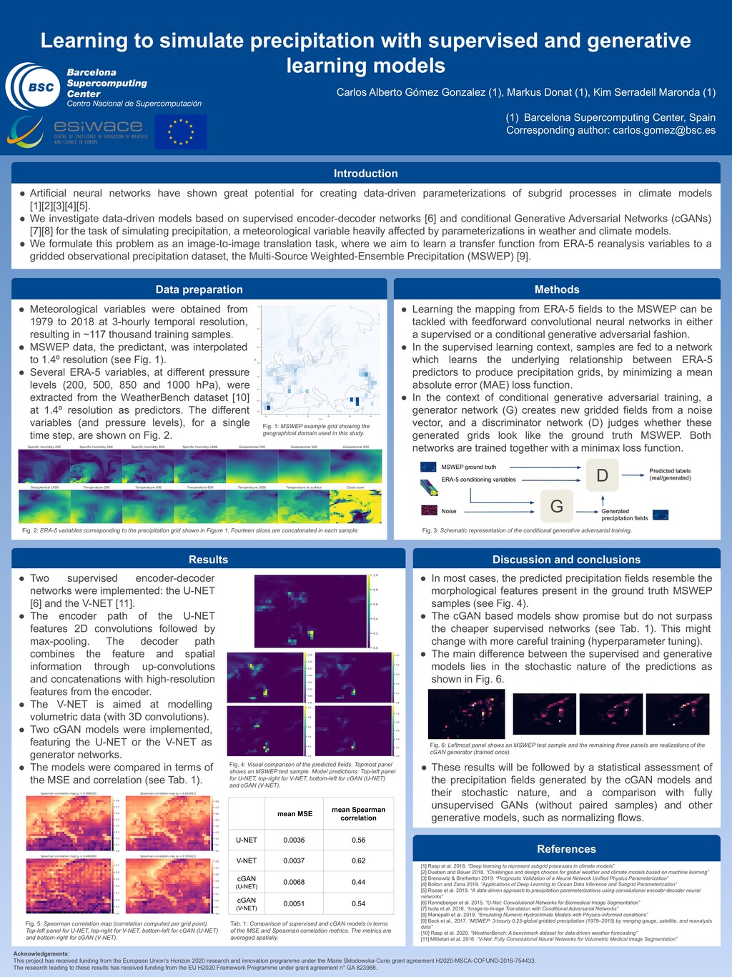
1. Learning to simulate precipitation with supervised and generative learning models Carlos Alberto Gómez Gonzalez (1), Markus Donat (1), Kim Serradell Maronda (1) (1) Barcelona Supercomputing Center, Spain Corresponding author: carlos.gomez@bsc.es Discussion and conclusions • Meteorological variables were obtained from 1979 to 2018 at 3-hourly temporal resolution, resulting in ~117 thousand training samples. • MSWEP data, the predictant, was interpolated to 1.4º resolution (see Fig. 1). • Several ERA-5 variables, at different pressure levels (200, 500, 850 and 1000 hPa), were extracted from the WeatherBench dataset [10] at 1.4º resolution as predictors. The different variables (and pressure levels), for a single time step, are shown on Fig. 2. Data preparation • Artificial neural networks have shown great potential for creating data-driven parameterizations of subgrid processes in climate models [1][2][3][4][5]. • We investigate data-driven models based on supervised encoder-decoder networks [6] and conditional Generative Adversarial Networks (cGANs) [7][8] for the task of simulating precipitation, a meteorological variable heavily affected by parameterizations in weather and climate models. • We formulate this problem as an image-to-image translation task, where we aim to learn a transfer function from ERA-5 reanalysis variables to a gridded observational precipitation dataset, the Multi-Source Weighted-Ensemble Precipitation (MSWEP) [9]. Introduction Results [1] Rasp et al. 2018. “Deep learning to represent subgrid processes in climate models” [2] Dueben and Bauer 2018. “Challenges and design choices for global weather and climate models based on machine learning” [3] Brenowitz & Bretherton 2019. “Prognostic Validation of a Neural Network Unified Physics Parameterization” [4] Bolton and Zana 2019. “Applications of Deep Learning to Ocean Data Inference and Subgrid Parameterization” [5] Rozas et al. 2019. “A data-driven approach to precipitation parameterizations using convolutional encoder-decoder neural networks” [6] Ronneberger et al. 2015. “U-Net: Convolutional Networks for Biomedical Image Segmentation” [7] Isola et al. 2016. “Image-to-Image Translation with Conditional Adversarial Networks” [8] Manepalli et al. 2019. “Emulating Numeric Hydroclimate Models with Physics-Informed conditions” [9] Beck et al., 2017. “MSWEP: 3-hourly 0.25◦global gridded precipitation (1979–2015) by merging gauge, satellite, and reanalysis data” [10] Rasp et al. 2020. “WeatherBench: A benchmark dataset for data-driven weather forecasting” [11] Millietari et al. 2016. “V-Net: Fully Convolutional Neural Networks for Volumetric Medical Image Segmentation” References • Two supervised encoder-decoder networks were implemented: the U-NET [6] and the V-NET [11]. • The encoder path of the U-NET features 2D convolutions followed by max-pooling. The decoder path combines the feature and spatial information through up-convolutions and concatenations with high-resolution features from the encoder. • The V-NET is aimed at modelling volumetric data (with 3D convolutions). • Two cGAN models were implemented, featuring the U-NET or the V-NET as generator networks. • The models were compared in terms of the MSE and correlation (see Tab. 1). • In most cases, the predicted precipitation fields resemble the morphological features present in the ground truth MSWEP samples (see Fig. 4). • The cGAN based models show promise but do not surpass the cheaper supervised networks (see Tab. 1). This might change with more careful training (hyperparameter tuning). • The main difference between the supervised and generative models lies in the stochastic nature of the predictions as shown in Fig. 6. • These results will be followed by a statistical assessment of the precipitation fields generated by the cGAN models and their stochastic nature, and a comparison with fully unsupervised GANs (without paired samples) and other generative models, such as normalizing flows. • Learning the mapping from ERA-5 fields to the MSWEP can be tackled with feedforward convolutional neural networks in either a supervised or a conditional generative adversarial fashion. • In the supervised learning context, samples are fed to a network which learns the underlying relationship between ERA-5 predictors to produce precipitation grids, by minimizing a mean absolute error (MAE) loss function. • In the context of conditional generative adversarial training, a generator network (G) creates new gridded fields from a noise vector, and a discriminator network (D) judges whether these generated grids look like the ground truth MSWEP. Both networks are trained together with a minimax loss function. Methods Fig. 1: MSWEP example grid showing the geographical domain used in this study. Fig. 2: ERA-5 variables corresponding to the precipitation grid shown in Figure 1. Fourteen slices are concatenated in each sample. mean MSE mean Spearman correlation U-NET 0.0036 0.56 V-NET 0.0037 0.62 cGAN (U-NET) 0.0068 0.44 cGAN (V-NET) 0.0051 0.54 Fig. 3: Schematic representation of the conditional generative adversarial training. D G MSWEP ground truth ERA-5 conditioning variables Noise Generated precipitation fields Predicted labels (real/generated) Tab. 1: Comparison of supervised and cGAN models in terms of the MSE and Spearman correlation metrics. The metrics are averaged spatially. Fig. 5: Spearman correlation map (correlation computed per grid point). Top-left panel for U-NET, top-right for V-NET, bottom-left for cGAN (U-NET) and bottom-right for cGAN (V-NET). Fig. 4: Visual comparison of the predicted fields. Topmost panel shows an MSWEP test sample. Model predictions: Top-left panel for U-NET, top-right for V-NET, bottom-left for cGAN (U-NET) and cGAN (V-NET). Fig. 6: Leftmost panel shows an MSWEP test sample and the remaining three panels are realizations of the cGAN generator (trained once). Acknowledgements: This project has received funding from the European Union’s Horizon 2020 research and innovation programme under the Marie Skłodowska-Curie grant agreement H2020-MSCA-COFUND-2016-754433. The research leading to these results has received funding from the EU H2020 Framework Programme under grant agreement n° GA 823988.