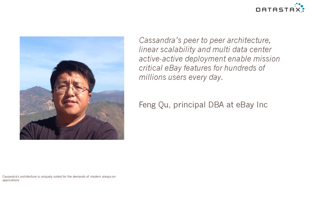
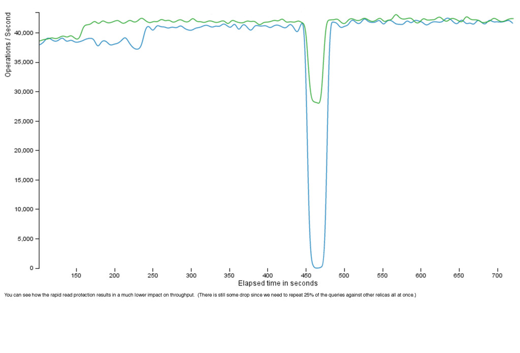
center active-active deployment enable mission critical eBay features for hundreds of millions users every day. Feng Qu, principal DBA at eBay Inc Cassandra’s architecture is uniquely suited for the demands of modern always-on applications
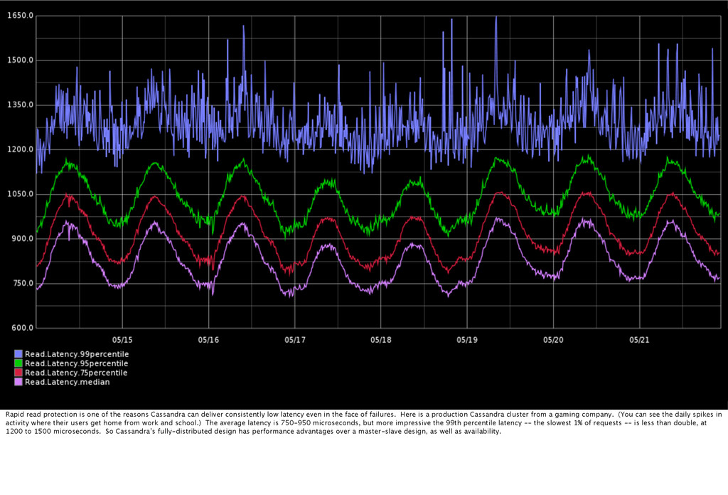
deliver consistently low latency even in the face of failures. Here is a production Cassandra cluster from a gaming company. (You can see the daily spikes in activity where their users get home from work and school.) The average latency is 750-950 microseconds, but more impressive the 99th percentile latency -- the slowest 1% of requests -- is less than double, at 1200 to 1500 microseconds. So Cassandra’s fully-distributed design has performance advantages over a master-slave design, as well as availability.
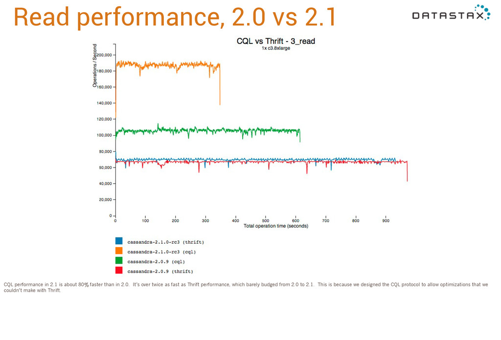
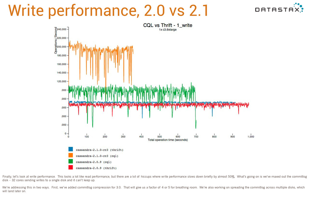
about 80% faster than in 2.0. It’s over twice as fast as Thrift performance, which barely budged from 2.0 to 2.1. This is because we designed the CQL protocol to allow optimizations that we couldn’t make with Thrift.
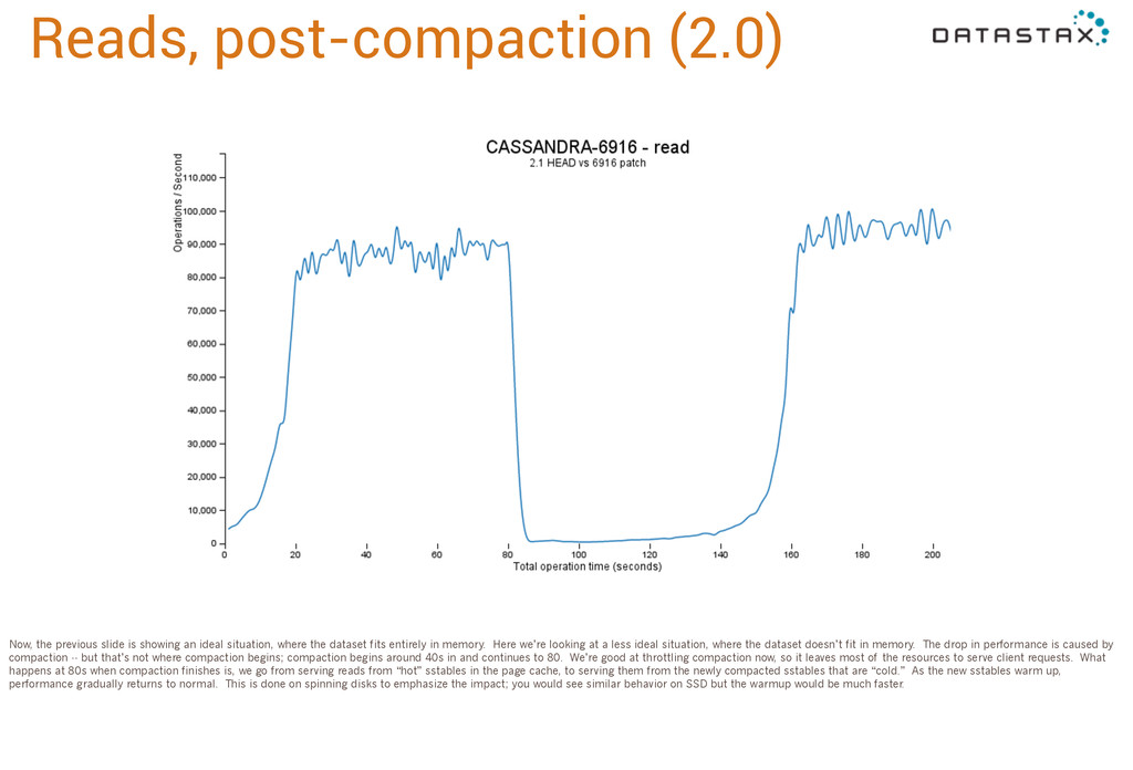
ideal situation, where the dataset fits entirely in memory. Here we’re looking at a less ideal situation, where the dataset doesn’t fit in memory. The drop in performance is caused by compaction -- but that’s not where compaction begins; compaction begins around 40s in and continues to 80. We’re good at throttling compaction now, so it leaves most of the resources to serve client requests. What happens at 80s when compaction finishes is, we go from serving reads from “hot” sstables in the page cache, to serving them from the newly compacted sstables that are “cold.” As the new sstables warm up, performance gradually returns to normal. This is done on spinning disks to emphasize the impact; you would see similar behavior on SSD but the warmup would be much faster.
the new sstables immediately. As soon as we finish compacting a block of partitions, we’ll start serving reads from the new, compacted sstable. So when we finish we just promote the new sstable to permanent and delete the old ones. There is no performance “cliff” because we’ve been gradually warming up the new sstable the entire time.
performance. This looks a lot like read performance, but there are a lot of hiccups where write performance slows down briefly by almost 50%. What’s going on is we’ve maxed out the commitlog disk -- 32 cores sending writes to a single disk and it can’t keep up. We’re addressing this in two ways. First, we’ve added commitlog compression for 3.0. That will give us a factor of 4 or 5 for breathing room. We’re also working on spreading the commitlog across multiple disks, which will land later on.
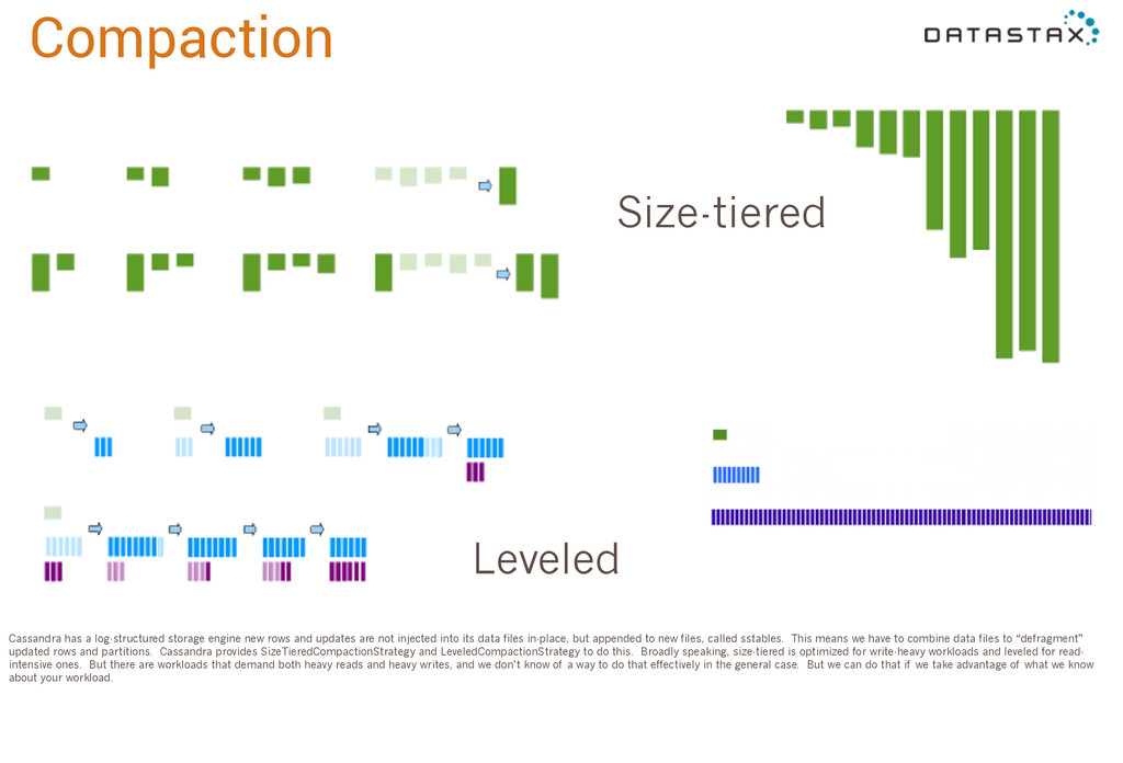
rows and updates are not injected into its data files in-place, but appended to new files, called sstables. This means we have to combine data files to “defragment” updated rows and partitions. Cassandra provides SizeTieredCompactionStrategy and LeveledCompactionStrategy to do this. Broadly speaking, size-tiered is optimized for write-heavy workloads and leveled for read- intensive ones. But there are workloads that demand both heavy reads and heavy writes, and we don’t know of a way to do that effectively in the general case. But we can do that if we take advantage of what we know about your workload.
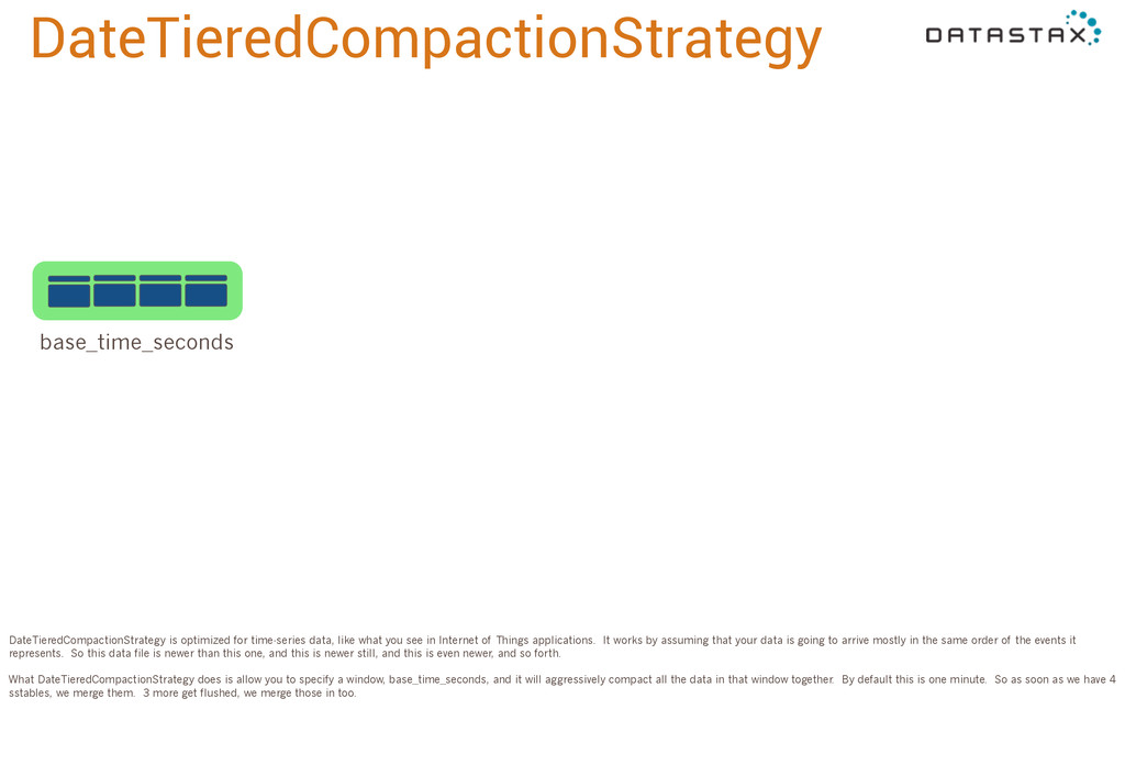
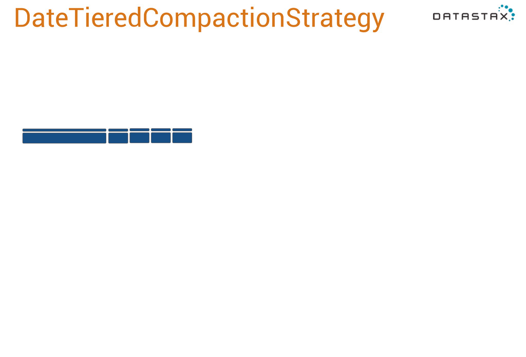
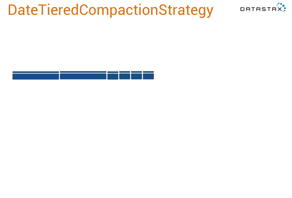
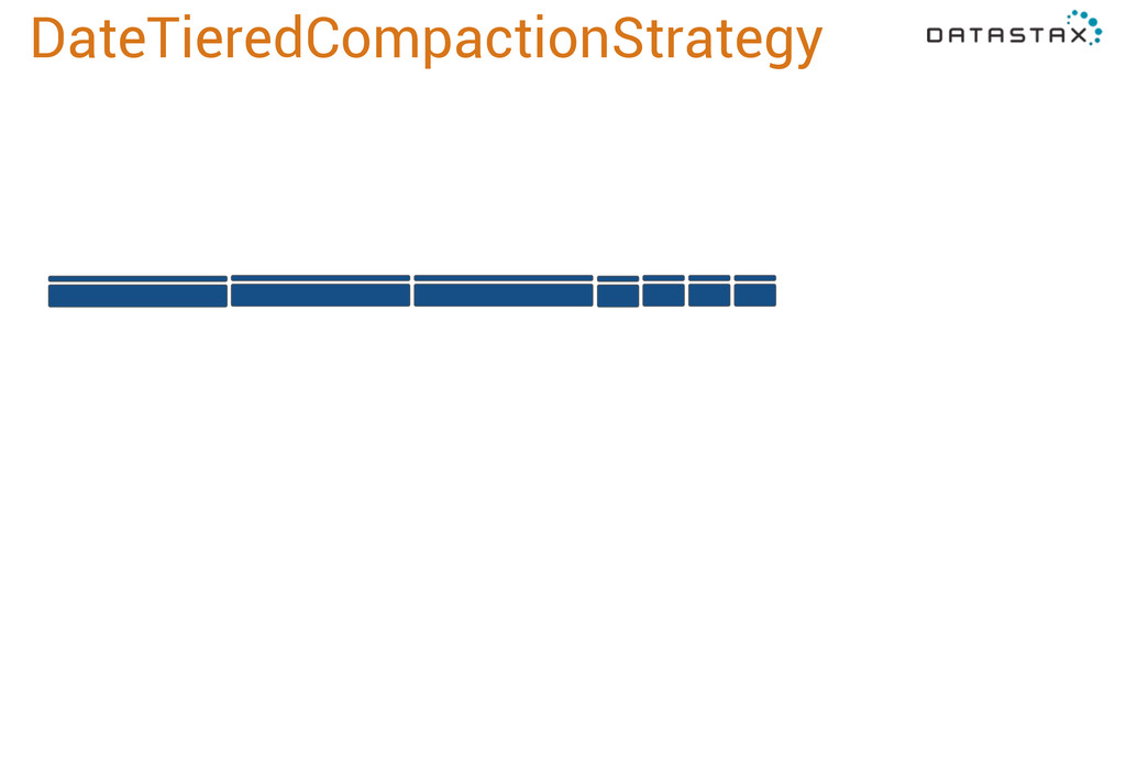
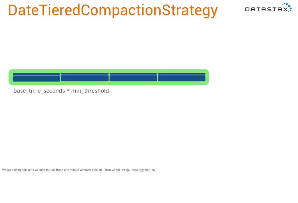
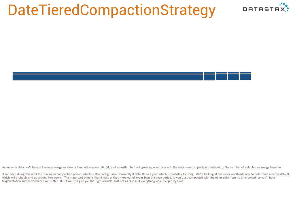
you see in Internet of Things applications. It works by assuming that your data is going to arrive mostly in the same order of the events it represents. So this data file is newer than this one, and this is newer still, and this is even newer, and so forth. What DateTieredCompactionStrategy does is allow you to specify a window, base_time_seconds, and it will aggressively compact all the data in that window together. By default this is one minute. So as soon as we have 4 sstables, we merge them. 3 more get flushed, we merge those in too.
merge window, a 4 minute window, 16, 64, and so forth. So it will grow exponentially with the minimum compaction threshold, or the number of sstables we merge together. It will keep doing this until the maximum compaction period, which is also configurable. Currently it defaults to a year, which is probably too long. We’re looking at customer workloads now to determine a better default, which will probably end up around two weeks. The important thing is that if data arrives more out of order than this max period, it won’t get compacted with the other data from its time period, so you’ll have fragmentation and performance will suffer. But it will still give you the right results! Just not as fast as if everything were merged by time.
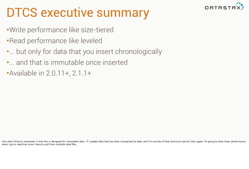
leveled •... but only for data that you insert chronologically •... and that is immutable once inserted •Available in 2.0.11+, 2.1.1+ One other thing to remember is that this is designed for immutable data. If I update data that has been compacted by date, and I’m outside of that maximum period, then again I’m going to have lower performance when I go to read that since I have to pull from multiple data files.
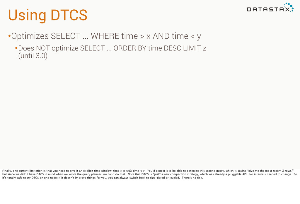
time < y •Does NOT optimize SELECT ... ORDER BY time DESC LIMIT z (until 3.0) Finally, one current limitation is that you need to give it an explicit time window: time > x AND time < y. You’d expect it to be able to optimize this second query, which is saying “give me the most recent Z rows,” but since we didn’t have DTCS in mind when we wrote the query planner, we can’t do that. Note that DTCS is *just* a new compaction strategy, which was already a pluggable API. No internals needed to change. So it’s totally safe to try DTCS on one node; if it doesn’t improve things for you, you can always switch back to size-tiered or leveled. There’s no risk.
False | pmcfadin | 2011-06-20 ... | Patrick McFadin INSERT INTO users (username, name, email, password, created_date) VALUES ('pmcfadin', 'Patrick McFadin', ['[email protected]'], 'ba27e03fd9...', '2011-06-20 13:50:00') IF NOT EXISTS; [applied] ----------- True INSERT INTO users (username, name, email, password, created_date) VALUES ('pmcfadin', 'Patrick McFadin', ['[email protected]'], 'ea24e13ad9...', '2011-06-20 13:50:01') IF NOT EXISTS; As you know, lightweight transactions [LWT[ allow us to perform ACID operations within a single partition by adding an “IF” clause with a condition to check before applying an INSERT or UPDATE.
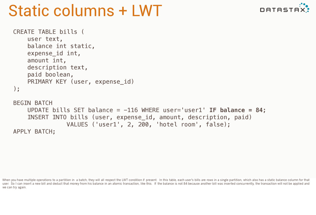
int static, expense_id int, amount int, description text, paid boolean, PRIMARY KEY (user, expense_id) ); We’ve added some new features that make LWT more interesting. Static columns is one of those. “Static” means that the column is shared across all the rows in a partition, just like a Java static field is shared across all the instances of a class.
balance int static, expense_id int, amount int, description text, paid boolean, PRIMARY KEY (user, expense_id) ); BEGIN BATCH UPDATE bills SET balance = -116 WHERE user='user1' IF balance = 84; INSERT INTO bills (user, expense_id, amount, description, paid) VALUES ('user1', 2, 200, 'hotel room', false); APPLY BATCH; When you have multiple operations to a partition in a batch, they will all respect the LWT condition if present. In this table, each user’s bills are rows in a single partition, which also has a static balance column for that user. So I can insert a new bill and deduct that money from his balance in an atomic transaction, like this. If the balance is not 84 because another bill was inserted concurrently, the transaction will not be applied and we can try again.
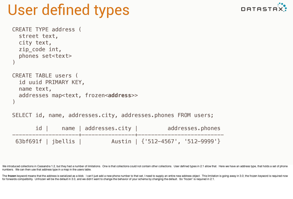
text, zip_code int, phones set<text> ) CREATE TABLE users ( id uuid PRIMARY KEY, name text, addresses map<text, frozen<address>> ) SELECT id, name, addresses.city, addresses.phones FROM users; id | name | addresses.city | addresses.phones --------------------+----------------+-------------------------- 63bf691f | jbellis | Austin | {'512-4567', '512-9999'} We introduced collections in Cassandra 1.2, but they had a number of limitations. One is that collections could not contain other collections. User defined types in 2.1 allow that. Here we have an address type, that holds a set of phone numbers. We can then use that address type in a map in the users table. The frozen keyword means that the address is serialized as a blob. I can’t just add a new phone number to that set, I need to supply an entire new address object. This limitation is going away in 3.0; the frozen keyword is required now for forwards compatibility. Unfrozen will be the default in 3.0, and we didn’t want to change the behavior of your schema by changing the default. So “frozen” is required in 2.1.
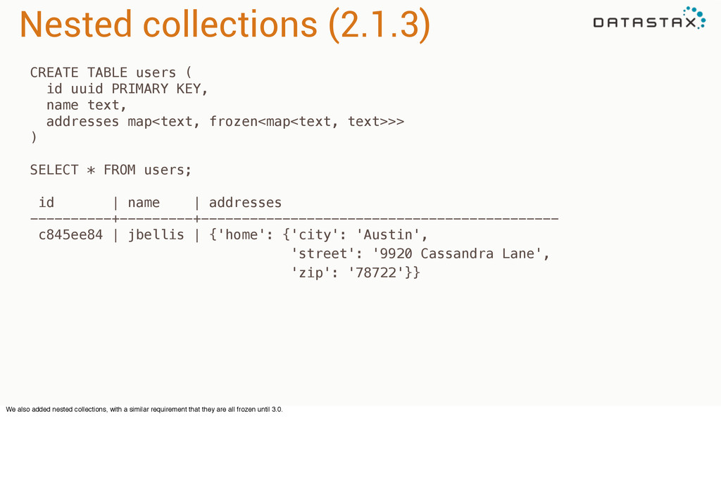
KEY, name text, addresses map<text, frozen<map<text, text>>> ) SELECT * FROM users; id | name | addresses ----------+---------+-------------------------------------------- c845ee84 | jbellis | {'home': {'city': 'Austin', 'street': '9920 Cassandra Lane', 'zip': '78722'}} We also added nested collections, with a similar requirement that they are all frozen until 3.0.
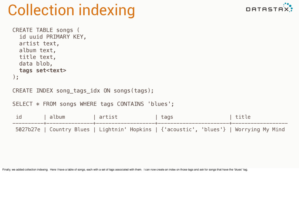
artist text, album text, title text, data blob, tags set<text> ); CREATE INDEX song_tags_idx ON songs(tags); SELECT * FROM songs WHERE tags CONTAINS 'blues'; id | album | artist | tags | title ----------+---------------+-------------------+-----------------------+------------------ 5027b27e | Country Blues | Lightnin' Hopkins | {'acoustic', 'blues'} | Worrying My Mind Finally, we added collection indexing. Here I have a table of songs, each with a set of tags associated with them. I can now create an index on those tags and ask for songs that have the “blues” tag.
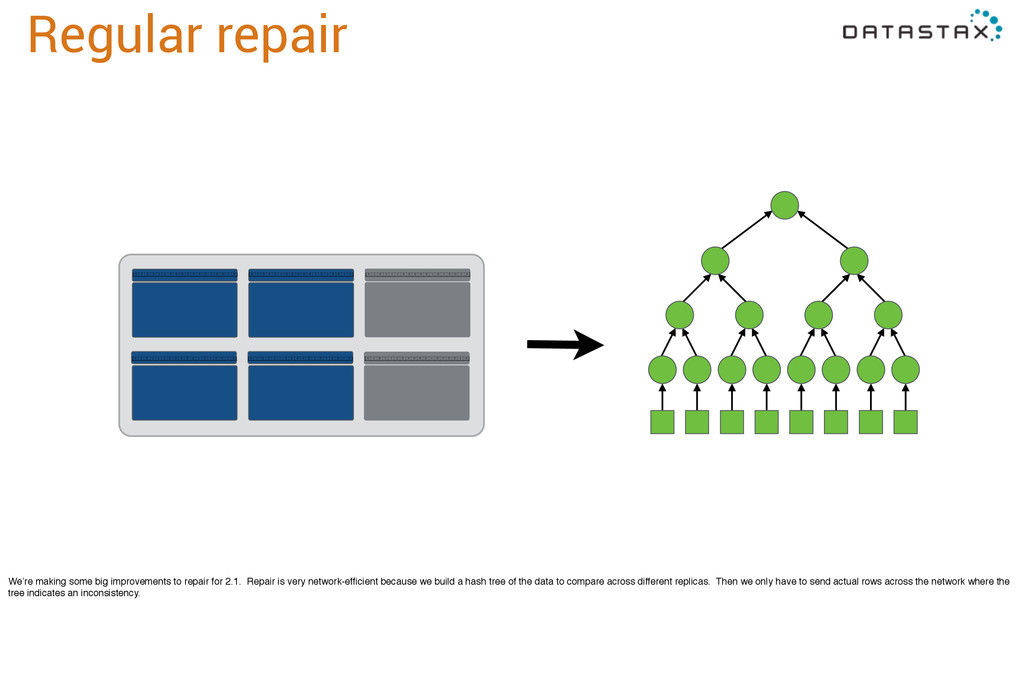
2.1. Repair is very network-efficient because we build a hash tree of the data to compare across different replicas. Then we only have to send actual rows across the network where the tree indicates an inconsistency.
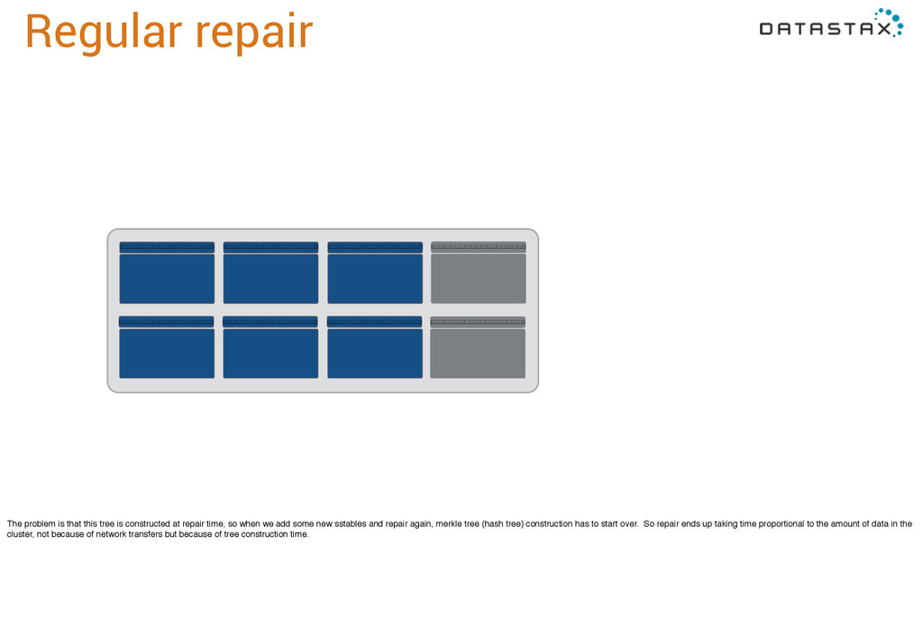
at repair time, so when we add some new sstables and repair again, merkle tree (hash tree) construction has to start over. So repair ends up taking time proportional to the amount of data in the cluster, not because of network transfers but because of tree construction time.
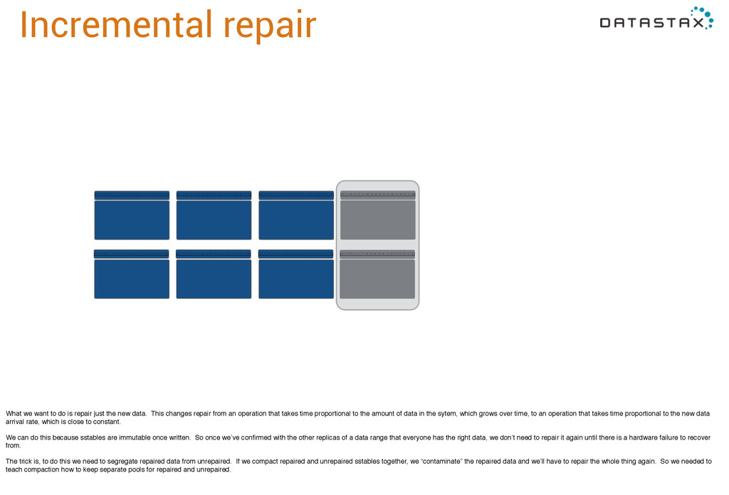
the new data. This changes repair from an operation that takes time proportional to the amount of data in the sytem, which grows over time, to an operation that takes time proportional to the new data arrival rate, which is close to constant. We can do this because sstables are immutable once written. So once we’ve confirmed with the other replicas of a data range that everyone has the right data, we don’t need to repair it again until there is a hardware failure to recover from. The trick is, to do this we need to segregate repaired data from unrepaired. If we compact repaired and unrepaired sstables together, we “contaminate” the repaired data and we’ll have to repair the whole thing again. So we needed to teach compaction how to keep separate pools for repaired and unrepaired.
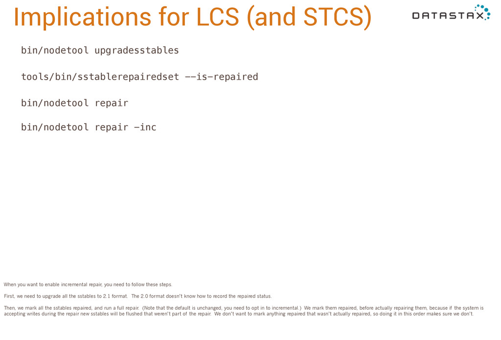
repair bin/nodetool repair -inc When you want to enable incremental repair, you need to follow these steps. First, we need to upgrade all the sstables to 2.1 format. The 2.0 format doesn’t know how to record the repaired status. Then, we mark all the sstables repaired, and run a full repair. (Note that the default is unchanged, you need to opt in to incremental.) We mark them repaired, before actually repairing them, because if the system is accepting writes during the repair new sstables will be flushed that weren’t part of the repair. We don’t want to mark anything repaired that wasn’t actually repaired, so doing it in this order makes sure we don’t.
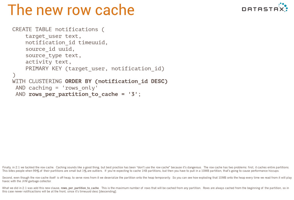
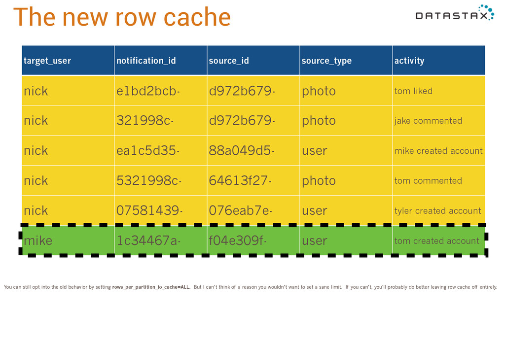
notification_id timeuuid, source_id uuid, source_type text, activity text, PRIMARY KEY (target_user, notification_id) ) WITH CLUSTERING ORDER BY (notification_id DESC) AND caching = 'rows_only' AND rows_per_partition_to_cache = '3'; Finally, in 2.1 we tackled the row cache. Caching sounds like a good thing, but best practice has been “don’t use the row cache” because it’s dangerous. The row cache has two problems: first, it caches entire partitions. This bites people when 99% of their partitions are small but 1% are outliers. If you’re expecting to cache 1KB partitions, but then you have to pull in a 10MB partition, that’s going to cause performance hiccups. Second, even though the row cache itself is off-heap, to serve rows from it we deserialize the partition onto the heap temporarily. So you can see how exploding that 10MB onto the heap every time we read from it will play havoc with the JVM garbage collector. What we did in 2.1 was add this new clause, rows_per_partition_to_cache. This is the maximum number of rows that will be cached from any partition. Rows are always cached from the beginning of the partition, so in this case newer notificactions will be at the front, since it’s timeuuid desc [descending].
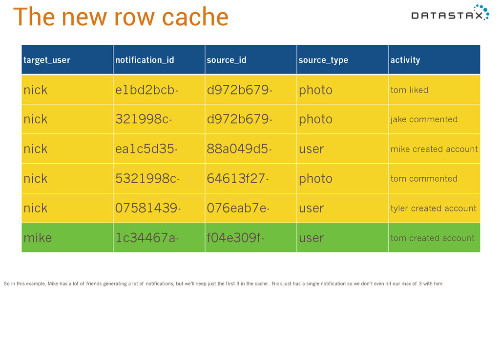
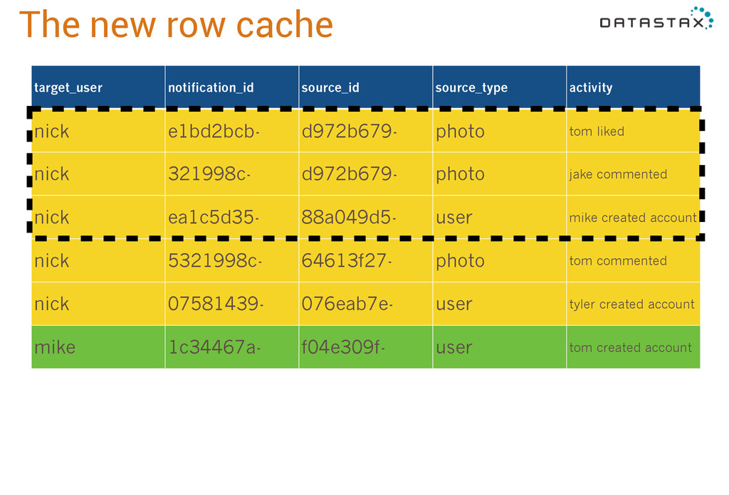
e1bd2bcb- d972b679- photo tom liked nick 321998c- d972b679- photo jake commented nick ea1c5d35- 88a049d5- user mike created account nick 5321998c- 64613f27- photo tom commented nick 07581439- 076eab7e- user tyler created account mike 1c34467a- f04e309f- user tom created account So in this example, Mike has a lot of friends generating a lot of notifications, but we’ll keep just the first 3 in the cache. Nick just has a single notification so we don’t even hit our max of 3 with him.
liked nick 321998c- d972b679- photo jake commented nick ea1c5d35- 88a049d5- user mike created account nick 5321998c- 64613f27- photo tom commented nick 07581439- 076eab7e- user tyler created account mike 1c34467a- f04e309f- user tom created account The new row cache
e1bd2bcb- d972b679- photo tom liked nick 321998c- d972b679- photo jake commented nick ea1c5d35- 88a049d5- user mike created account nick 5321998c- 64613f27- photo tom commented nick 07581439- 076eab7e- user tyler created account mike 1c34467a- f04e309f- user tom created account You can still opt into the old behavior by setting rows_per_partition_to_cache=ALL. But I can’t think of a reason you wouldn’t want to set a sane limit. If you can’t, you’ll probably do better leaving row cache off entirely.
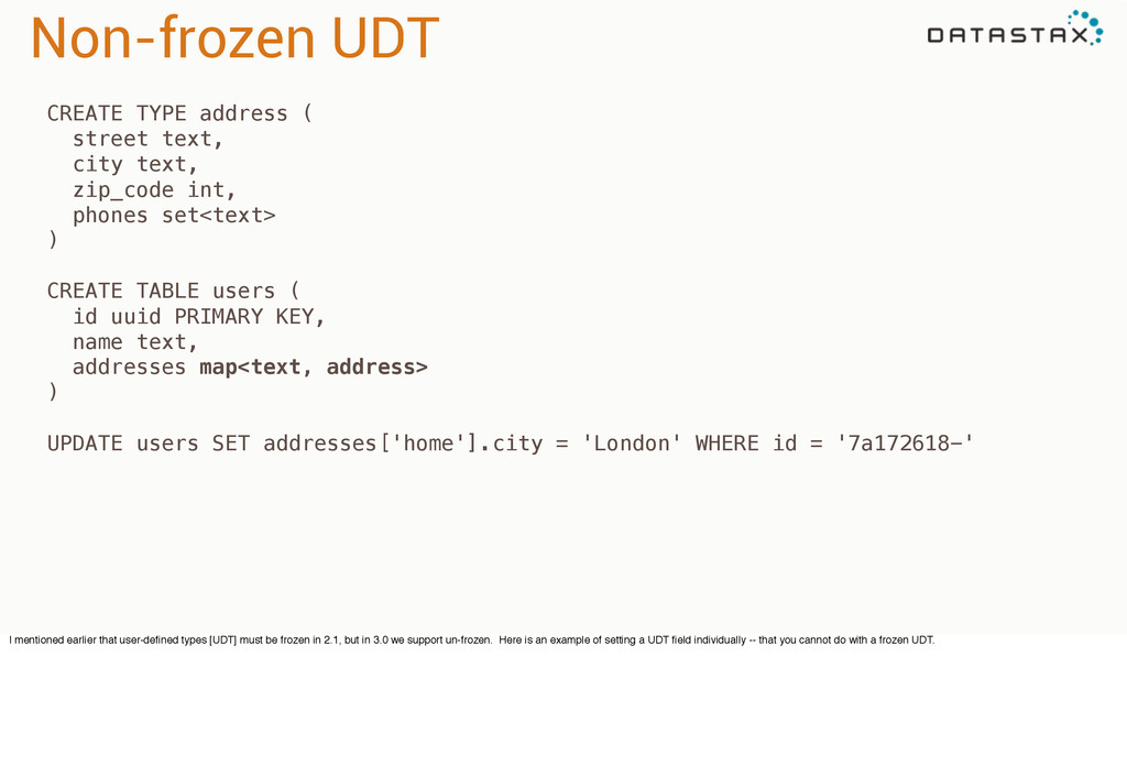
zip_code int, phones set<text> ) CREATE TABLE users ( id uuid PRIMARY KEY, name text, addresses map<text, address> ) UPDATE users SET addresses['home'].city = 'London' WHERE id = '7a172618-' I mentioned earlier that user-defined types [UDT] must be frozen in 2.1, but in 3.0 we support un-frozen. Here is an example of setting a UDT field individually -- that you cannot do with a frozen UDT.
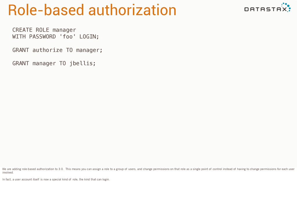
authorize TO manager; GRANT manager TO jbellis; We are adding role-based authorization to 3.0. This means you can assign a role to a group of users, and change permissions on that role as a single point of control instead of having to change permissions for each user involved. In fact, a user account itself is now a special kind of role, the kind that can login.
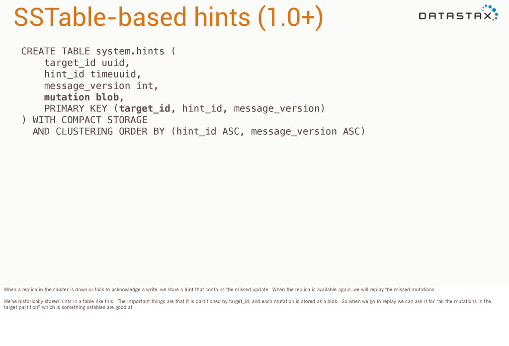
timeuuid, message_version int, mutation blob, PRIMARY KEY (target_id, hint_id, message_version) ) WITH COMPACT STORAGE AND CLUSTERING ORDER BY (hint_id ASC, message_version ASC) When a replica in the cluster is down or fails to acknowledge a write, we store a hint that contains the missed update. When the replica is available again, we will replay the missed mutations. We’ve historically stored hints in a table like this. The important things are that it is partitioned by target_id, and each mutation is stored as a blob. So when we go to replay we can ask it for “all the mutations in the target partition” which is something sstables are good at.
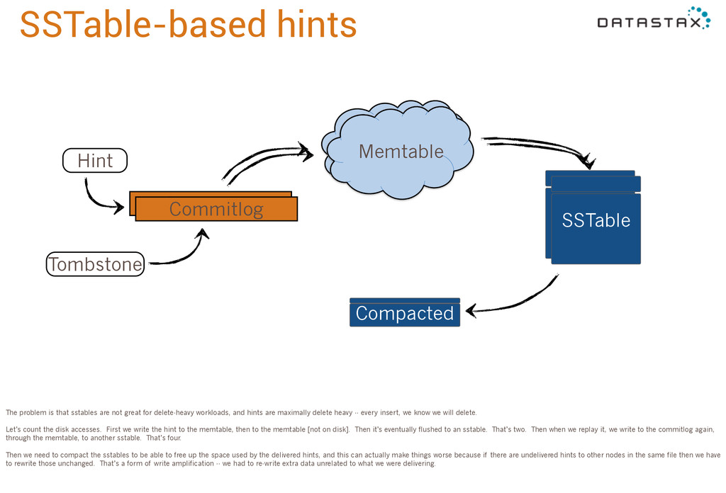
Compacted The problem is that sstables are not great for delete-heavy workloads, and hints are maximally delete heavy -- every insert, we know we will delete. Let’s count the disk accesses. First we write the hint to the memtable, then to the memtable [not on disk]. Then it’s eventually flushed to an sstable. That’s two. Then when we replay it, we write to the commitlog again, through the memtable, to another sstable. That’s four. Then we need to compact the sstables to be able to free up the space used by the delivered hints, and this can actually make things worse because if there are undelivered hints to other nodes in the same file then we have to rewrite those unchanged. That’s a form of write amplification -- we had to re-write extra data unrelated to what we were delivering.
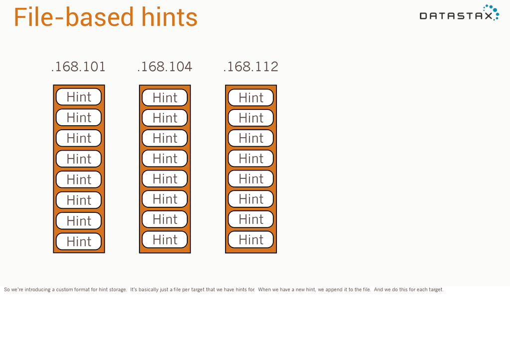
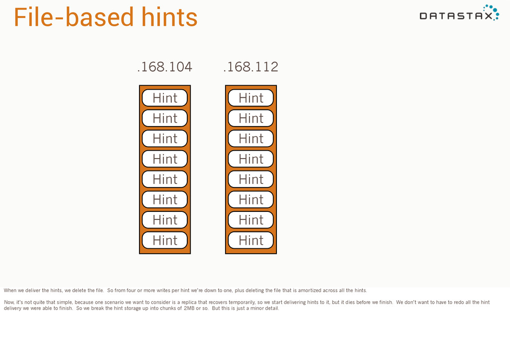
Hint .168.104 Hint Hint Hint Hint Hint Hint Hint Hint .168.112 Hint Hint Hint Hint Hint Hint Hint Hint So we’re introducing a custom format for hint storage. It’s basically just a file per target that we have hints for. When we have a new hint, we append it to the file. And we do this for each target.
Hint .168.112 Hint Hint Hint Hint Hint Hint Hint Hint When we deliver the hints, we delete the file. So from four or more writes per hint we’re down to one, plus deleting the file that is amortized across all the hints. Now, it’s not quite that simple, because one scenario we want to consider is a replica that recovers temporarily, so we start delivering hints to it, but it dies before we finish. We don’t want to have to redo all the hint delivery we were able to finish. So we break the hint storage up into chunks of 2MB or so. But this is just a minor detail.
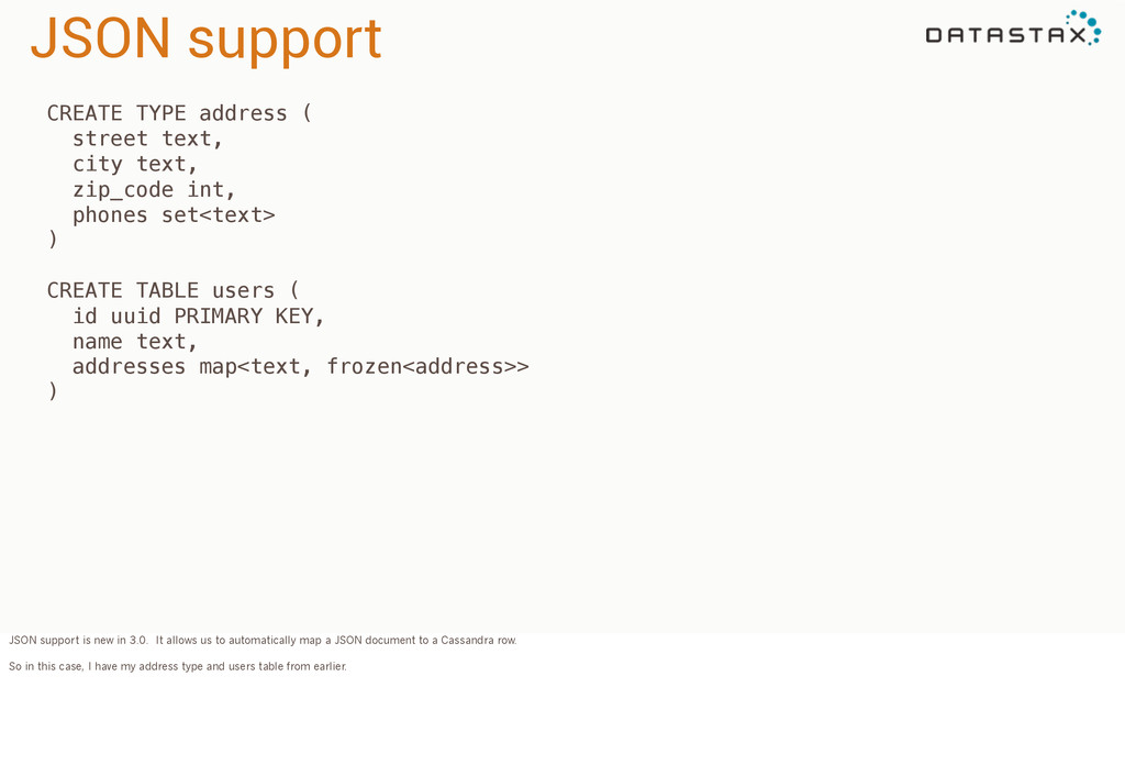
zip_code int, phones set<text> ) CREATE TABLE users ( id uuid PRIMARY KEY, name text, addresses map<text, frozen<address>> ) JSON support is new in 3.0. It allows us to automatically map a JSON document to a Cassandra row. So in this case, I have my address type and users table from earlier.
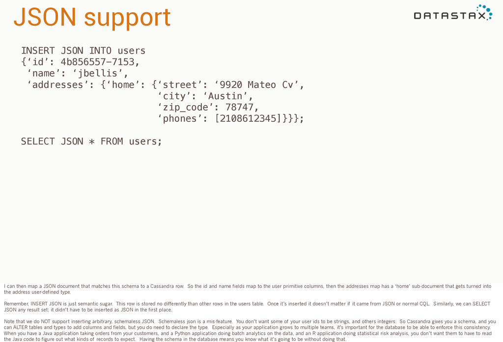
‘addresses’: {‘home’: {‘street’: ‘9920 Mateo Cv’, ‘city’: ‘Austin’, ‘zip_code’: 78747, ‘phones’: [2108612345]}}}; SELECT JSON * FROM users; I can then map a JSON document that matches this schema to a Cassandra row. So the id and name fields map to the user primitive columns, then the addresses map has a ‘home’ sub-document that gets turned into the address user-defined type. Remember, INSERT JSON is just semantic sugar. This row is stored no differently than other rows in the users table. Once it’s inserted it doesn’t matter if it came from JSON or normal CQL. Similarly, we can SELECT JSON any result set; it didn’t have to be inserted as JSON in the first place. Note that we do NOT support inserting arbitrary, schemaless JSON. Schemaless json is a mis-feature. You don’t want some of your user ids to be strings, and others integers. So Cassandra gives you a schema, and you can ALTER tables and types to add columns and fields, but you do need to declare the type. Especially as your application grows to multiple teams, it’s important for the database to be able to enforce this consistency. When you have a Java application taking orders from your customers, and a Python application doing batch analytics on the data, and an R application doing statistical risk analysis, you don’t want them to have to read the Java code to figure out what kinds of records to expect. Having the schema in the database means you know what it’s going to be without doing that.
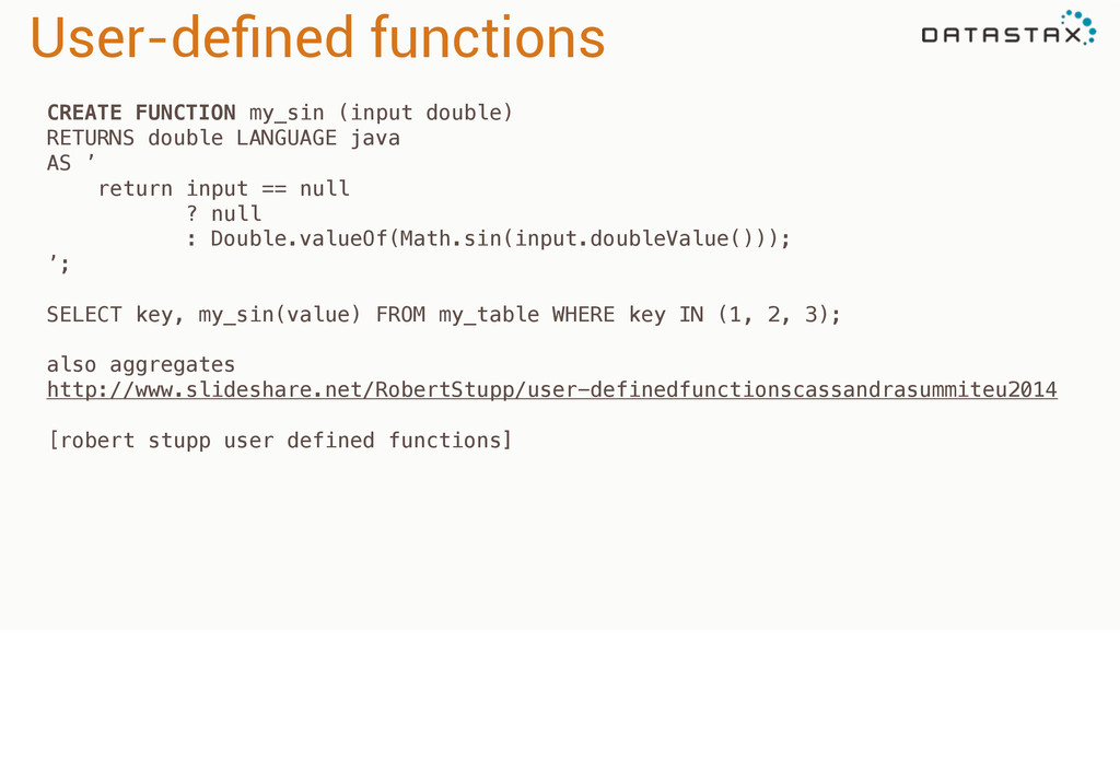
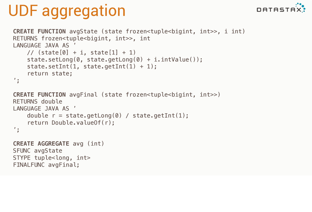
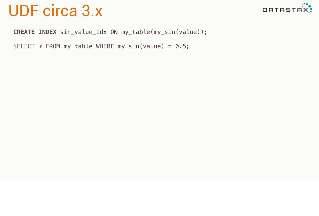
java AS ’ return input == null ? null : Double.valueOf(Math.sin(input.doubleValue())); ’; SELECT key, my_sin(value) FROM my_table WHERE key IN (1, 2, 3); also aggregates http://www.slideshare.net/RobertStupp/user-definedfunctionscassandrasummiteu2014 [robert stupp user defined functions]
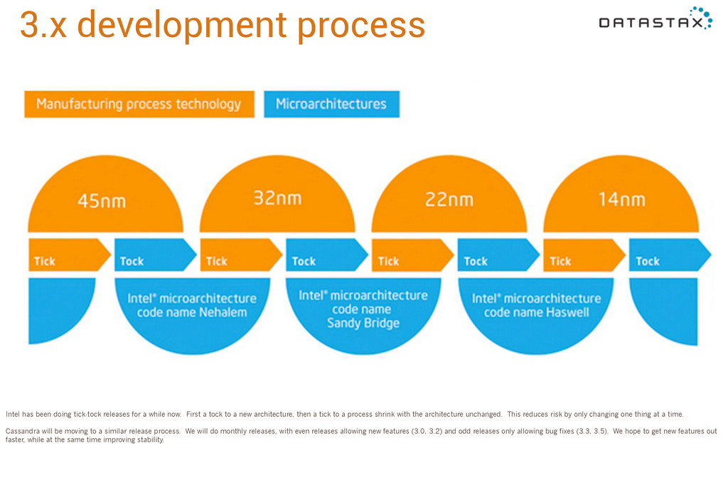
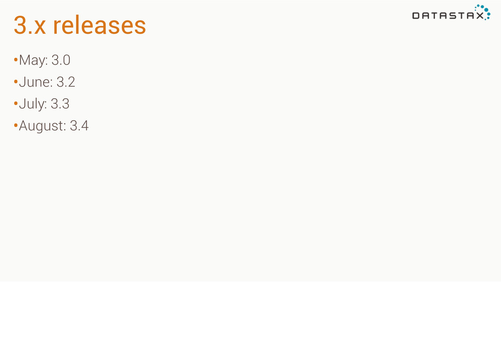
a while now. First a tock to a new architecture, then a tick to a process shrink with the architecture unchanged. This reduces risk by only changing one thing at a time. Cassandra will be moving to a similar release process. We will do monthly releases, with even releases allowing new features (3.0, 3.2) and odd releases only allowing bug fixes (3.3, 3.5). We hope to get new features out faster, while at the same time improving stability.
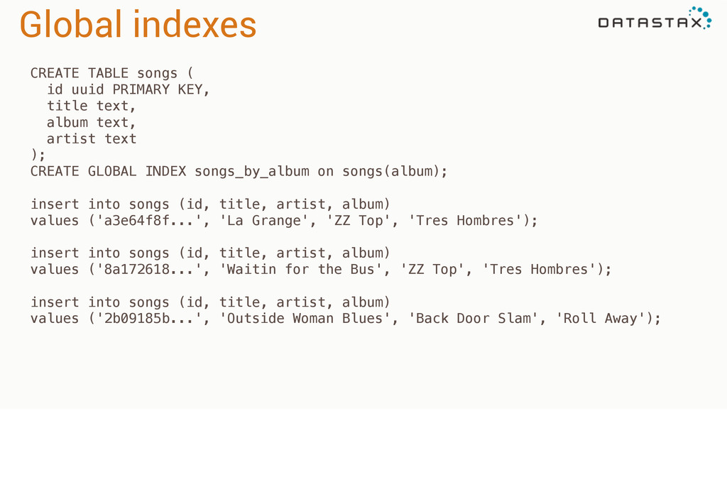
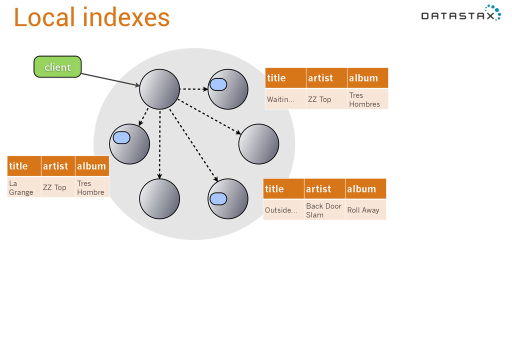
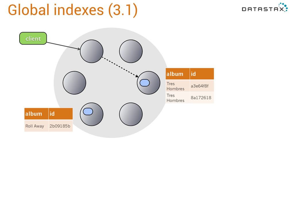
title text, album text, artist text ); CREATE GLOBAL INDEX songs_by_album on songs(album); insert into songs (id, title, artist, album) values ('a3e64f8f...', 'La Grange', 'ZZ Top', 'Tres Hombres'); insert into songs (id, title, artist, album) values ('8a172618...', 'Waitin for the Bus', 'ZZ Top', 'Tres Hombres'); insert into songs (id, title, artist, album) values ('2b09185b...', 'Outside Woman Blues', 'Back Door Slam', 'Roll Away');
![Lightweight transactions [applied] | username | created_date | name -----------+----------+----------------+----------------](https://files.speakerdeck.com/presentations/ed2c8cb5b7d3477cb9e9bd707091dfee/slide_22.jpg)