Naive Bayes ACM SIGKDD

Session 4: Naive Bayes Algorithms, Advanced Machine Learning with Python, ACM SIGKDD, Austin TX

Transcript

1. Naive Bayes Algorithms Advanced Machine Learning with Python Session 4, ACM SIGKDD Christine Doig Senior Data Scientist
2. Presenter Bio Christine Doig is a Senior Data Scientist at Continuum Analytics, where she worked on MEMEX, a DARPA- funded project helping stop human trafficking. She has 5+ years of experience in analytics, operations research, and machine learning in a variety of industries, including energy, manufacturing, and banking. Christine holds a M.S. in Industrial Engineering from the Polytechnic University of Catalonia in Barcelona. She is an open source advocate and has spoken at many conferences, including PyData, EuroPython, SciPy and PyCon. Christine Doig
 Senior Data Scientist Continuum Analytics @ch_doig
3. Previous talks • Topic Modeling, Machine Learning with Python, ACM SIGKDD’15 • Scale your data, not your process. Welcome to the Blaze ecosystem! , EuroPython’15 • Reproducible Multilanguage Data Science with conda, PyData Dallas’15 • Building Python Data Applications with Blaze and Bokeh, SciPy’15 • Navigating the Data Science Python Ecosystem, PyConES’15 • The State of Python for Data Science, PySS’15 • Beginner’s Guide to Machine Learning Competitions, PyTexas’15 Christine Doig
 Senior Data Scientist Continuum Analytics @ch_doig
4. INTRODUCTION
6. 6 Machine Learning Supervised Unsupervised Classification Regression Clustering labeled not labeled categorical quatitative variable to predict (Y)
7. 7 Classification Discrete-valued inputs (X) Continuous inputs (X) MultinomialNB BernouilliNB GaussianNB Naive Bayes Algorithms occurance counts binary/boolean features
8. Naive Bayes Algorithms • Probability Review – Joint distribution, Conditional probability – Bayes Theorem, Naive Bayes classifiers • Multinomial NB • Bernouilli NB • Gaussian NB
9. PROBABILITY CONCEPTS REVIEW
10. Data Feature X1 Feature X2 Feature X3 Label Y instance 1 instance 2 instance 3 instance 4
11. Data Feature X1 Feature X2 Feature X3 Label Y instance 1 instance 2 instance 3 instance 4 X Y
12. Data - Simple Example Rainy Ice cream Traffic jam Label Y day 1 0 1 1 happy day 2 0 1 1 happy day 3 1 0 1 sad day 4 0 0 0 happy Example: Variable Y to predict is categorical and X are discrete
13. Data - Simple Example Rainy Ice cream Traffic jam Label Y day 1 0 1 1 happy day 2 0 1 1 happy day 3 1 0 1 sad day 4 0 0 0 happy day 5 0 0 1 sad day 6 0 1 1 sad day 7 1 1 0 sad day 8 0 1 1 happy day 9 0 0 0 happy day 10 1 0 1 sad Rainy Ice cream Traffic jam Label Y day 11 0 0 1 sad day 12 0 1 1 happy day 13 1 0 1 sad day 14 0 1 0 happy day 15 0 1 1 happy day 16 0 1 0 happy day 17 1 1 1 happy day 18 0 0 0 happy day 19 0 0 1 sad day 20 1 1 1 happy
14. Joint Probability Distribution In the study of probability, given at least two random variables X, Y, ..., that are defined on a probability space, the joint probability distribution for X, Y, ... is a probability distribution that gives the probability that each of X, Y, ... falls in any particular range or discrete set of values specified for that variable.
15. Rainy Ice cream Traffic jam Label Y day 1 0 1 1 happy day 2 0 1 1 happy day 3 1 0 1 sad day 4 0 0 0 happy Rainy Ice cream Probability 1 1 0.15 1 0 0.15 0 1 0.40 0 0 0.30 ? Count how many times we encounter each situation. Divide by total number of instances. Joint Probability Distribution
16. Conditional probability A conditional probability measures the probability of an event given that (by assumption, presumption, assertion or evidence) another event has occurred.
17. Computing probabilities Rainy Ice cream Probability 1 1 0.15 1 0 0.15 0 1 0.40 0 0 0.30 Pr(¬Rainy) = 0.70 Pr(Ice cream | Rainy) = 0.15 / 0.3 = 0.5 What’s the probability of not rainy? What’s the probability that if it’s raining, I’m going to eat an ice cream? Conditional probability
18. Bayes’ theorem Bayes' theorem describes the probability of an event, based on conditions that might be related to the event.
19. Bayes’ theorem Rainy Ice cream Probability 1 1 0.15 1 0 0.15 0 1 0.40 0 0 0.30 Pr(Ice cream | Rainy) = 0.15 / 0.3 = 0.5 Pr(Rainy| Ice cream) = 0.15 / 0.55 = 0.27 Pr(Rainy| Ice cream) = Pr(Ice cream | Rainy) * Pr(Rainy) / Pr(Ice cream) = 0.5 * 0.3 / 0.55 = 0.27
20. Naive Bayes is a conditional probability model: given a problem instance to be classified, represented by a vector representing some n features (independent variables), it assigns to this instance probabilities Naive Bayes for each of K possible outcomes or classes.
21. Naive Bayes Rainy Ice cream Traffic jam Label Y day 1 0 1 1 happy day 2 0 1 1 happy day 3 1 0 1 sad day 4 0 0 0 happy day 5 0 0 1 sad day 6 0 1 1 sad day 7 1 1 0 sad day 8 0 1 1 happy day 9 0 0 0 happy day 10 1 0 1 sad Pr(happy| RAINY, ICE CREAM, TRAFFIC JAM) Pr(sad| RAINY, ICE CREAM, TRAFFIC JAM) if the number of features n is large or if a feature can take on a large number of values, then basing such a model on probability tables is infeasible. PROBLEM
22. Rainy Ice cream Probability 1 1 0.15 1 0 0.15 0 1 0.40 0 0 0.30 Joint Probability Distribution 2 variables - 4 scenarios Rainy Ice cream Traffic Jam Probability 1 1 1 0.10 1 1 0 0.05 1 0 1 0.15 1 0 0 0 0 1 1 0.30 0 1 0 0.10 0 0 1 0.15 0 0 0 0.15 3 variables - 8 scenarios 2^n
23. Naive Bayes Rainy Ice cream Traffic jam Label Y day 1 0 1 1 happy day 2 0 1 1 happy day 3 1 0 1 sad day 4 0 0 0 happy day 5 0 0 1 sad day 6 0 1 1 sad day 7 1 1 0 sad day 8 0 1 1 happy day 9 0 0 0 happy day 10 1 0 1 sad What we want to compute, but infeasible! Bayes’ theorem
24. Bayes theorem + Chain rule + Naive CI Denominator doesn’t matter because it doesn’t depend on the class Chain rule Naive conditional independence
25. Naive Bayes Classifier How am I going to compute probabilities? How am I going to assign a class? MAP decision rule (maximum a posteriori)
26. Rainy Ice cream Traffic jam Label Y day 1 0 1 1 happy day 2 0 1 1 happy day 3 1 0 1 sad day 4 0 0 0 happy day 5 0 0 1 sad day 6 0 1 1 sad day 7 1 1 0 sad day 8 0 1 1 happy day 9 0 0 0 happy day 10 1 0 1 sad Naive Bayes Classifier Pr(happy| RAINY, ¬ICE CREAM, TRAFFIC JAM) Pr(happy) * Pr(rainy | happy) * Pr(¬ice cream | happy) * Pr (traffic jam | happy)= 0.6 * 0.167 * 0.25 * 0.583333 = 0.015 Pr(sad| RAINY, ¬ICE CREAM, TRAFFIC JAM) How often I’m happy? What are the chances that it's rainy, given that I am happy? Pr(sad) * Pr(rainy | sad) * Pr(¬ice cream | sad) * Pr (traffic jam | sad)= 0.4 * 0.5 * 0.75 * 0.875 = 0.13
27. Rainy Ice cream Traffic jam Label Y day 1 0 1 1 happy day 2 0 1 1 happy day 3 1 0 1 sad day 4 0 0 0 happy day 5 0 0 1 sad day 6 0 1 1 sad day 7 1 1 0 sad day 8 0 1 1 happy day 9 0 0 0 happy day 10 1 0 1 sad Naive Bayes Classifier Pr(happy| RAINY, ¬ICE CREAM, TRAFFIC JAM) Pr(happy) * Pr(rainy | happy) * Pr(¬ice cream | happy) * Pr (traffic jam | happy)= 0.6 * 0.167 * 0.25 * 0.583333 = 0.015 Pr(sad| RAINY, ¬ICE CREAM, TRAFFIC JAM) Pr(sad) * Pr(rainy | sad) * Pr(¬ice cream | sad) * Pr (traffic jam | sad)= 0.4 * 0.5 * 0.75 * 0.875 = 0.13
28. 28 Discrete-valued inputs (X) Continuous inputs (X) MultinomialNB BernouilliNB GaussianNB Naive Bayes Algorithms occurance counts binary/boolean features The different naive Bayes classifiers differ mainly by the assumptions they make regarding the distribution of
29. MULTINOMIAL NB
30. Multinomial Naive Bayes Rainy Ice cream Traffic jam Label Y day 1 0 2 1 happy day 2 2 3 1 happy day 3 1 0 3 sad day 4 0 3 0 happy day 5 1 2 1 sad day 6 0 1 1 sad day 7 2 4 0 sad day 8 0 1 1 happy day 9 0 2 3 happy day 10 1 0 1 sad Not wheter it rained or not, I had ice cream or not, there was a traffic jam or not. Now the data tells me how many times it rained, how many ice creams I had and in how many traffic jams I was a day! 0 1 2 3 4
31. Multinomial Naive Bayes Rainy Ice cream Traffic jam Label Y day 1 0 2 1 happy day 2 2 3 1 happy day 3 1 0 3 sad day 4 0 3 0 happy day 5 1 2 1 sad day 6 0 1 1 sad day 7 2 4 0 sad day 8 0 1 1 happy day 9 0 2 3 happy day 10 1 0 1 sad Not wheter it rained or not, I had ice cream or not, there was a traffic jam or not. Now the data tells me how many times it rained, how many ice creams I had and in how many traffic jams I was a day!
32. 32 • the multinomial distribution is a generalization of the binomial distribution. • the multinomial distribution gives the probability of any particular combination of numbers of successes for the various categories. • A feature vector is then a histogram, with xi counting the number of times event i was observed in a particular instance. Multinomial Distribution
33. 33 The smoothing priors accounts for features not present in the learning samples and prevents zero probabilities in further computations. - alpha = 1 is called Laplace smoothing - alpha < 1 is called Lidstone smoothing. Multinomial Naive Bayes
34. 34 Multinomial Naive Bayes Application Application: Text classification (where the data are typically represented as word vector counts, although tf-idf vectors are also known to work well in practice). Rainy Ice cream Traffic jam Label Y doc 1 0 2 1 happy doc 2 2 3 1 happy doc 3 1 0 3 sad doc 4 0 3 0 happy doc 5 1 2 1 sad doc 6 0 1 1 sad day 7 2 4 0 sad doc 8 0 1 1 happy doc 9 0 2 3 happy doc 10 1 0 1 sad documents words type of document: happy or sad?
35. BERNOULLI NB
36. Bernoulli Naive Bayes Rainy Ice cream Traffic jam Label Y day 1 0 1 1 happy day 2 0 1 1 happy day 3 1 0 1 sad day 4 0 0 0 happy day 5 0 0 1 sad day 6 0 1 1 sad day 7 1 1 0 sad day 8 0 1 1 happy day 9 0 0 0 happy day 10 1 0 1 sad which differs from multinomial NB’s rule in that it explicitly penalizes the non- occurrence of a feature i that is an indicator for class y, where the multinomial variant would simply ignore a non-occurring feature.
37. 37 • there may be multiple features but each one is assumed to be a binary-valued (Bernoulli, boolean) variable • if handed any other kind of data, a BernoulliNB instance may binarize its input (depending on the binarize parameter). • text classification => word occurrence vectors Bernoulli Naive Bayes
38. GAUSSIAN NB
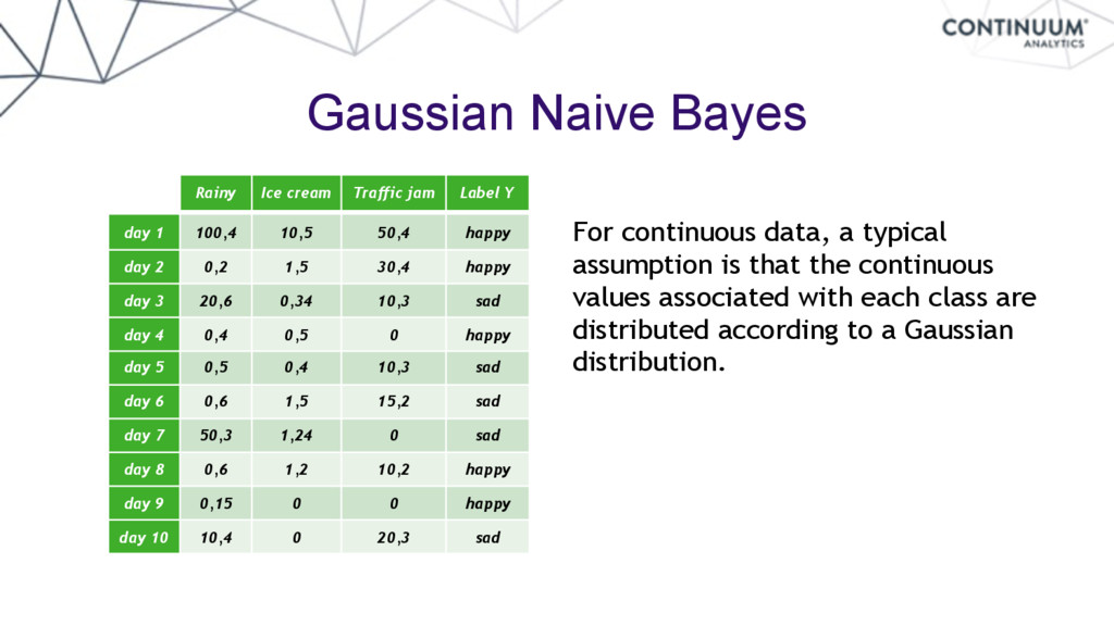
39. Gaussian Naive Bayes Rainy Ice cream Traffic jam Label Y day 1 100,4 10,5 50,4 happy day 2 0,2 1,5 30,4 happy day 3 20,6 0,34 10,3 sad day 4 0,4 0,5 0 happy day 5 0,5 0,4 10,3 sad day 6 0,6 1,5 15,2 sad day 7 50,3 1,24 0 sad day 8 0,6 1,2 10,2 happy day 9 0,15 0 0 happy day 10 10,4 0 20,3 sad For continuous data, a typical assumption is that the continuous values associated with each class are distributed according to a Gaussian distribution.
40. RECAP
41. Naive Bayes :) • Inference is cheap - Fast! • Few parameters • Empirically successful classifier
42. Naive Bayes :( • Assumes independence of features – Doesn’t model interrelationships between attributes • Bad estimator, so the probability outputs are not really useful
43. 43 Classification Discrete-valued inputs (X) Continuous inputs (X) MultinomialNB BernouilliNB GaussianNB Naive Bayes Algorithms occurance counts binary/boolean features
44. Thank you! :) Christine Doig Twitter: @ch_doig
45. 45 http://scikit-learn.org/stable/tutorial/text_analytics/working_with_text_data.html Scikit-learn Naive Bayes Resources http://scikit-learn.org/stable/modules/naive_bayes.html http://scikit-learn.org/stable/auto_examples/text/mlcomp_sparse_document_classification.html http://scikit-learn.org/stable/auto_examples/text/document_classification_20newsgroups.html http://scikit-learn.org/stable/auto_examples/classification/plot_classifier_comparison.html