Data Science and Decisions 2022: Week 2

Transcript

1. DATA SCIENCE AND DECISION MAKING Inference under uncertainty Will Lowe Data Science Lab, Hertie School 2022-02-16
2. PLAN 1 An important question about Freiburg Probability for uncertainty We need more than just probability Working with probabilities using Bayes inking about ‘priors’ what happens when we’re wrong
3. PARKING IN FREIBURG 2 Pay a fee or risk a ne? (Gössling et al., ) → Actions: A (pay), A (shirk) → Consequences: C (controlled), C (not) → Fee: hour of parking . (or . , . ) → Fine: parking violation E ( E in ) What to do? E[U(A)] = i U(Ci , A)P(Ci A) Parking violations
4. PARKING IN FREIBURG 3 Pay a fee or risk a ne? (Gössling et al., ) → Actions: A (pay), A (shirk) → Consequences: C (controlled), C (not) → Fee: hour of parking . (or . , . ) → Fine: parking violation E ( E in ) What to do? E[U(A)] = i U(Ci , A)P(Ci A) Well ok, but how do we do that? Utilities / losses are known but control probabilities have to be estimated A → Control probabilities are independent of my action P(C A) = P(C)
5. PARKING IN FREIBURG 3 Pay a fee or risk a ne? (Gössling et al., ) → Actions: A (pay), A (shirk) → Consequences: C (controlled), C (not) → Fee: hour of parking . (or . , . ) → Fine: parking violation E ( E in ) What to do? E[U(A)] = i U(Ci , A)P(Ci A) Well ok, but how do we do that? Utilities / losses are known but control probabilities have to be estimated A → Control probabilities are independent of my action P(C A) = P(C) → If parking violations are ubiquitous P(C ) ∝ P( ne) because in each ‘hexagon’ P( ne) = P(C , A ) = P(C A )P(A ) = P(C )P(A ) = P(C )k
6. PARKING IN FREIBURG 4 Pay a fee or risk a ne? (Gössling et al., ) → Actions: A (pay), A (shirk) → Consequences: C (controlled), C (not) → Fee: hour of parking . (or . , . ) → Fine: parking violation E ( E in ) E[U(A )] = P(C A ) + ne P(C A ) = P(C ) + ne P(C ) = ne P(C ) E[U(A )] = fee P(C A ) + fee P(C A ) = fee P(C ) + fee P(C ) = fee
7. PARKING IN FREIBURG 4 Pay a fee or risk a ne? (Gössling et al., ) → Actions: A (pay), A (shirk) → Consequences: C (controlled), C (not) → Fee: hour of parking . (or . , . ) → Fine: parking violation E ( E in ) E[U(A )] = P(C A ) + ne P(C A ) = P(C ) + ne P(C ) = ne P(C ) E[U(A )] = fee P(C A ) + fee P(C A ) = fee P(C ) + fee P(C ) = fee So for (risk neutral) parkers: → Don’t pay the fee when fee > ne P(C ) For town planners: → To dissuade parking, raise P(C ) or set ne > fee P(C ) Paper de nes ‘detection risk thresholds’
8. BEING TAKEN FOR A RIDE 5 Consistency is a virtue (Diaconis & Skyrms, ) One should also try to avoid this kind of Dutch book →
9. OK, PROBABILITY. BUT OF WHAT KIND? 6 It’s not generally true that P(C A ) = P(C ) In fact, even P(C A) is not generally enough. We want the causal e ect of A → e distribution of C that doing A generates is is causal decision theory
10. OK, PROBABILITY. BUT OF WHAT KIND? 6 It’s not generally true that P(C A ) = P(C ) In fact, even P(C A) is not generally enough. We want the causal e ect of A → e distribution of C that doing A generates is is causal decision theory P Probability decompositions don’t generally distinguish causal direction P(test, case) = P(test case)P(case) = P(case test)P(test)
11. OK, PROBABILITY. BUT OF WHAT KIND? 6 It’s not generally true that P(C A ) = P(C ) In fact, even P(C A) is not generally enough. We want the causal e ect of A → e distribution of C that doing A generates is is causal decision theory P Probability decompositions don’t generally distinguish causal direction P(test, case) = P(test case)P(case) = P(case test)P(test) C C T D єT єD єC A directed acyclic graph Causal mechanisms (the arrows) between variables (nodes) induce a probability distribution (via єC ,єD,єT) P(C, D, T) = P(T C, D)P(C D)P(D) (Pearl et al., )
12. OK, PROBABILITY. BUT OF WHAT KIND? 7 I C T D єT єD єC A directed acyclic graph a er intervention (breaking D → W) by stepping in to randomize W (єW) From this we can learn P(C do(A = ))
13. OK, PROBABILITY. BUT OF WHAT KIND? 7 I C T D єT єD єC A directed acyclic graph a er intervention (breaking D → W) by stepping in to randomize W (єW) From this we can learn P(C do(A = )) For learning these kinds of probabilities → Experiments → Other interventions, e.g. ‘natural experiments’ Observational causal analysis tries to use information from an unintervened system to learn about what this would look like. → If that’s possible, the e ect of do(W) is identi ed
14. NEWCOMB’S PARADOX 8 A ere are two boxes (A and B) and an evil genius who predicts your choices Box A: transparent with → Box B: opaque lled by the evil genius → If they predicted you will take both boxes: B is empty → If they predicted you would only take box B, B contains more One box, or two?
15. NEWCOMB’S PARKING POLICY 9 is is a fanciful rendition of a standard policy setup... A O C F C does not depend on A A O C F C depends on A
16. NEWCOMB’S PARKING POLICY 9 is is a fanciful rendition of a standard policy setup... A O C F C does not depend on A A O C F C depends on A C If the city sets things just right then A → O is perfectly o set by A → C → O It can look like A is independent of O!
17. PROBABILITY: THE OPTIONS 10 What is the relationship between → randomness (a feature of ‘the world’?) → uncertainty (a feature of an agent) → probabilities (a mathematical framework)
18. PROBABILITY: THE OPTIONS 10 What is the relationship between → randomness (a feature of ‘the world’?) → uncertainty (a feature of an agent) → probabilities (a mathematical framework) ree broad normative possibilities → Represent all uncertainty with probability (Bayesian statistics) → Represent uncertainty due to random processes with probabilities (Classical statistics, ‘frequentism’) → Probability not used to represent uncertainty (qualitative research?)
19. PROBABILITY: THE OPTIONS 10 What is the relationship between → randomness (a feature of ‘the world’?) → uncertainty (a feature of an agent) → probabilities (a mathematical framework) ree broad normative possibilities → Represent all uncertainty with probability (Bayesian statistics) → Represent uncertainty due to random processes with probabilities (Classical statistics, ‘frequentism’) → Probability not used to represent uncertainty (qualitative research?) Dutch book type arguments say: use probability to → represent all kinds of uncertainty (be a Bayesian) → model the decision maker is is the implicit approach of most data science, and the explicit approach of most decision theory
20. ASSIGNING PROBABILITIES 11 For the Dutch book problem, they were simply elicited → a priori, or prior to seeing any data For the parking problem, probabilities were estimated → a posteriori, or in the light of data To combine the data and prior beliefs optimally we need... Bayes theorem You’re never too young to start
21. A SIMPLE LOCATION UPDATING PROBLEM 12 Assume known σx , independent observations, and normality P(x µ) = Normal(µ, σ x ) P(x , . . . x µ) = i P(xi µ) Represent uncertainty over µ in a prior P(µ) = Normal(µ , τ )
22. A SIMPLE LOCATION UPDATING PROBLEM 12 Assume known σx , independent observations, and normality P(x µ) = Normal(µ, σ x ) P(x , . . . x µ) = i P(xi µ) Represent uncertainty over µ in a prior P(µ) = Normal(µ , τ ) See x , e.g. . and update our uncertainty to a posterior P(µ x ) = P(x µ)P(µ) ∫ P(x µ)P(µ)dµ
23. WITH TWO DATA POINTS 13 What is the true mean µ of x? Assume known σx , independent observations, and normality P(x µ) = Normal(µ, σ x ) P(x , . . . x µ) = i P(xi µ) Since these observations are independent we can process them all at once P(µ, x , x ) = P(x µ)P(x µ)P(µ) ∫ P(x µ)P(x µ)P(µ)dµ = ∏i P(xi µ)P(µ) ∫ ∏i P(xi µ)P(µ)dµ
24. WITH TWO DATA POINTS 14 What is the true mean µ of x? Assume known σx , independent observations, and normality P(x µ) = Normal(µ, σ x ) P(x , . . . x µ) = i P(xi µ) or sequentially, using the old posterior as a prior P(µ, x , x ) = P(x µ, x )P(µ x ) ∫ P(x µ, x )P(µ x )dµ = P(x µ)P(µ x ) ∫ P(x µ)P(µ x )dµ
25. AS COMPROMISE 15 Call the posterior mean and variance a er seeing k data points µk and τk A precision-weighted average µ = τ µ + σx x τ + σx and with all ten observations µ = τ µ + σx ¯ x τ + σx Note: Here only the x average matters as shrinkage of data towards µ µ = x − σx σx + τ (x − µ )
26. AS COMPROMISE 16 Call the posterior mean and variance a er seeing k data points µk and τk A precision-weighted average µ = τ µ + σx x τ + σx and with all ten observations µ = τ µ + σx ¯ x τ + σx Note: precision = /variance Adjust beliefs about µ from data µ = µ + τ σx + τx (x − µ )
27. STATE SPACE SYSTEMS 17 M Keep everything the same as before but let P(µ(t+ ) µ(t)) = Normal(µ(t), σµ) en the adjustment to our posterior over µ is slightly more complicated, but the mean still has the form µt = µt− + K (xt− − µt− ) where K is a ‘gain’ that weights the ‘observation error’ or ‘innovation’ at t is Kalman Filter is Bayesian updating forthe linear normal state space model Good enough to land Apollo on the moon in
28. STATE SPACE SYSTEMS 18 Still basis of most missiles (and missile tracking systems), driverless car so ware, robotics, etc.
29. INTUITIONS 19 C As we get more and more observations what happens to the in uence of the prior?
30. INTUITIONS 19 C As we get more and more observations what happens to the in uence of the prior? In this example P(µ x . . . xn) ≈ Normal(¯ x, σx n) (for τ xed as n → ∞ and for n xed as τ → ∞) → Remind you of anything you’ve seen before?
31. INTUITIONS 19 C As we get more and more observations what happens to the in uence of the prior? In this example P(µ x . . . xn) ≈ Normal(¯ x, σx n) (for τ xed as n → ∞ and for n xed as τ → ∞) → Remind you of anything you’ve seen before? For large enough n the sampling distribution of the average is ¯ x ∼ Normal(µ, σx n) so we’d agree that ¯ x is a useful estimate (as well as being the posterior mean) Note: is kind of happy agreement is not as common as we might like
32. INTUITIONS 20 M What happens if µ is just really far away from µ?
33. INTUITIONS 20 M What happens if µ is just really far away from µ? What quantities determine how fast it gets closer to right? → How could we make it get there faster? If σx = τ how much information is there in the prior? → How could we make a less informative prior? → Could we imagine a completely uninformative prior?
34. UNINFORMATIVENESS 21 I → Informativeness is proportional to atness A subtle problem with the original idea → Flatness can be relative to parameterization E → What proportion of respondents are vaccinated? → What is the probability a person is infected? Possible prior parameterizations to be at in: → Probability: π → Logit: ϕ = log π −π (Lunn et al., )
35. CHOOSING PRIORS 22 Bayesian probability is personal (that’s why we’re looking at in a decision course) ‘Personal’ can be ambiguous → a model of certainty that is idiosyncratic, quirky, etc. (not really) → a model of uncertainty that actual people have? (the jury is still out) → a model of uncertainty that people should have? maybe! → a model of uncertainty that people could have Let’s look at the last one in more detail (Lunn et al., )
36. RULING THINGS OUT 23 What happens to the posterior if the prior says P(µ > . ) = (It certainly can’t be Normal, but what else?)
37. RULING THINGS OUT 24 Knowing that probability will converge at the ‘edge’ of the prior support closest to truth... may not be very reassuring We can be redeemably and irredeemably wrong → Prior is bad but (eventually) data will brings us to the truth → Prior is bad and we cannot get there from here More on the applications consequences of this later...
38. DIAGNOSING WRONGNESS 25 Previously we asked: what happens to the posterior if the prior says P(µ > . ) = e general problem here is Bayes’ natural assumption of a closed world → You can only update on things that you believe are possible Baggy Robot Ninja Pedestrians
39. CLOSED WORLD ASSUMPTIONS 26 e view from the other side (Frequentism) → Only put probability on things that were sampled / randomized / could have gone di erently / non-mental → Generate estimators (procedures with guarantees, not distributions with properties) → Test hypotheses, o en (Fisher) with unstated alternatives Oh hai
40. TRACKING THE WORLD 27 We can also demand coverage for intervals and calibration for predictions Calibration (for classi ers): → If a classi er says: P(recidivism) = . then ≈ % of people predicted to recidivize(?) do so Bayes does not, in general, guarantee this
41. SUMMING UP 28 Bayes is crazy powerful framework for uncertainty quanti cation Expressing serious uncertain is harder that you might imagine Expressing impossibility might be a bit too easy Realistic decision models imply computation (potentially a lot) e ‘lump of probability’ (total volume ) is only so big and if you forget to spread it around far enough, you may not nd out
42. (NEARLY) ALL OF ML 29 You can do basically all of Machine Learning with this machinery If you’d like a taste, a dra Intro version of this book is available here: https://probml.github.io/pml-book/
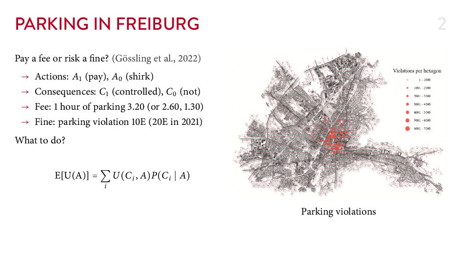
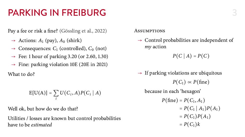
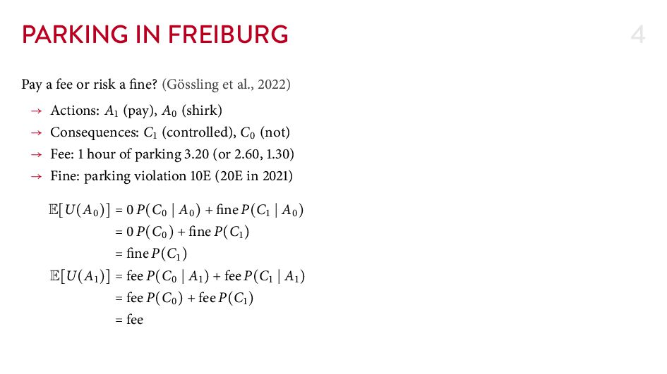
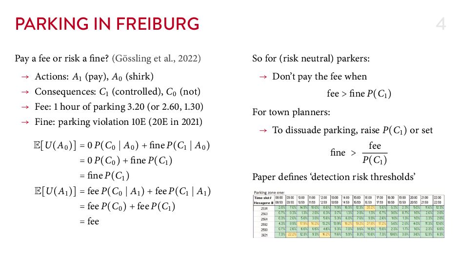
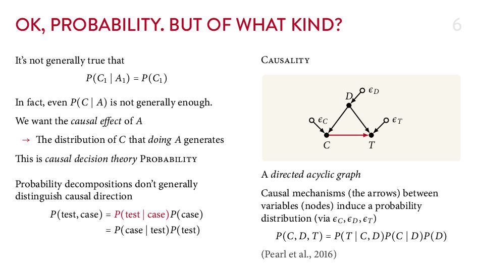
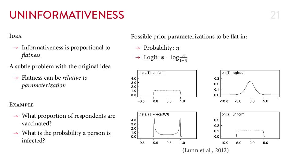
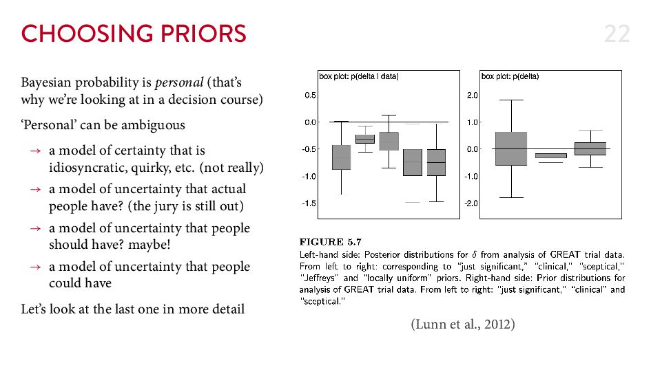
43. REFERENCES 30 Diaconis, P., & Skyrms, B. ( ). “Ten great ideas about chance.” Princeton University Press OCLC: ocn . Gössling, S., Humpe, A., Hologa, R., Riach, N., & Freytag, T. ( ). “Parking violations as an economic gamble for public space.” Transport Policy, , – . Lunn, D., Jackson, C., Best, N., omas, A., & Spiegelhalter, D. ( ). “ e BUGS book: A practical introduction to Bayesian analysis.” CRC Press. Pearl, J., Glymour, M., & Jewell, N. P. ( ). “Causal inference in statistics: A primer.” Wiley.