An introduction to the IOx Read Buffer (an in-memory execution engine)

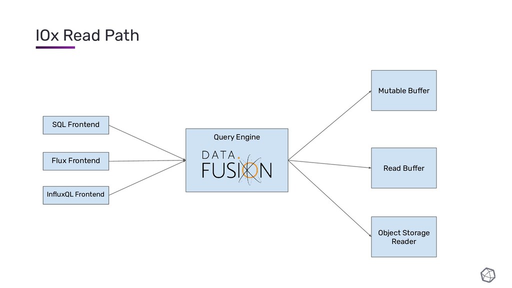
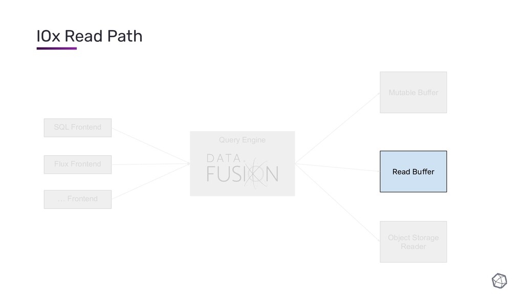
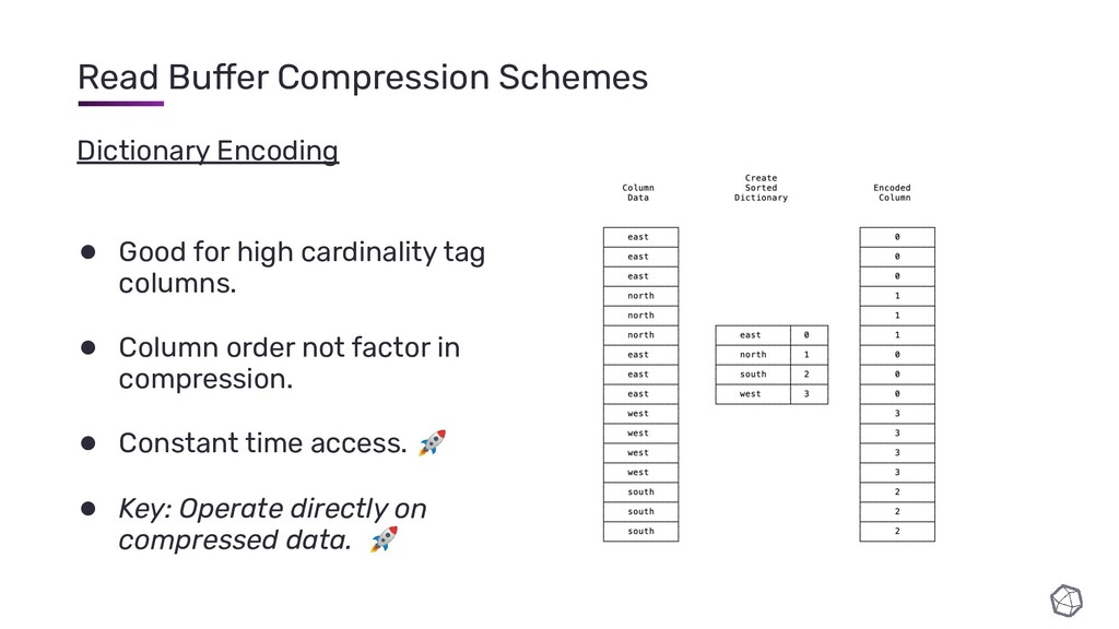
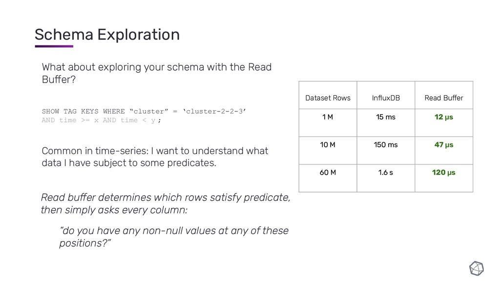
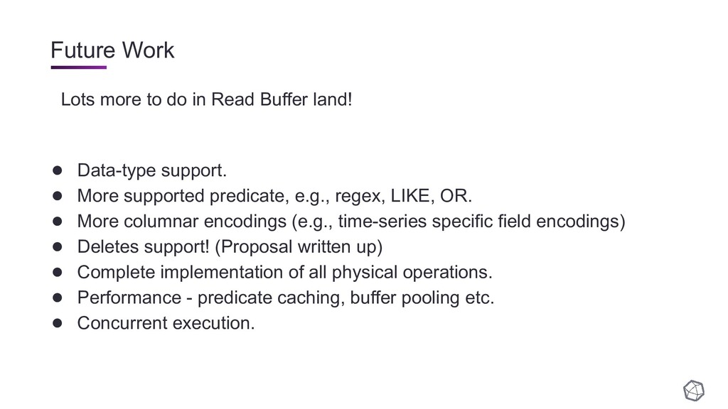
These slides are from a talk I gave about InfluxDB IOx's Read Buffer, a query execution engine that I have been building in Rust.

Talk here: https://youtu.be/KslD31VNqPU

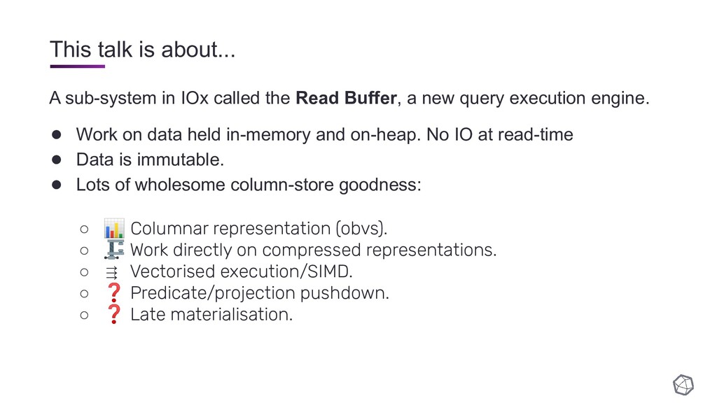
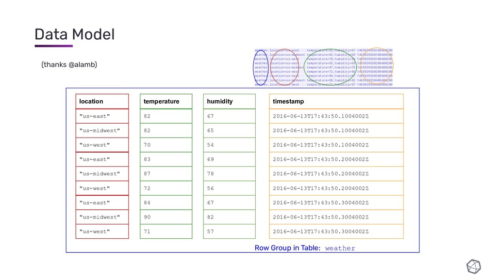
You might find this interesting if you're interested in column-oriented databases, time-series databases or general analytical data processing.

Transcript

1. Edd Robinson Engineer @ InfluxData edd@influxdata.com @e-dard 🐙 @eddrobinson 🐦 An Intro to the InfluxDB IOx Read Buffer: a read-optimised in-memory execution engine
2. Me • Software engineer at InfluxData. • Worked on InfluxDB for ~4y: storage engine, write path, indexing. Working on IOx (and with Rust!) for just over a year.
3. What are we working towards? Some performance/scalability goals: • Unlimited Data: ◦ Object Storage, compression • Unlimited Cardinality: ◦ Data organisation, no large indexes. • 🚀 Analytical Queries: ◦ in-memory, columnar data-layout, lots of fanciness
4. This talk is about... A sub-system in IOx called the Read Buffer, a new query execution engine. • Work on data held in-memory and on-heap. No IO at read-time • Data is immutable. • Lots of wholesome column-store goodness: ◦ 📊 Columnar representation (obvs). ◦ 🗜 Work directly on compressed representations. ◦ ⇶ Vectorised execution/SIMD. ◦ ❓ Predicate/projection pushdown. ◦ ❓ Late materialisation.
5. Wider Goals We want to have excellent support for different time-series use-cases • Events • Observability trifecta (logging, tracing, metrics) • Large analytical workloads
6. We already have a time-series database?
7. Quick Refresher • IoT, monitoring or other time-series use-cases. • Excellent block-compression of most field and timestamp data. • Flexible data model. • Fantastic performance on selective queries. InfluxDB can handle many billions of samples over millions of series.
8. InfluxDB Happy Place ~1.8GB file (75MB index) 525M points 3.66 bytes per point!! Many points (samples) per series Back of envelope uncompressed block data: ~67GB Statistical TSM file analysis from IoT use-case
9. InfluxDB Sad 🐼 ~1.3 GB file (~1.1 GB index) One sample (point) per series TSM data is ~155 MB Uncompressed is ~77 MB .👎 Statistical TSM file analysis from tracing use-case - (every sample unique) N.B, there are ways around this...
10. So... • In pathological cases, index dominates and compression useless. • mmap unpredictable and can be problematic in containerised environments. • Data distribution often orthogonal to access patterns. • InfluxDB over-indexes for very high cardinality workloads and non-selective queries.
11. • Columnar architecture. Organise data in ways that make processing fast and footprint small. • Ditch the large secondary indexes. • Just say no to mmap - predictable memory usage. • Does it bring you joy? Declutter and keep only relevant data in-memory. We will excel for high-cardinality analytical workloads, and mechanical sympathy will keep us in the race on highly-selective workloads. IOx Bets
12. Why columnar is the way to go • Analytical workloads usually only need projections of dataset. • Increase flexibility in data organisation. • Improve data relevance. • Reduce footprint through compression. • Mechanical sympathy - CPUs love arrays. Forrest Smith - blog
13. Why columnar is the way to go Memory Bandwidth: benchmark • This example is synthetic (but indicative!) • Data throughput from memory to CPU has an impact on performance. • CPU cache is significantly faster than main memory
14. Why columnar is the way to go L1 Cache L2/L3 Cache Main Memory Memory Bandwidth: benchmark • This example is synthetic (but indicative)! • Data throughput from memory to CPU has an impact on performance. • CPU cache is significantly faster than main memory If you want to make the most use of your memory bandwidth: • process less data. • process more relevant data. Columnar representations help with both of these
15. 🤿 Dive into the Read Buffer Rest of the talk focuses on: • Data organisation; • Data representation; • Read execution (late materialisation); • Early numbers! • Future improvements.
16. • WAL: replication and recovery • Mutable Buffer: query written data • Object Store: for durability • Read Buffer: optised read-only view of written data. IOx Write Path
17. IOx Read Path Query Engine SQL Frontend Flux Frontend InfluxQL Frontend Mutable Buffer Read Buffer Object Storage Reader
18. IOx Read Path Query Engine SQL Frontend Flux Frontend … Frontend Mutable Buffer Read Buffer Object Storage Reader
19. Data Model Data organised by database
20. Data Model Databases are collections of partitions Partition Key
21. Chunk ID Data Model Partitions contain chunks
22. Table name Data Model Chunks contain Tables
23. Data Model Tables contain Row Groups Same Schema Filter entire tables
24. Data Model Row Groups contain columnar data Skip Row Group
25. Data Model (thanks @alamb) weather,location=us-east temperature=82,humidity=67 1465839830100400200 weather,location=us-midwest temperature=82,humidity=65 1465839830100400200 weather,location=us-west temperature=70,humidity=54 1465839830100400200 weather,location=us-east temperature=83,humidity=69 1465839830200400200 weather,location=us-midwest temperature=87,humidity=78 1465839830200400200 weather,location=us-west temperature=72,humidity=56 1465839830200400200 weather,location=us-east temperature=84,humidity=67 1465839830300400200 weather,location=us-midwest temperature=90,humidity=82 1465839830400400200 weather,location=us-west temperature=71,humidity=57 1465839830400400200 location "us-east" "us-midwest" "us-west" "us-east" "us-midwest" "us-west" "us-east" "us-midwest" "us-west" temperature 82 82 70 83 87 72 84 90 71 humidity 67 65 54 69 78 56 67 82 57 timestamp 2016-06-13T17:43:50.1004002Z 2016-06-13T17:43:50.1004002Z 2016-06-13T17:43:50.1004002Z 2016-06-13T17:43:50.2004002Z 2016-06-13T17:43:50.2004002Z 2016-06-13T17:43:50.2004002Z 2016-06-13T17:43:50.3004002Z 2016-06-13T17:43:50.3004002Z 2016-06-13T17:43:50.3004002Z Row Group in Table: weather
26. Supported Data Types Logical Data Types • String (utf-8 valid strings) • Float (double-precision float) (all of them 😉) • Integer (signed integers) • Unsigned (unsigned integers) • Boolean • Binary (arbitrary bytes) Semantic Column Types • InfluxDB Tag ➟ String • InfluxDB Field ➟ Most • InfluxDB Timestamp ➟ I64 • IOx Column ➟ Anything
27. Tailored for time-series: • scans, grouped aggregates, windowed aggregates, schema exploration (tables, columns, values). • Table/row group pruning. • Predicate pushdown. • Comparator operators with constant on tag columns (<, <=, >, >=, =, !=} • Aggregates any column(s) Interesting Supported Features
28. Storing Data in the Read Buffer ➡
29. Columnar Compression Spectrum Lots ‘o Compression 💯 Smaller Footprint 👎 High processing cost No Compression 👎 Larger footprint 💯 ~Zero processing cost
30. Columnar Compression Spectrum Lots ‘o Compression Smaller Footprint High processing cost No Compression Larger footprint ~Zero processing cost Vec<T> zstd lz4 gzip snappy Dictionary Encoding Run-length Encoding Trim bits “TS compression” e.g., gorilla, simple8b
31. Choice can depend on data location xxx MB/s x GB/s xx GB/s
32. And Medium $$$ Petabytes $0.03/GB Gigabytes $10/GB?? Terabytes $0.1/GB xxx MB/s x GB/s xx GB/s
33. Read Buffer Compression Schemes Dictionary Encoding • Good for high cardinality tag columns. • Column order not factor in compression. • Constant time access. 🚀 • Key: Operate directly on compressed data. 🚀
34. Read Buffer Compression Schemes Filtering Dictionary Encoding WHERE “region” = ‘east’ Predicate Consult Dictionary Encoded Column Apply Encoded Predicate x = 0 {0, 2, 7, 15} WHERE “region” > ‘north’ x > 1 {1, 3, 5, 8, 9, 10, 11, 12, 14}
35. “RLE” - Run-Length Encoding • Incredible compression when lots of “runs”. • Works best on heavily sorted columns. • Not as consumable* • Pre-computed bitsets 🚀 • Can operate on compressed data. 🚀 Read Buffer Compression Schemes
36. Read Buffer Compression Schemes “RLE” - Run-Length Encoding WHERE “region” = ‘east’ Predicate Consult Dictionary Encoded Column Lookup pre-computed bitset x = 0 WHERE “region” > ‘north’ Iterate run-lengths or union bitmaps x > 1 {9, 10, 11, 12, 13, 14, 15}
37. Which Dictionary Encoding? Filtering WHERE “region” = ‘east’ • 10M rows in column • Cardinality 10,000 • Single thread Billions rows/second processed
38. Which Dictionary Encoding? Filtering WHERE “region” = ‘east’ • 10M rows in column. • Cardinality 10,000. • Single thread. • SIMD intrinsics on Dictionary Encoding. • RLE is on another level: “cheating”... Billions rows/second processed RLE 59ms 2.2ms 420ns 380MB ~40MB ~40MB
39. Which Dictionary Encoding? Filtering - high cardinality WHERE “span_id” = ‘123djk7GHs99wj’ • 10 million rows in column. • Cardinality 10 million. • Single thread. • SIMD intrinsics on Dictionary Encoding. Billions rows/second processed RLE 60ms 2.2ms 380MB ~420MB RLE still on another level, but look at the memory... 580ns ~1GB
40. Which Dictionary Encoding? What about materialisation? “I need rows [2, 33, 55, 111, 3343]” 10,000,000 row column Encoding Cardinality 10K (materialise 1000 rows near end) Cardinality 10M (materialise 1 row near end) Vec<String> 747 ns 66 ns Dictionary 2.4 μs 189 ns RLE 7.4 μs 6.4 ms
41. Which Dictionary Encoding? Summary • Working on compressed data provides benefit over raw representation: small fixed size, SIMD, integer math etc. • RLE can be incredibly performant for filtering, but size can grow… • Dictionary filtering performance proportional to column size, but materialisation always performant.
42. Numerical Column Encodings Supported Logical types: i64, u64, f64 Internally, Read Buffer automatically converts to: {u8, i8,.., u64, i64}* Example: &[i64]: (48 B) [123, 198, 1, 33, 133, 224] ➠ &[u8]: (6 B) [..] &[i64]: (48 B) [-18, 2, 0, 220, 2, 26] ➠ &[i16]: (12 B) [..]
43. Numerical Column Encodings Timestamps, counters and XYZ are really big though! N.B., Soon • There are lightweight ways to compress data leveraging its shape. • E.g., frame-of reference, divide by common denominator. • Important to keep constant-time access. • Aiming to avoid “block-based” time-series compression.
44. Read Execution Consider the scan operation for: SELECT “host”, “counter”, “time” FROM “cpu” WHERE “env” = ‘prod’ AND “path” = ‘/write’ AND “counter” > 200 AND “time” >= x AND “time” < y; High level steps: • Can we prune entire chunks? • Can we prune entire row groups from tables? • Gather row groups for processing, build result schema. • Process row groups....
45. Late Materialisation - Scanning Filtering on compressed data compressed sets of ordinal offsets (row ids) Integer set operations - fast! Materialise values at row positions SELECT “host”, “counter”, “time” FROM “cpu” WHERE “env” = ‘prod’ AND “path” = ‘/write’ AND “counter” > 200 AND “time” >= x AND “time” < y;
46. Late Materialisation - Grouping SELECT SUM(“counter”) FROM “cpu” WHERE “path” = ‘/query’ AND “time” >= x AND “time” < y GROUP BY “region”; Integer keys = ♥ Filtering on compressed data Use offsets to get compressed values Materialise group key values
47. Let’s look at some initial numbers
48. • Simulate tracing data across distributed system. • Effectively “unlimited” cardinality as every row contains unique span_id. • Data sorted low-high; traces/spans scattered... • Query patterns mixed. • Most columns would be stored in InfluxDB as tags (possible to do fields too). Synthetic High Cardinality Tracing use-case Column Name Cardinality Encoding env 2 RLE data_centre 20 RLE cluster 200 RLE node_id 2,000 RLE pod_id 20,000 RLE user_id 200,000 Dictionary request_id 2,000,000 Dictionary trace_id 10,000,000 Dictionary span_id Unique (∞) Dictionary duration (u64) N/A Numeric (u32) timestamp (i64) N/A Numeric (i64)
49. How much space do we need? • Loaded datasets into InfluxDB and Read Buffer. • 1M rows, 10M rows, ~60M rows* • Fully compacted InfluxDB/re-built indexes “best case”.
50. How much space do we need? • Loaded datasets into InfluxDB and Read Buffer. • 1M rows, 10M rows, ~60M rows* • Fully compacted InfluxDB/re-built indexes “best case”. The Read Buffer upto ~10x smaller footprint than InfluxDB.
51. Dataset Rows InfluxDB Read Buffer 1 M 1 ms 1.2 ms 10 M 1.1 ms 2.5 ms 60 M 1.3 ms 15.7 ms Let’s look at a very selective operation… SELECT * FROM “traces” WHERE “trace_id” = ‘H7whivfl’; • 0.00002–0.001% rows match • An index would be good 🤔 • How far will brute force get us? 💪 • Just being in the ballpark is “Needle in a Haystack” Read buffer performance scales well with dataset size...
52. Now something that needs to process all rows and aggregate a certain column. SELECT SUM(duration) FROM “traces” GROUP BY “trace_id”; • As in: “what are my slowest/fastest traces?” • Produces up to 10M groups. • Heads up - InfluxDB is not suited to this... Aggregating over high-cardinality Dataset Rows InfluxDB Read Buffer 1 M 30 s (~10 GB RAM) 45 ms (8 MB) 10 M 18 min (140 GB RAM) 498 ms (150 MB) 60 M D.N.F (OOM) 4.3 s (900MB) Read buffer can execute these operations well beyond where InfluxDB stops
53. What about exploring your schema with the Read Buffer? SHOW TAG KEYS WHERE “cluster” = ‘cluster-2-2-3’ AND time >= x AND time < y ; Common in time-series: I want to understand what data I have subject to some predicates. Schema Exploration Dataset Rows InfluxDB Read Buffer 1 M 15 ms 12 μs 10 M 150 ms 47 μs 60 M 1.6 s 120 μs Read buffer determines which rows satisfy predicate, then simply asks every column: “do you have any non-null values at any of these positions?”
54. Future Work Lots more to do in Read Buffer land! • Data-type support. • More supported predicate, e.g., regex, LIKE, OR. • More columnar encodings (e.g., time-series specific field encodings) • Deletes support! (Proposal written up) • Complete implementation of all physical operations. • Performance - predicate caching, buffer pooling etc. • Concurrent execution.
55. Thank You