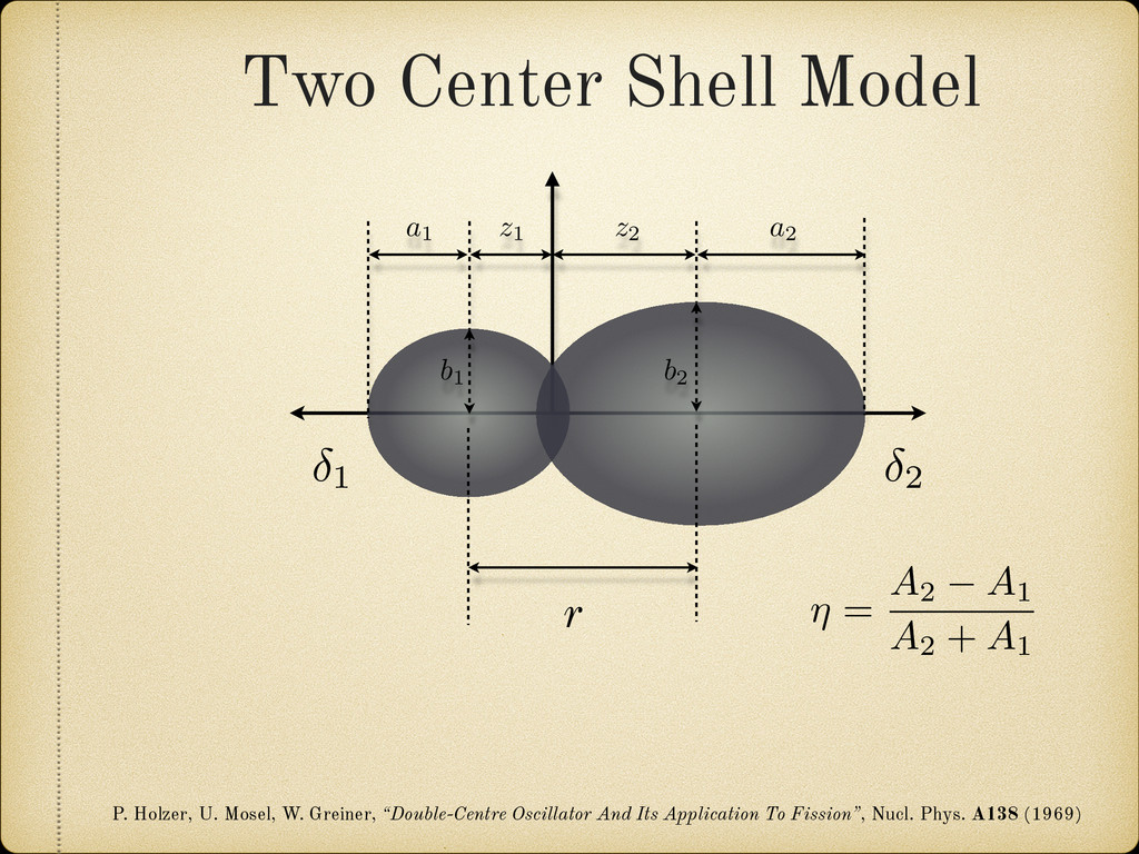
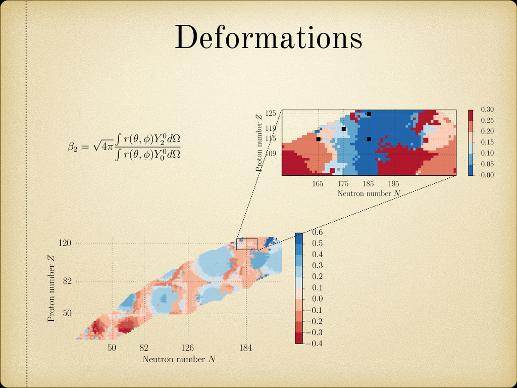
the elongation, asymmetry, neck, and fragment deformations as natural parameters to characterize the nuclear shape, we have calculated the quadrupole deformation 2 of the spherical harmonic expansion for easier comparison with previous theoretical calculations. This de- formation parameter is defined by: 2 = p 4⇡ R r(✓, )Y 0 2 d⌦ R r(✓, )Y 0 0 d⌦ where r(✓, ) is the radius vector describing the nuclear surface. In Figure 2.19 the obtained 2 values are plotted against Z and N. It can be observed how in general the sphericity of the proton shells fades a lot faster than the neutron ones when we move away from the corresponding magic number. In fact in some cases it vanishes completely, like in the region between the neutron shells Z = 126 and Z = 184. formation Two Center Shell Model uses the elongation, asymmetry, neck, and ormations as natural parameters to characterize the nuclear shape, ulated the quadrupole deformation 2 of the spherical harmonic easier comparison with previous theoretical calculations. This de- rameter is defined by: 2 = p 4⇡ R r(✓, )Y 0 2 d⌦ R r(✓, )Y 0 0 d⌦ is the radius vector describing the nuclear surface. 2.19 the obtained 2 values are plotted against Z and N. It can be in general the sphericity of the proton shells fades a lot faster than nes when we move away from the corresponding magic number. In cases it vanishes completely, like in the region between the neutron 6 and Z = 184.
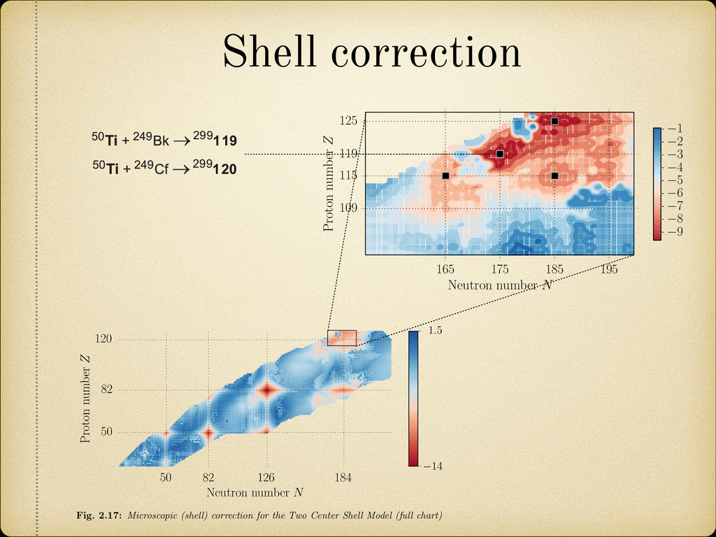
Center Shell Model (full chart) Fig. 2.17: Microscopic (shell) correction for the Two Center Shell Model (full chart) 165 175 185 195 Neutron number N 109 115 119 125 Proton number Z 9 8 7 6 5 4 3 2 1 Fig. 2.18: Microscopic (shell) correction for the Two Center Shell Model (superheavy region) 41 re 4. Predicted cross sections for synthesis of element 119 and 120 in the 50Ti + 249Bk (a), + 249Cf (b) and 54Cr + 248Cm (c) fusion reactions. The arrows indicate the upper limits ed in the experiments performed at GSI by beginning of June 2012. sotopes of SH elements with Z>120 produced in these reactions could be shorter than a microseconds, time needed for SH nucleus to pass through separator. Thus, the production elements with Z>120 looks rather vague in the nearest future. The use of radioactive ion s does not solve this problem [13]. ons for synthesis of element 119 and 120 in the 50Ti + 249Bk (a), Cm (c) fusion reactions. The arrows indicate the upper limits ormed at GSI by beginning of June 2012. h Z>120 produced in these reactions could be shorter than a or SH nucleus to pass through separator. Thus, the production s rather vague in the nearest future. The use of radioactive ion
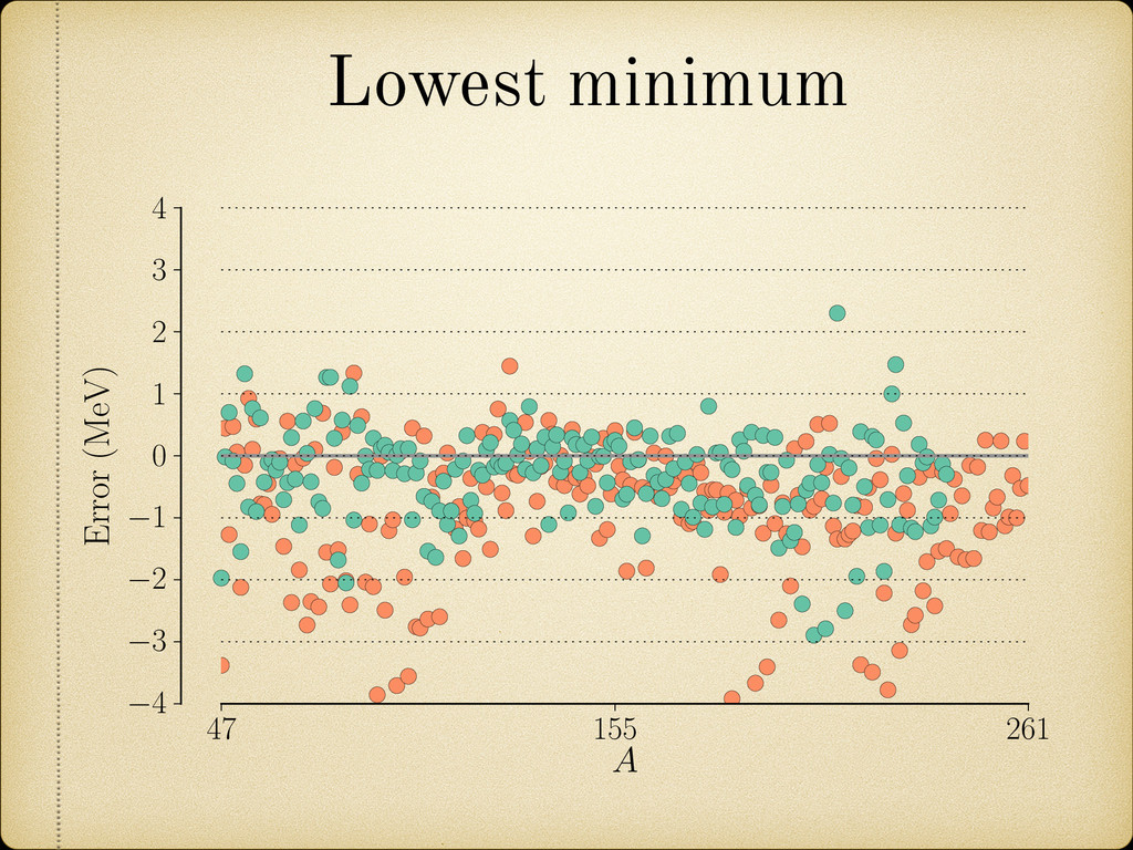
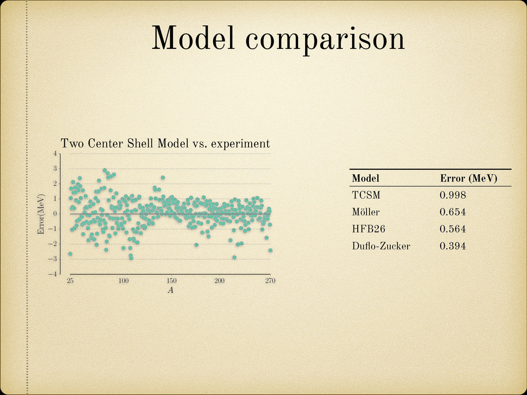
(for example a growing pattern) as this would mean that we can not rely on the future behavior of the model when it is used to extrapolate in the unknown region. 25 100 150 200 270 A 4 3 2 1 0 1 2 3 4 Error(MeV) Fig. 2.12: Sample of the mass difference (error) scatter of the theoretically calculated mass excess compared to experimental results from Audi 2012 [2]. In Figure 2.13 we present a nuclear chart showing the distribution of the error for different regions. It can be observed that the TCSM predicts higher values of the binding energies (lower mass excess) in the regions around both proton and neutron closed shells. This is more closely illustrated in Figure 2.14. This plot also shows an oscillating behavior between neighboring nuclei which points to the need of a correction in the pairing energy. On the positive side this overestimation of the binding energies remains small (< 1.5 MeV) most of the Two Center Shell Model vs. experiment Model Error (MeV) TCSM 0.998 Möller 0.654 HFB26 0.564 Duflo-Zucker 0.394
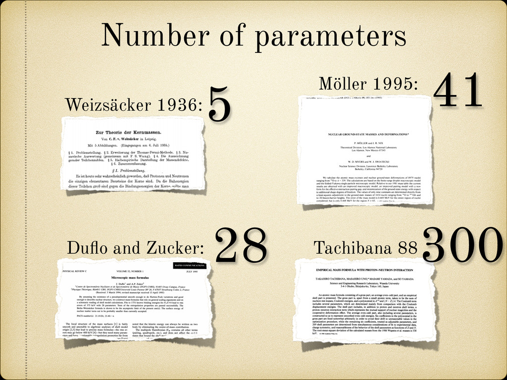
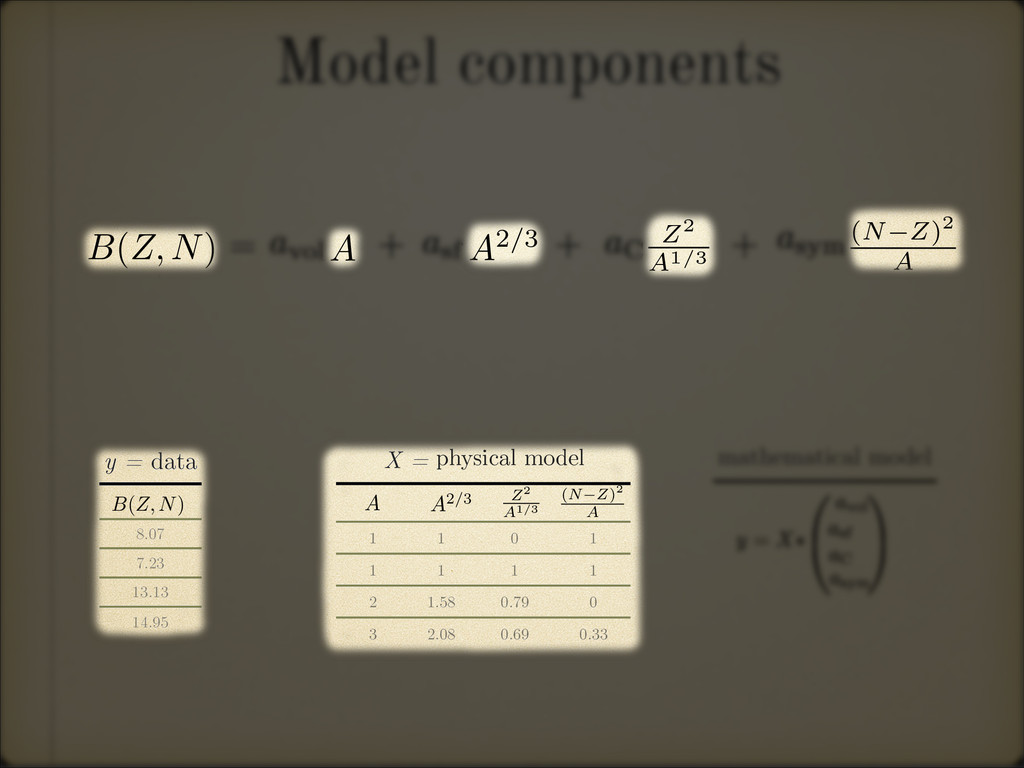
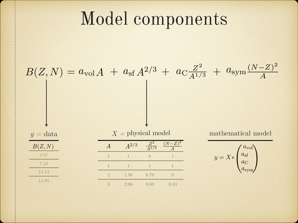
+ asym (N Z)2 A B(Z, N) = Model components X = 1 1 0 1 1 1 1 1 2 1.58 0.79 0 3 2.08 0.69 0.33 (N Z)2 A A A2/3 Z2 A1/3 y = data 8.07 7.23 13.13 14.95 B(Z, N) a vol asf aC asym y = X⇤ mathematical model physical model
+ asym (N Z)2 A B(Z, N) = Model components X = 1 1 0 1 1 1 1 1 2 1.58 0.79 0 3 2.08 0.69 0.33 (N Z)2 A A A2/3 Z2 A1/3 y = data 8.07 7.23 13.13 14.95 B(Z, N) a vol asf aC asym y = X⇤ mathematical model physical model
+ asym (N Z)2 A B(Z, N) = Model components X = 1 1 0 1 1 1 1 1 2 1.58 0.79 0 3 2.08 0.69 0.33 (N Z)2 A A A2/3 Z2 A1/3 y = data 8.07 7.23 13.13 14.95 B(Z, N) a vol asf aC asym y = X⇤ mathematical model physical model
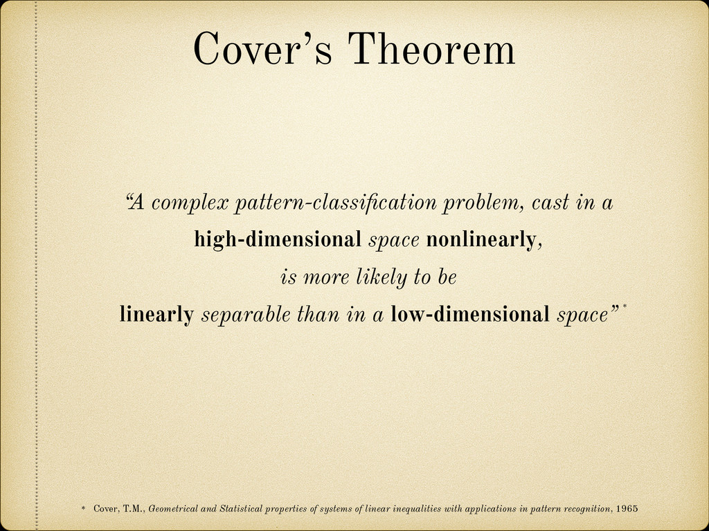
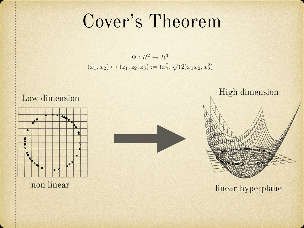
is more likely to be linearly separable than in a low-dimensional space” Cover, T.M., Geometrical and Statistical properties of systems of linear inequalities with applications in pattern recognition, 1965 Cover’s Theorem * *
compare models that had “access” to more data to older models without this privilege, it can be argued that a good model shouldn’t really depend much on the subset of the data it is being trained to. In second place if we constrain our comparisons to the predicted results and not to the underlying models themselves then the comparison becomes fair as we are only evaluating how correct the actual predicted values are. AME95 AME03 AME12 SVM13 0.241 0.239 0.251 FRDM95 0.678 0.656 0.654 HFB26 0.574 0.571 0.564 DUZU 0.346 0.360 0.394 Table 3.5: Root mean squared errors for several theoretical predictions models. See [8] for references to the models. Accuracy Root mean squared error (MeV)
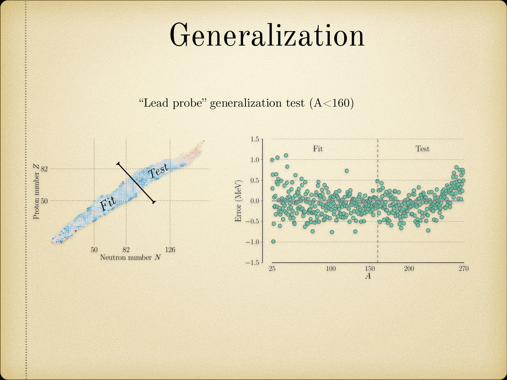
0.5 1.0 1.5 Error (MeV) Fit Test Fig. 3.26: Error profile for the “lead probe region” is in line with the observations of refrence [115] where all models perceived an increase in error by a factor of 1.4-4. We start to see a systematic deviation into positive values of the error starting around A = 240. This means that the model behaves reliably with only a small decrease in performance in an interval almost 80 units away from the region it was fitted. 3.4.5 Half-lives for ↵-decay Generalization “Lead probe” generalization test (A<160) 50 82 126 Neutron number N 50 82 Proton number Z 1.06 1.51 Fit Test
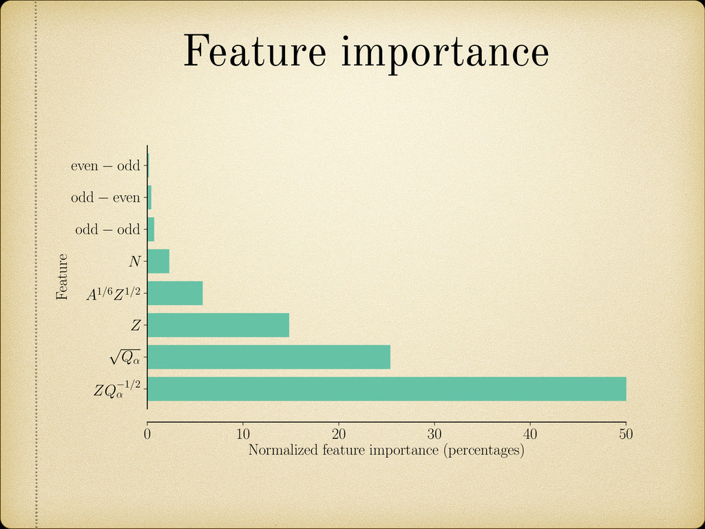
alpha decay can be described quantum tunneling effect, Geiger and Nuttal [122] observed that there was mple dependence between the mean reach of a alpha particles in air and t ean decay constant. This relationship was generalized in 1966 by Viola an eaborg to the form: log 10 [T ↵ (VSS)] = (aZ + b)Q 1/2 ↵ + cZ + d + h log (3. here T ↵ is given in seconds and Q ↵ is given in MeV. The coefficients we ted by Sobiczewski to even-even nuclei [11], obtaining the values shown ble Table 3.7. even-even even-odd odd-even odd-odd hlog 0 1.066 0.772 1.114 a b c d 1.66175 -8.5166 -0.20228 -33.9069 Table 3.7: Coefficients for the Viola and Seaborg [11] formula odd-odd -29.48 -1.113 1.6971 Table 3.8: Coefficients for the Royer [12] formula he Sobiczewski-Parkhomenko formula he 5 parameter formula4 from Sobiczewski and Parkhomenko was taken fro 3] and has the form: log 10 [T ↵ (SP)] = aZ(Q ↵ E i ) 1/2 + bZ + c (3 ith the set of parameters a = 1.5372, b = 0.1607 and c = 36.573. epresents the average excitation energy of a state of the daughter nucleus; t orresponding values are tabulated in Table 3.9. These parameters were obtain even-even even-odd odd-even odd-odd E i 0 0.171 0.113 0.284 hlog 0 1.066 0.772 1.114 a b c d 1.66175 -8.5166 -0.20228 -33.9069 Table 3.7: Coefficients for the Viola and Seaborg [11] formula Royer’s formula or the Royer formula we will use the form given in [12], log 10 [T ↵ (Royer)] = a + bA1/6 Z1/2 + cZQ 1/2 ↵ (3. ith coefficients given in Table 3.8. Sobiczewski-Parkhomenko Viola and Seaborg Royer’s formula G. Royer, “Alpha emission and spontaneous fission through quasi-molecular shapes,” Journal of Physics G (2000) A. Sobiczewski, Z. Patyk, and S. Ćwiok, “Deformed superheavy nuclei,” Physics Letters B (1989) A. Parkhomenko and A. Sobiczewski, “Phenomenological formula for alpha-decay half-lives of heaviest nuclei,” Acta physica polonica B (2005)
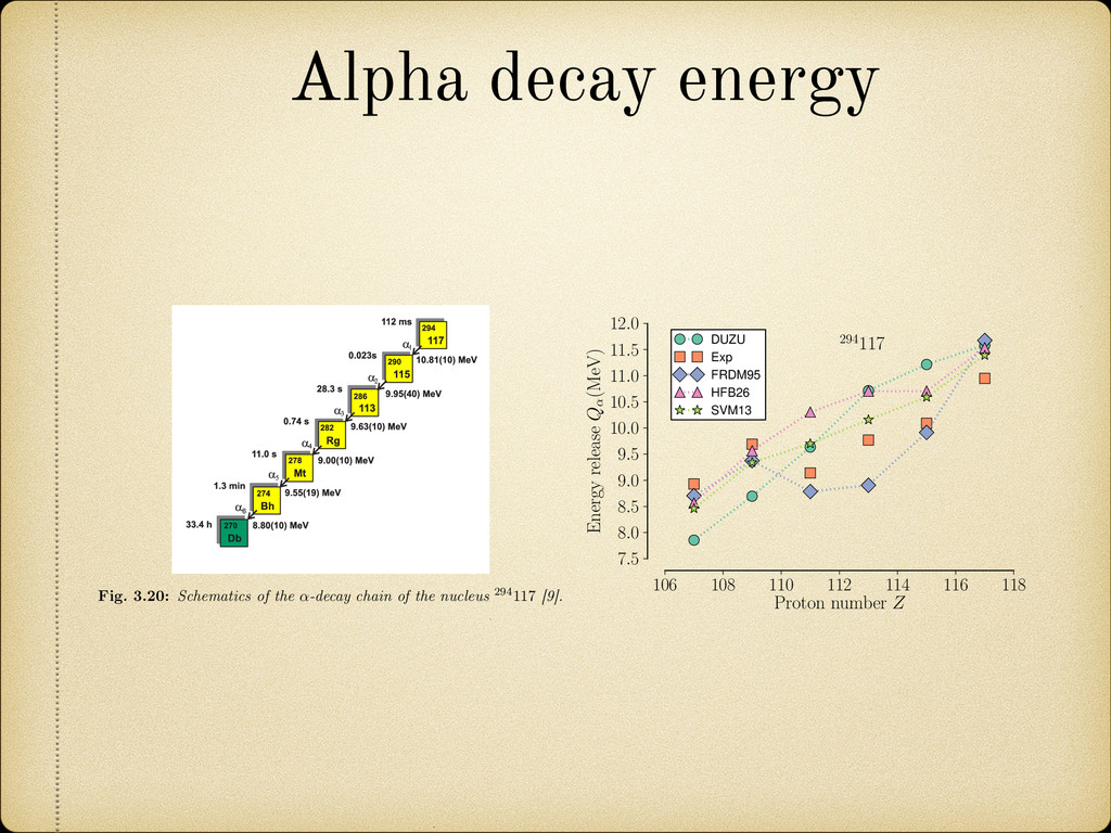
294 117 [9]. 106 108 110 112 114 116 118 Proton number Z 7.5 8.0 8.5 9.0 9.5 10.0 10.5 11.0 11.5 12.0 Energy release Q↵(MeV) 294117 DUZU Exp FRDM95 HFB26 SVM13 Fig. 3.21: Prediction of several theoretical models for the Q ↵ energies of the ↵-decay chain of the nucleus 294 117 79 Alpha decay energy Fig. 3.20: Schematics of the ↵-decay chain of the nucleus 294 117 [9].
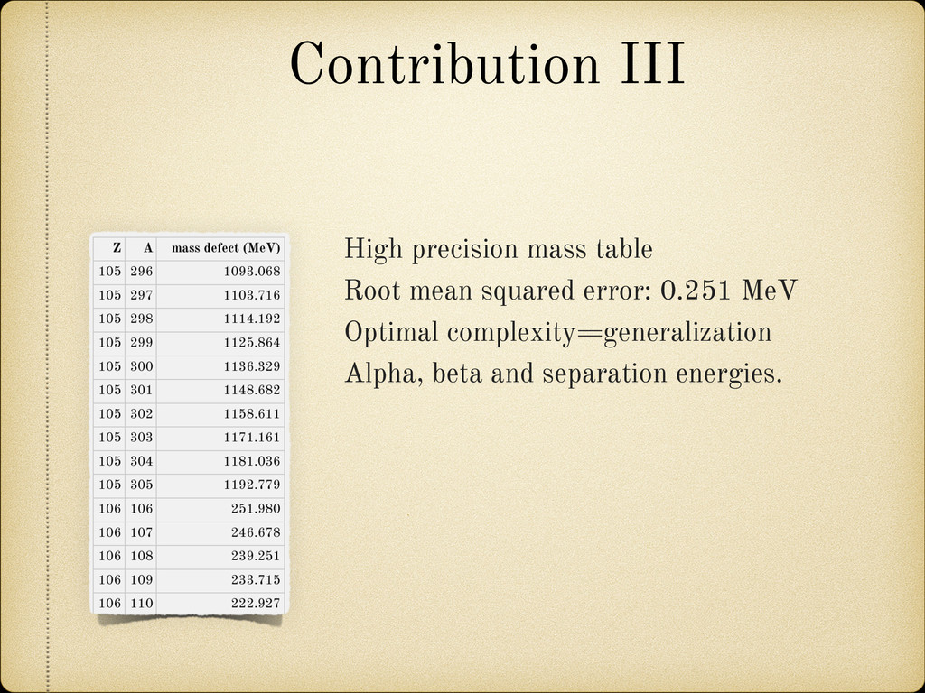
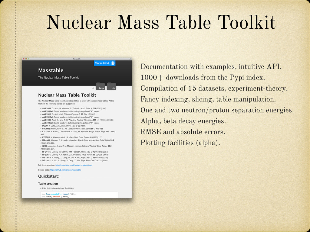
downloads from the Pypi index. Compilation of 15 datasets, experiment-theory. Fancy indexing, slicing, table manipulation. One and two neutron/proton separation energies. Alpha, beta decay energies. RMSE and absolute errors. Plotting facilities (alpha).
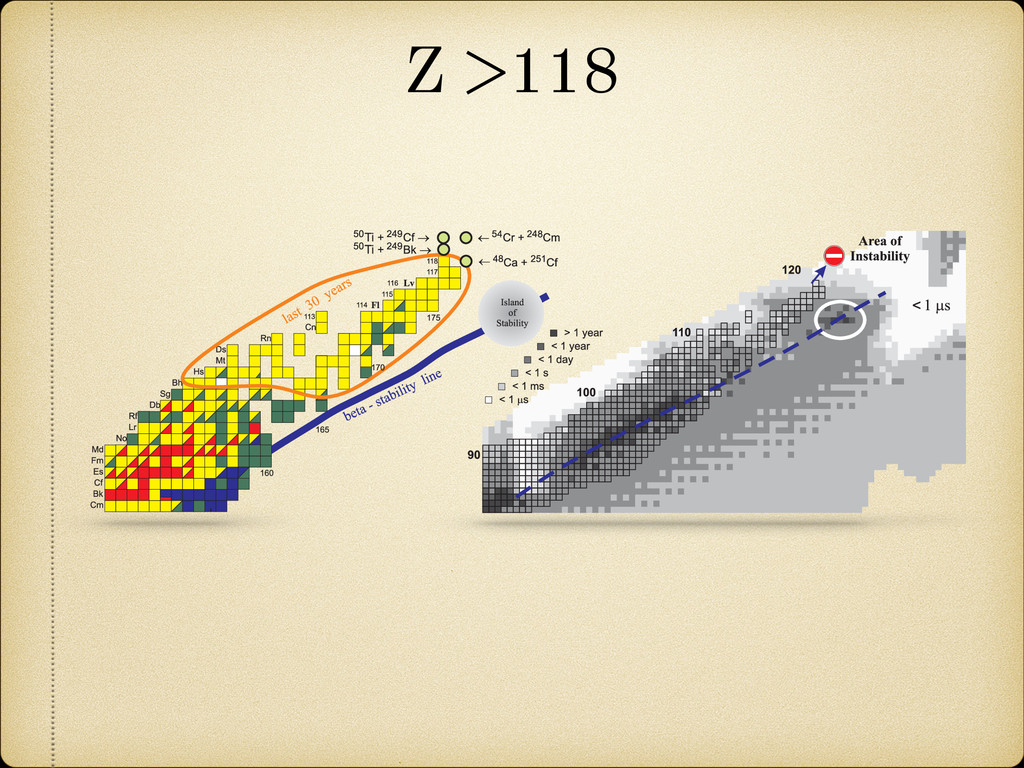
toward the neutron axis, in fusion reactions of stable nuclei one may produce only proton rich isotopes of heavy elements. That is the main reason for the impossibility to reach the center of the “island of stability” (Z ∼ 110 ÷ 120 and N ∼ 184) in fusion reactions with stable projectiles. Note that for elements with Z > 100 only neutron deficient isotopes (located to the left of the stability line) have been synthesized so far (see the left panel of Fig. 1). Figure 1. (Left panel) Upper part of the nuclear map. Current and planned experiments on synthesis of elements 118-120 are shown. (Right panel) Predicted half-lives of SH nuclei and the “area of instability”. Known nuclei are shown by the outlined rectangles. Further progress in the synthesis of new elements with Z > 118 is not quite evident. Cross sections of the “cold” fusion reactions decrease very fast with increasing charge of the projectile. (they become less than 1 pb already for Z ≥ 112 [1, 2]). For the more asymmetric 48Ca induced fusion reactions rather constant values (of a few picobarns) of the cross sections for the >
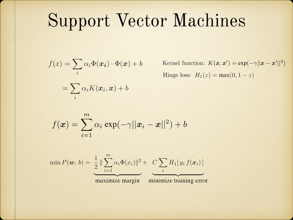
= exp(−γ||x − x′||2) is one of the most opular kernel functions. It adds a ”bump” around each data point: f(x) = m i=1 αi exp(−γ||xi − x||2) + b Φ Support Vector Machines - kernel trick II n rewrite all the SVM equations we saw before, but with the m i=1 αi Φ(xi ) equation: ecision function: f(x) = i αi Φ(xi ) · Φ(x) + b = i αiK(xi, x) + b ual formulation: min P(w, b) = 1 2 ∥ m i=1 αi Φ(xi )∥2 maximize margin + C i H1 [ yi f(xi ) ] minimize training error 28 RBF-SVMs The RBF kernel K(x, x′) = exp(−γ||x − x′||2) is o popular kernel functions. It adds a ”bump” around ea f(x) = m i=1 αi exp(−γ||xi − x||2) Φ . . Φ(x) Φ(x') x x' Using this one can get state-of-the-art results. 25 Support Vector Machines - kernel trick II We can rewrite all the SVM equations we saw before, but with the w = m i=1 αi Φ(xi ) equation: • Decision function: f(x) = i αi Φ(xi ) · Φ(x) + b = i αiK(xi, x) + b • Dual formulation: min P(w, b) = 1 2 ∥ m i=1 αi Φ(xi )∥2 maximize margin + C i H1 [ yi f(xi ) ] minimize training error Kernel function: • Primal formulation: min P(w, b) = 1 2 ∥w∥2 maximize margin + C i H minimize Ideally H1 would count the number of errors, appro Hinge Loss H1 (z) = max(0, 1 − z) 0 1 H (z) Hinge loss:
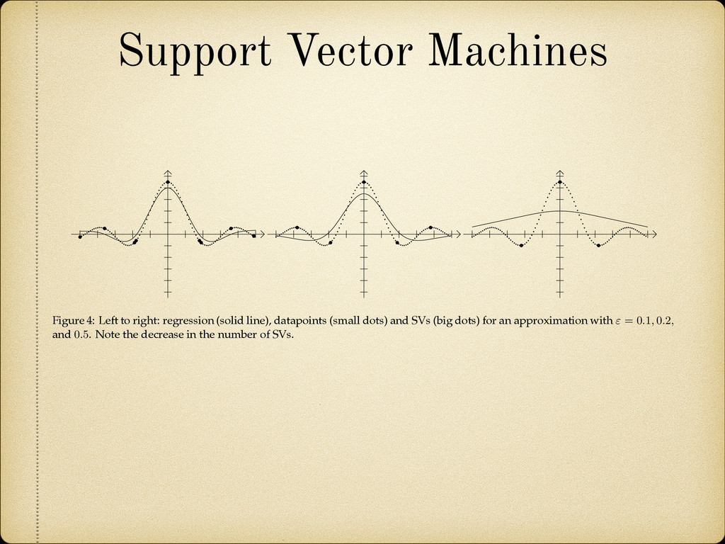
0.4 0.6 -1 -0.8 -0.6 -0.4 -0.2 0 0.2 0.4 0.6 0.8 1 -1 -0.8 -0.6 -0.4 -0.2 0 0.2 0.4 0.6 -1 -0.8 -0.6 -0.4 -0.2 0 0.2 0.4 0.6 0.8 1 -1 -0.8 -0.6 -0.4 -0.2 0 0.2 0.4 0.6 -1 -0.8 -0.6 -0.4 -0.2 0 0.2 0.4 0.6 0.8 1 Figure 3: Left to right: approximation of the function sinc x with precisions ε = 0.1, 0.2, and 0.5. The solid top and the bottom lines indicate the size of the ε–tube, the dotted line in between is the regression. Figure 4: Left to right: regression (solid line), datapoints (small dots) and SVs (big dots) for an approximation with ε = 0.1, 0.2, and 0.5. Note the decrease in the number of SVs. 5 Optimization Algorithms While there has been a large number of implementations of SV algorithms in the past years, we focus on a few algorithms which will be presented in greater detail. This selection is somewhat biased, as it contains these algorithms the authors are most familiar with. However, we think that this overview contains some of the most effective ones and will be useful for practitioners who would like to actually code a SV machine by themselves. But before doing so we will briefly cover ma- jor optimization packages and strategies. 5.1 Implementations proximations are close enough together, the second sub- algorithm, which permits a quadratic objective and con- verges very rapidly from a good starting value, is used. Recently an interior point algorithm was added to the software suite. CPLEX by CPLEX Optimization Inc. [1994] uses a primal- dual logarithmic barrier algorithm [Megiddo, 1989] in- stead with predictor-corrector step (see eg. [Lustig et al., 1992, Mehrotra and Sun, 1992]). MINOS by the Stanford Optimization Laboratory [Murtagh and Saunders, 1983] uses a reduced gradient algorithm in conjunction with a quasi-Newton algorithm. The con-
![mass excess compared to experimental results from Audi 2012 [2]](https://files.speakerdeck.com/presentations/be6e34107af70131588b1e6022973ecb/slide_51.jpg)
![Half lives Well before the discovery in 1928 [121] that](https://files.speakerdeck.com/presentations/be6e34107af70131588b1e6022973ecb/slide_53.jpg)