Travelling Salesman in Python

Transcript

1. Travelling Salesman
   in Python
   Rory Hart
   @falican
   

   View Slide

2. The Travelling Salesman Problem
   Given a list of cities and the distances between
   each pair of cities, what is the shortest possible
   route that visits each city exactly once and
   returns to the origin city?
   

   View Slide

3. Applications
   ● Planning
   ● Logistics
   ● Microchips
   ● DNA
   

   View Slide

4. Brute Force
   Approximately O(n!) where n is the number of
   cities.
   4! = 24
   8! = 40320
   16! = 20922789888000
   Oh no! Lets not bother with that.
   

   View Slide

5. Some better approaches?
   

   View Slide

6. A Greedy Algorithm
   From the first city travel to closest city. Keep
   repeating, traveling to the nearest unvisited
   city.
   Also known as Nearest Neighbour (NN).
   

   View Slide

7. Simple to Implement
   def nearest_tour(distances, count):
   available = range(1, count)
   tour = [0]
   while available:
   nearest = numpy.argmin(distances[tour[-1]][available])
   tour.append(available.pop(nearest))
   solution = numpy.array(tour, dtype=numpy.int)
   cost = calc_cost(solution, distances)
   return solution, cost
   

   View Slide

8. Simple to Implement
   def nearest_tour(distances, count):
   available = range(1, count)
   tour = [0]
   while available:
   nearest = numpy.argmin(distances[tour[-1]][available])
   tour.append(available.pop(nearest))
   solution = numpy.array(tour, dtype=numpy.int)
   cost = calc_cost(solution, distances)
   return solution, cost
   

   View Slide

9. With Some NumPy/SciPy
   def calc_distances(coords):
   return numpy.rint(
   scipy.spatial.distance.squareform(
   scipy.spatial.distance.pdist(coords, 'euclidean')))
   def calc_cost(solution, distances):
   cost = distances[solution[:-1], solution[1:]].sum()
   cost += distances[solution[-1], solution[0]]
   return cost
   

   View Slide

10. Demo
    

    View Slide

11. Local Search
    1. Make a small change.
    2. Check if the change is better.
    3. If better keep the solution, otherwise revert.
    

    View Slide

12. 2-opt: A local search heuristic
    

    View Slide

13. Not too complex
    def two_opt(solution, cost, count, calc_cost):
    best_cost = cost = calc_cost(solution)
    improving = True
    while improving:
    improving = False
    for i in xrange(1, count-2):
    for j in xrange(i+1, count):
    solution[i:j+1] = solution[j-count:i-count-1:-1]
    cost = calc_cost(solution)
    if cost < best_cost:
    best_cost = cost
    improving = True
    else:
    solution[i:j+1] = solution[j-count:i-count-1:-1]
    return solution, cost
    

    View Slide

14. Not too complex, thanks NumPy
    def two_opt(solution, cost, count, calc_cost):
    best_cost = cost = calc_cost(solution)
    improving = True
    while improving:
    improving = False
    for i in xrange(1, count-2):
    for j in xrange(i+1, count):
    solution[i:j+1] = solution[j-count:i-count-1:-1]
    cost = calc_cost(solution)
    if cost < best_cost:
    best_cost = cost
    improving = True
    else:
    solution[i:j+1] = solution[j-count:i-count-1:-1]
    return solution, cost
    

    View Slide

15. Demo
    

    View Slide

16. Local Search Issues
    ● Gets stuck in at a local minimum.
    ● Cannot prove a solution is the optimum.
    

    View Slide

17. Meta-heuristics
    

    View Slide

18. Guided Local Search (GLS)
    Each time we reach a local minimum penalise
    the edges that have the maximum utility. Then
    used these penalties in a modified cost
    function.
    

    View Slide

19. Utility Function and the Penalties
    def penalise(solution):
    sol_dists = distances[solution[0:-1], solution[1:]]
    sol_dists = numpy.append(sol_dists, (distances[solution[0], solution[-1]],))
    sol_pens = penalties[solution[0:-1], solution[1:]]
    sol_pens = numpy.append(sol_pens, (penalties[solution[0], solution[-1]],))
    utility = sol_dists/(sol_pens+1)
    index_a = numpy.argmax(utility)
    index_b = index_a+1 if index_a != count-1 else 0
    a = solution[index_a]
    b = solution[index_b]
    penalties[a,b] += 1.0
    penalties[b,a] += 1.0
    

    View Slide

20. Cost Function with Penalties
    def gls_calc_cost(solution, distances, penalties, best_cost):
    cost = calc_cost(solution, distances)
    sol_pens = penalties[solution[:-1], solution[1:]]
    gls_cost = (
    cost +
    LAMBDA* # lambda (generally 0.2 to 0.3 for TSP)
    (best_cost/count+1) * # alpha
    (sol_pens.sum() + penalties[solution[-1], solution[0]]))
    return gls_cost
    

    View Slide

21. Search function
    while 1:
    solution, gls_cost = two_opt(
    solution, gls_cost, len(distances), gls_calc_cost,
    redraw_guess)
    cost = calc_cost(solution, distances)
    if cost < best_cost:
    best_cost = cost
    best_solution[:] = solution
    penalise(solution)
    

    View Slide

22. Demo
    

    View Slide

23. Guided Local Search Issues
    ● Still cannot prove a solution is the optimum.
    ● Will never terminate.
    

    View Slide

24. Resources
    Demo source https://github.com/hartror/gls_tsp
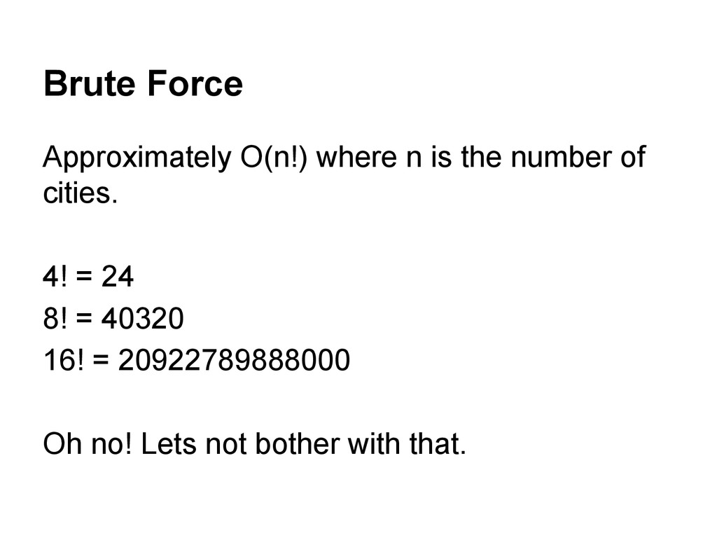
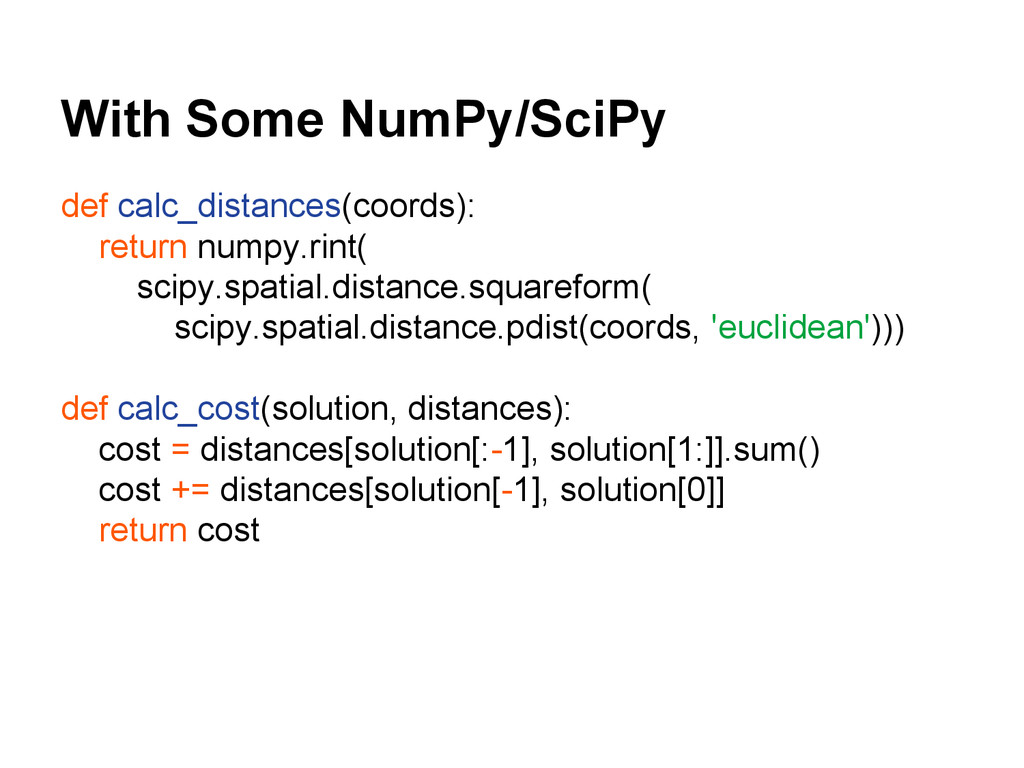
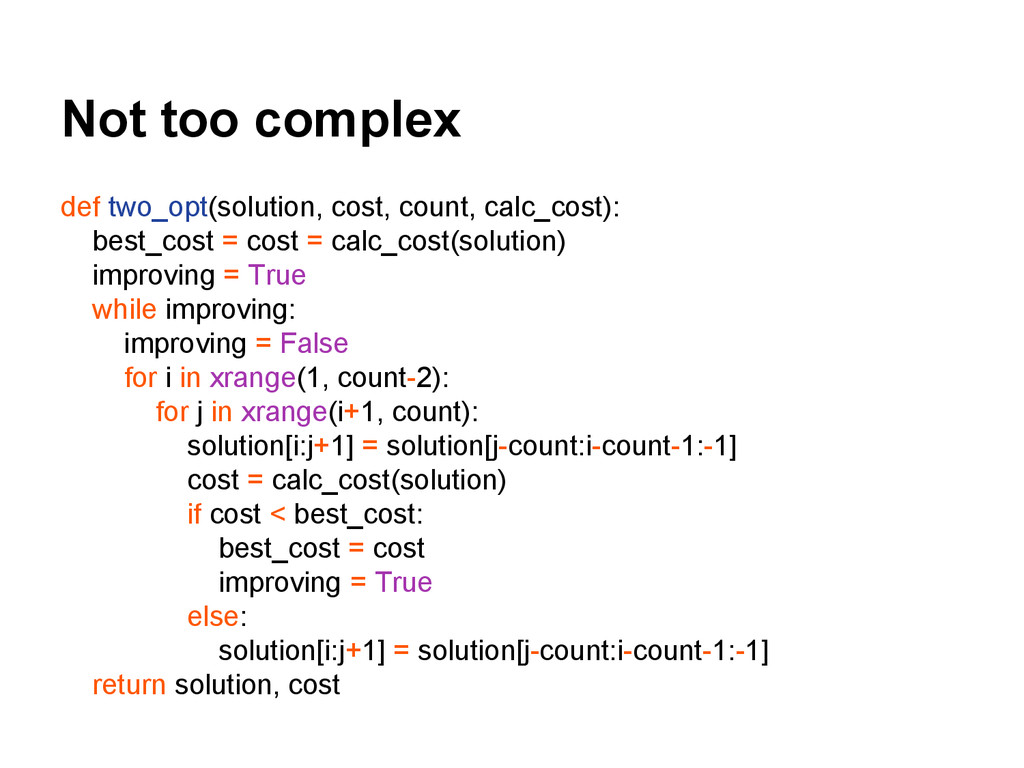
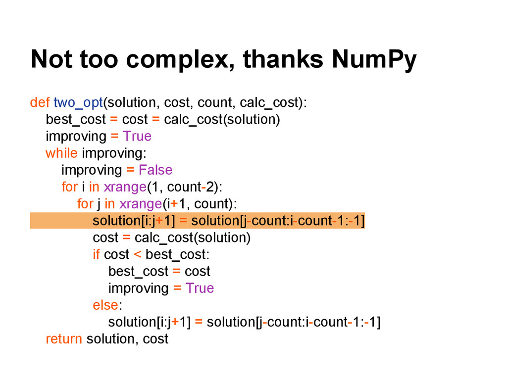
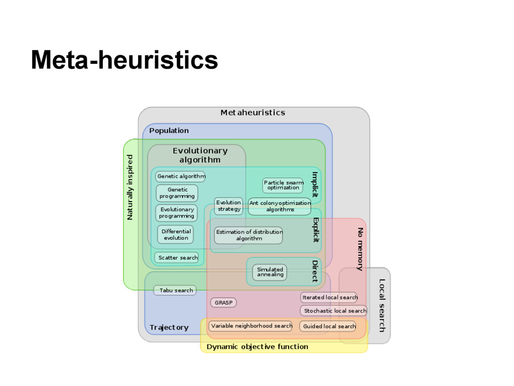
    Christos Voudouris, Edward Tsang, Guided local search
    and its application to the traveling salesman problem,
    European Journal of Operational Research 113 (1999) 469-
    499
    http://www.ceet.niu.
    edu/faculty/ghrayeb/IENG576s04/papers/Local%
    20Search/local%20search%20for%20tsp.pdf
    TSP Problem Library http://comopt.ifi.uni-heidelberg.
    de/software/TSPLIB95/
    

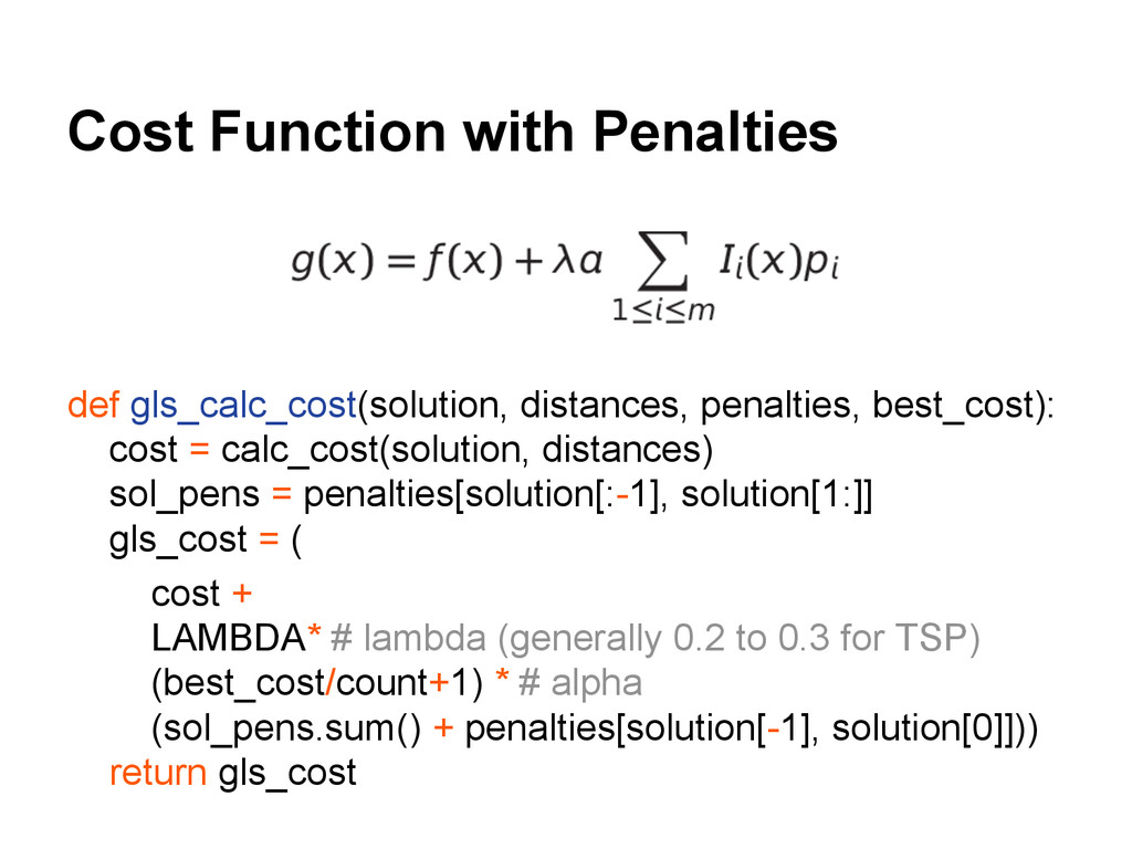
    View Slide