Uniform asymptotic approximation of diffusion to a small target

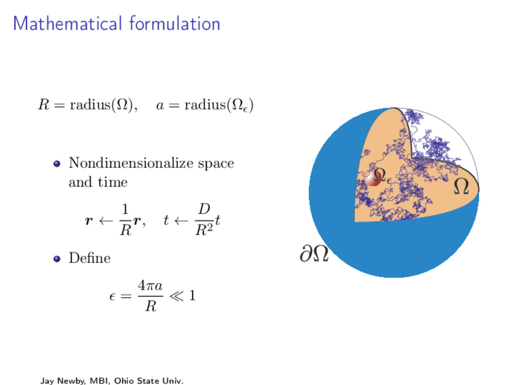
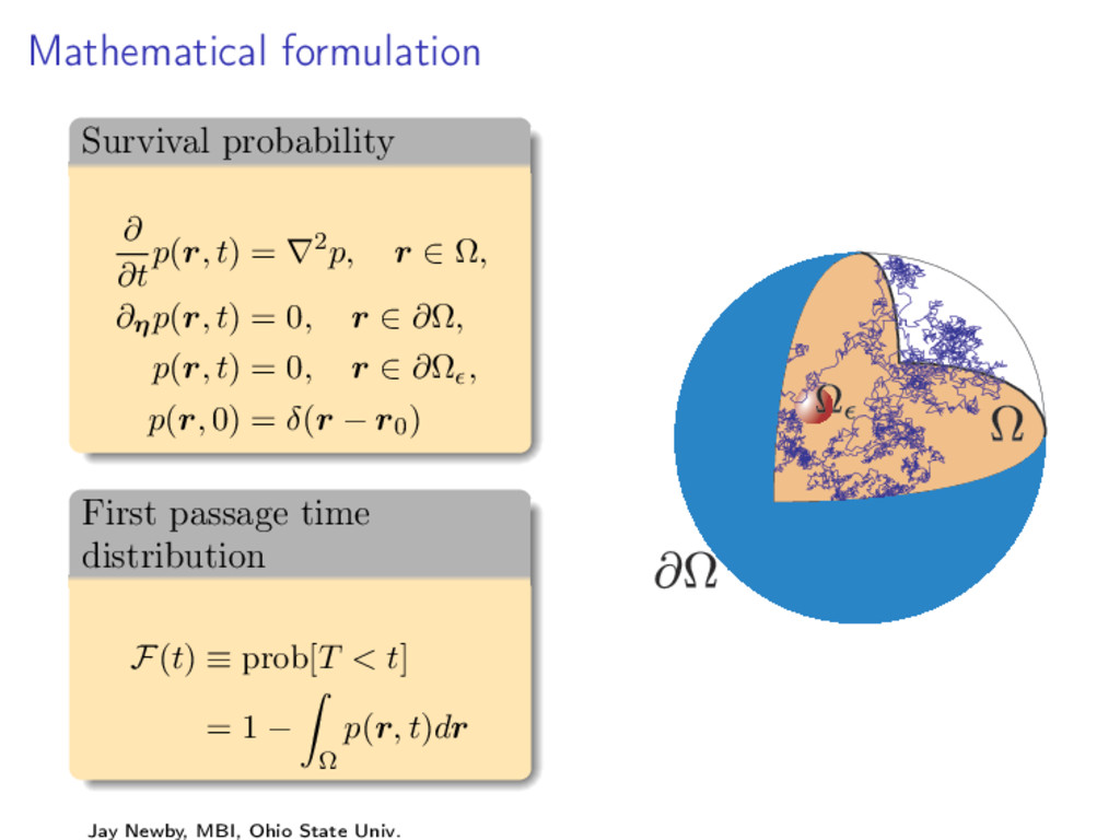
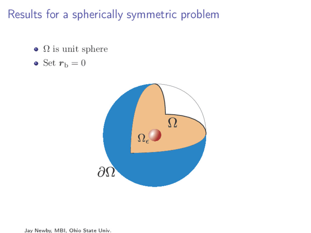
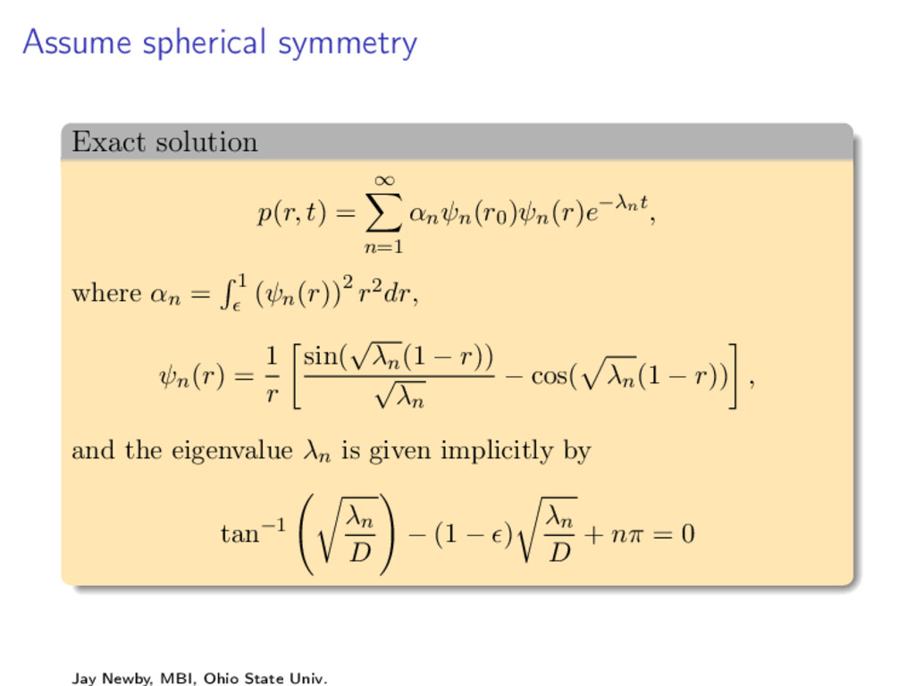
The problem of the time required for a diffusing molecule, within a large bounded domain, to first locate a small target is prevalent in biological modeling. Here we study this problem for a small spherical target. We develop uniform in time asymptotic expansions in the target radius of the solution to the corresponding diffusion equation. Our approach is based on combining expansions of a long-time approximation of the solution, involving the first eigenvalue and eigenfunction of the Laplacian, with expansions of a short-time correction calculated by a pseudopotential approximation. These expansions allow the calculation of corresponding expansions of the first passage time density for the diffusing molecule to find the target. We demonstrate the accuracy of our method in approximating the first passage time density and related statistics for the spherically symmetric problem where the domain is a large concentric sphere about a small target centered at the origin.

Transcript

1. Uniform asymptotic approximation of diffusion to a small target Jay Newby in collaboration with Sam Isaacson, Boston University Mathematical Bioscience Institute, Ohio State University, USA Jay Newby, MBI, Ohio State Univ.
2. Transport in complex cellular geometries Jay Newby, MBI, Ohio State Univ.
3. Mathematical formulation R = radius(Ω), a = radius(Ω ) Nondimensionalize space and time r ← 1 R r, t ← D R2 t Define = 4πa R 1 Jay Newby, MBI, Ohio State Univ.
4. Mathematical formulation Survival probability ∂ ∂t p(r, t) = ∇2p, r ∈ Ω, ∂ηp(r, t) = 0, r ∈ ∂Ω, p(r, t) = 0, r ∈ ∂Ω , p(r, 0) = δ(r − r0) First passage time distribution F(t) ≡ prob[T < t] = 1 − Ω p(r, t)dr Jay Newby, MBI, Ohio State Univ.
5. Replace Dirichlet boundary with source term? Work with Laplace transform ˜ p(r, s) = ∞ 0 e−stp(r, t)dt Dirichlet problem −∇2 ˜ p + s˜ p = δ(r − r0), ∂η ˜ p(r, s) = 0, r ∈ ∂Ω, ˜ p(r, s) = 0, r ∈ ∂Ω , Source term −∇2 ˜ p + s˜ p = δ(r − r0) + k˜ p(r, s)δ(r − rb), ∂η ˜ p(r, s) = 0, r ∈ ∂Ω, Jay Newby, MBI, Ohio State Univ.
6. Replace Dirichlet boundary with source term? Source term −∇2 ˜ p + s˜ p = δ(r − r0) + k˜ pδ(r − rb), ∂η ˜ p(r, s) = 0, r ∈ ∂Ω, Green’s function (solution to = 0 problem) −∇2 ˜ G + s ˜ G = δ(r − r ), ∂η ˜ G(r, r ) = 0, r ∈ ∂Ω Solution satisfies ˜ p(r, s) = ˜ G(r, r0) + k˜ p(rb, s) ˜ G(r, rb) Jay Newby, MBI, Ohio State Univ.
7. Replace Dirichlet boundary with source term? Take limit r → rb ˜ p(rb, s) = ˜ G(rb, r0) + k˜ p(rb, s) ˜ G(rb, rb) ⇒ ˜ p(rb, s) = ˜ G(rb, r0) 1 − k ˜ G(rb, rb) Works fine in 1D, but for higher dimensions lim r→rb ˜ G(r, rb) → ∞ In 3D ˜ G(r, rb) ∼ 1 4π |r − rb| , r → rb Jay Newby, MBI, Ohio State Univ.
8. Long-time asymptotic approximation Cheviakov, A. and Ward, M. J., Optimizing the principal eigenvalue of the Laplacian in a sphere with interior traps, Math. Computer Modelling, 53 (2011), pp. 1394-1409. General theory Ward, M. J. and Keller, J. B. SIAM J. Appl. Math, 53:3, 770-798, (1993) Condamin, S. and Bénichou, O. and Moreau, M. Phys. Rev. E, 75:021111, (2007) Schuss, Z. and Singer, A. and Holcman, D. PNAS, 104:41, 16098-16103, (2007) Jay Newby, MBI, Ohio State Univ.
9. Long-time asymptotic approximation Eigenfunction expansion p(r, t) = ∞ j=0 ψj(r0)ψj(r)e−λjt Long-time behavior dominated by smallest eigenvalue p(r, t) ∼ ψ0(r0)ψ0(r)e−λ0t, λ1t 1 Perturbation expansion in p(r, t) ∼ 1 |Ω| e−4πD |Ω| t, 1, λ1t 1 Initial position is uniformly distributed p(r, 0) = 1 |Ω| = δ(r − r0) Jay Newby, MBI, Ohio State Univ.
10. Challenges for the long-time approximation Long time approximation F(t) ∼ 1 − e−4πD |Ω| t 1 no dependence on r0 2 one timescale: the mean T ∼ 1 λ0 ∼ |Ω| 4π D 3 not all statistics of the first passage time are well approximated Jay Newby, MBI, Ohio State Univ.
11. For example, the mode Defined as the most likely first passage time τm ≡ arg max t≥0 d dt F(t) For an exponential RV, the mode is τm = 0 We should then expect that τm → 0 as → 0 Jay Newby, MBI, Ohio State Univ.
12. Approach Split solution into two parts: long time and short time p(r, t) = pLT (r, t) + pST (r, t) modified initial condition pLT (r, 0) = ψ(r), δ(r − r0) ψ(r) = ψ(r0)ψ(r) pST (r, 0) = δ(r − r0) − ψ(r0)ψ(r) The plan 1 Use well known large time approximation 2 Use pseudopotential operator for short time problem Jay Newby, MBI, Ohio State Univ.
13. Short time problem Define r = |r − rb| Pseudopotential operator − ∂ ∂r [rpST (r, t)] δ(r − rb) Pseudopotential is a way of replacing Dirichlet BC on ∂Ω with source term Jay Newby, MBI, Ohio State Univ.
14. Short time problem Pseudopotential problem ∂pST ∂t = ∇2pST − ∂ ∂r [rpST (r, t)] δ(r − rb) ∂ηpST (r, t) = 0, r ∈ ∂Ω pST (r, 0) = δ(r − r0) − ψ(r0)ψ(r) Split pST (r, t) into - regular part φ(r, t) - singular part q(t) 4π|r−rb| pST (r, t) = φ(r, t) + q(t) 4π |r − rb| Assume φ(r, t) is bounded as r → rb Jay Newby, MBI, Ohio State Univ.
15. Short time problem Let G(r, r , t) be the fundamental solution to the diffusion equation on Ω Fundamental solution (solution to the = 0 problem) ∂ ∂t G(r, r , t) = ∇2G, r ∈ Ω, ∂ηG = 0, r ∈ ∂Ω, G(r, r , 0) = δ(r − r ) Note that ∞ 0 G(r, r , t) − 1 |Ω| dt = U(r, r ) Jay Newby, MBI, Ohio State Univ.
16. Short time problem Integral equation form φ(r, t) = − t 0 R(r, rb, t − s)φ(rb, s)ds + Ω G(r, r , t)φ(r , 0)dr where we write ˜ G(r, r , s) = ˜ R(r, r , s) + e−|r−r | √ s D 4π |r − r | Asymptotic expansion φ(r, t) ∼ φ(0)(r, t) + φ(1)(r, t) + φ(2)(r, t) 2 Jay Newby, MBI, Ohio State Univ.
17. First order result Survival density p(r, t) ∼ G(r, r0, t) − 1 |Ω| 1 − e−λt − |Ω| U(r, rb)e−λt − U(rb, r0)(1 − e−λt) + |Ω| Ω G(r, r , t)U(r , rb)dr − t 0 G(r, rb, t − s) G(rb, r0, s) − 1 |Ω| ds. First passage time distribution F(t) ∼ [1 − U(rb, r0)] 1 − e−λt + t 0 G(rb, r0, t) − 1 |Ω| ds Jay Newby, MBI, Ohio State Univ.
18. Results for a spherically symmetric problem Ω is unit sphere Set rb = 0 Jay Newby, MBI, Ohio State Univ.
19. Assume spherical symmetry Exact solution p(r, t) = ∞ n=1 αnψn(r0)ψn(r)e−λnt, where αn = 1 (ψn(r))2 r2dr, ψn(r) = 1 r sin( √ λn(1 − r)) √ λn − cos( λn(1 − r)) , and the eigenvalue λn is given implicitly by tan−1 λn D − (1 − ) λn D + nπ = 0 Jay Newby, MBI, Ohio State Univ.
20. 10−3 10−2 10−1 100 −2 0 2 4 6 8 10 12 14 r p t = 1.0 t = .1 t = 0.01 t = 0.001 Figure: The spatial density function p(r, t) (black curve) and its approximation: leading order (blue curve), first order (dashed curve). r0 = 0.8 and = 0.001 (similar to the width of measured DNA binding potentials). Jay Newby, MBI, Ohio State Univ.
21. 10-3 10-2 10-1 100 101 102 t 0.0 0.5 1.0 1.5 2.0 2.5 f long time first order second order exact 0 10 20 30 40 50 t 10-4 10-3 10-2 10-1 100 f Figure: The first passage time density, f(t), for r0 = 0.3 and = 0.05. First passage time density f(t) ≡ d dt F(t) Jay Newby, MBI, Ohio State Univ.
22. 10-3 10-2 10-1 100 101 102 t 0.00 0.05 0.10 0.15 0.20 f 0 10 20 30 40 50 t 10-4 10-3 10-2 10-1 100 f Figure: The first passage time density, f(t), for r0 = 0.8 and = 0.05. Jay Newby, MBI, Ohio State Univ.
23. 10-4 10-3 10-2 10-1 10-11 10-10 10-9 10-8 10-7 10-6 10-5 10-4 10-3 10-2 10-1 100 101 max norm error r0 =0.3 r0 =0.65 r0 =0.9 Figure: The long-time approximation (solid curves) and the second order uniform approximation (dashed curves). Jay Newby, MBI, Ohio State Univ.
24. 0.3 0.4 0.5 0.6 0.7 0.8 0.9 1.0 r0 0.0 0.1 0.2 0.3 0.4 0.5 mode =0.001 =0.01 =0.1 Figure: The mode (most likely binding time). The exact solution (solid curves), the first order approximation (dash dotted curves), and the 2nd order approximation (dashed curves). Jay Newby, MBI, Ohio State Univ.
25. Acknowledgments Collaborator: Sam Isaacson Jay Newby, MBI, Ohio State Univ.