An Introduction to Hidden Markov Models

A very short introduction on Hidden Markov Models.

Originally presented as a ShiftForward Tech Talk, a series of weekly talks presented by ShiftForward employees.

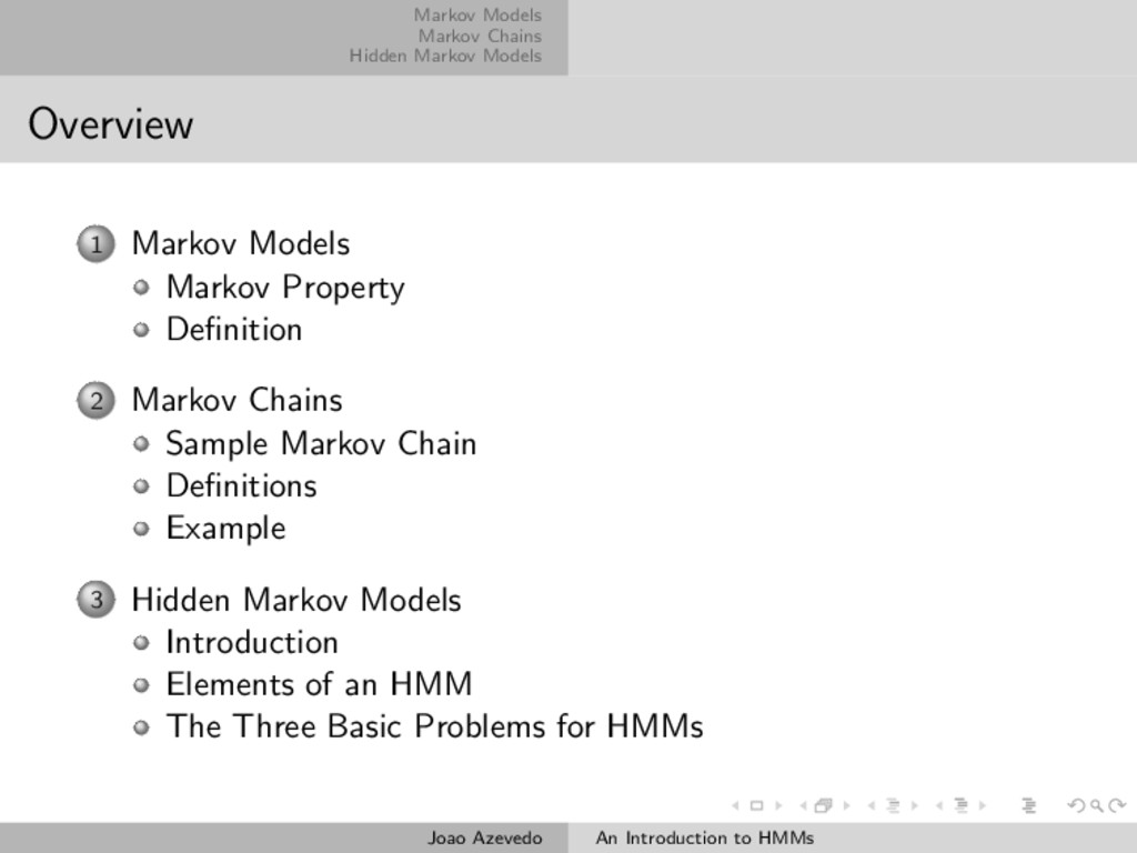
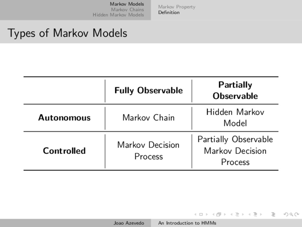
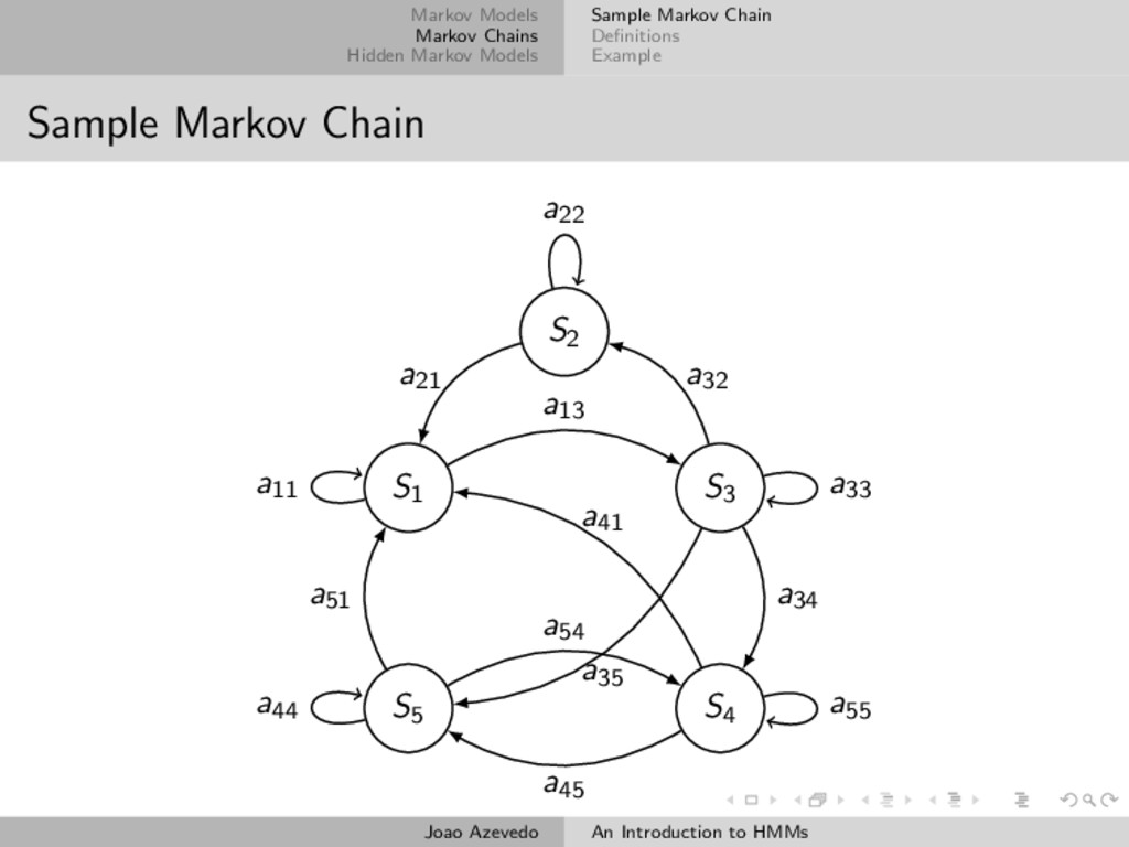
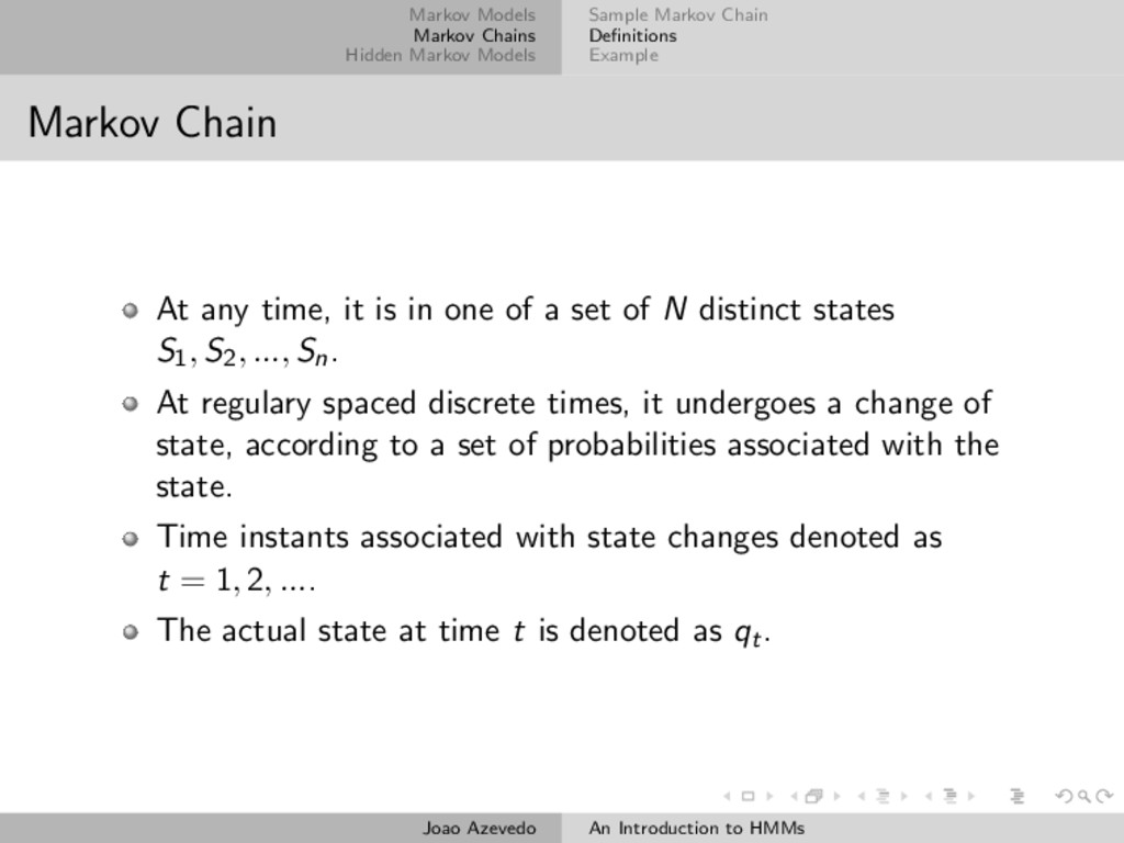
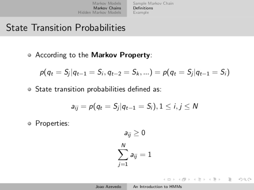
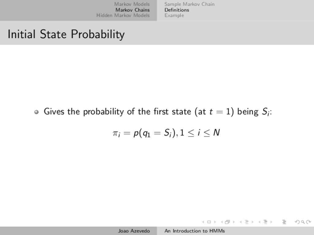
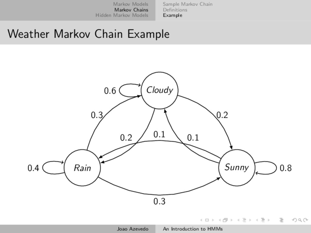
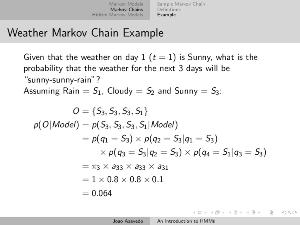
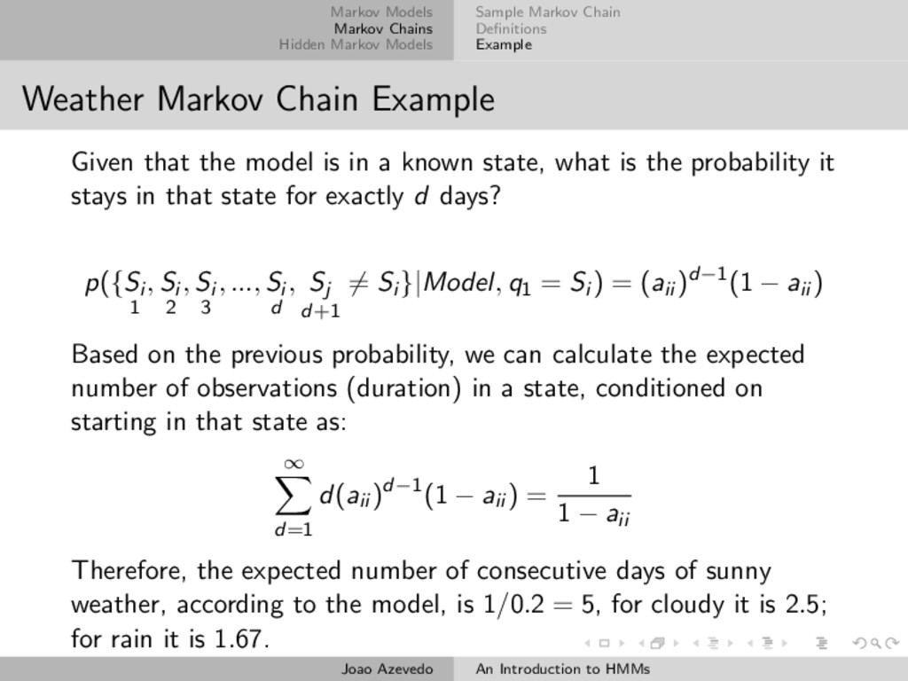
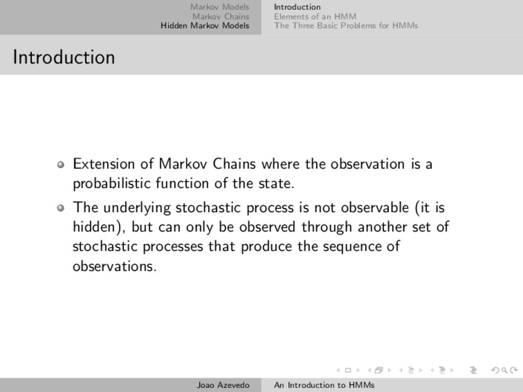
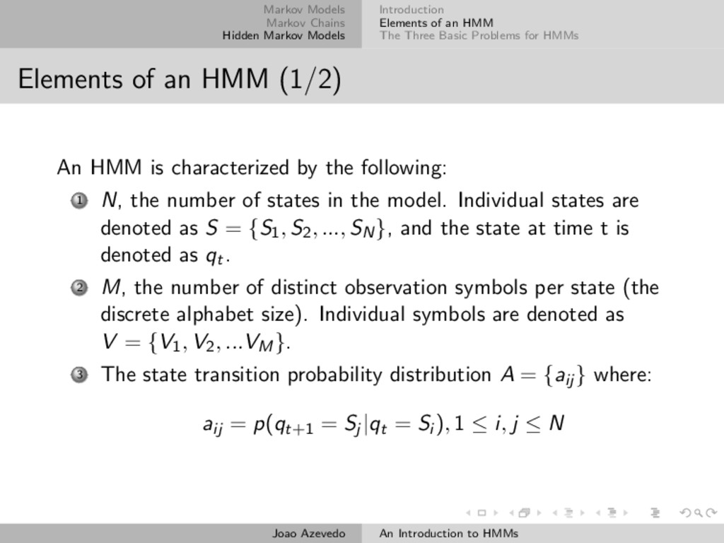
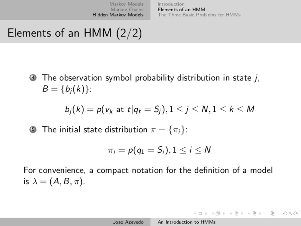
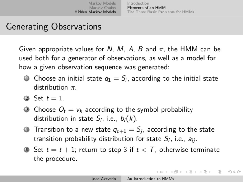
The talk starts by describing the Markov property as an introduction to Markov Models. Markov Chains are then presented, serving as the example of fully observable autonomous Markov Models. An example of a Weather Markov Chain illustrates some applications for the model. Markov Chains are then extended to Hidden Markov Models. The elements of an HMM are described, and the three basic problems of HMMs are introduced:

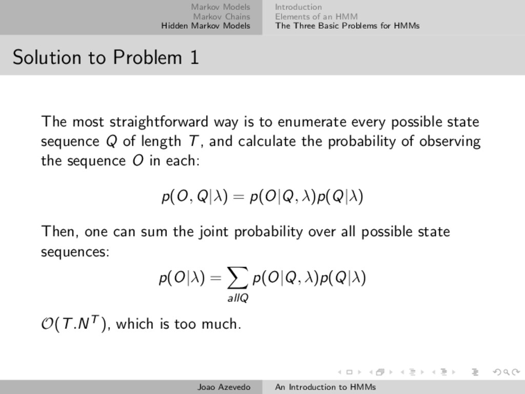
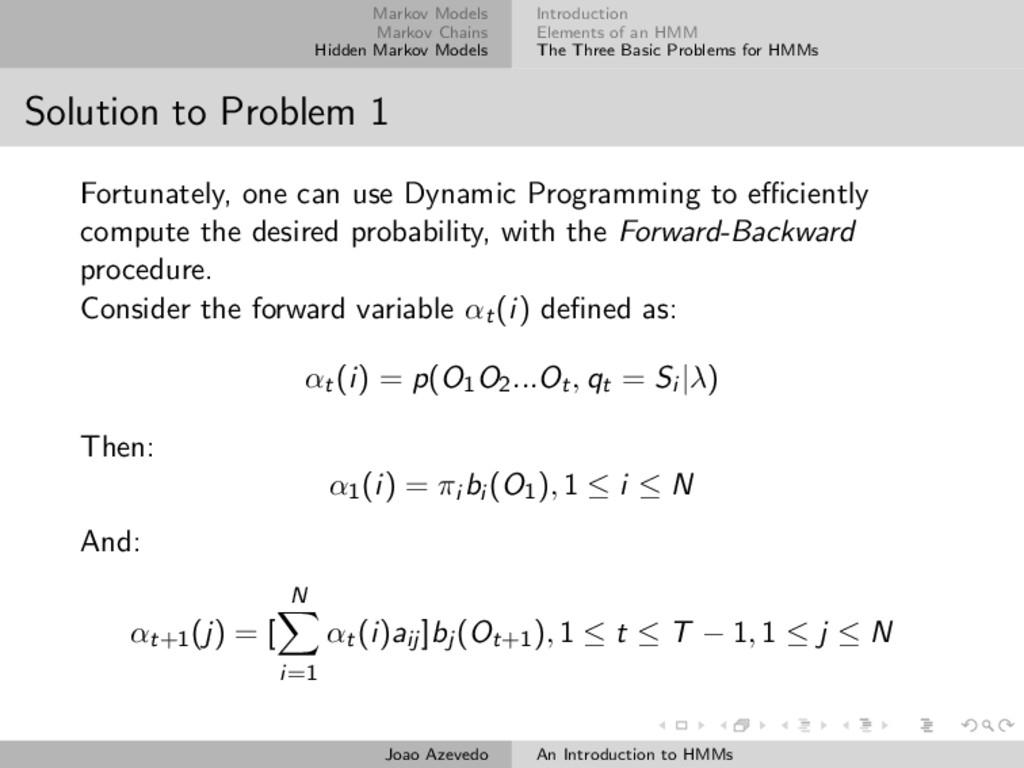
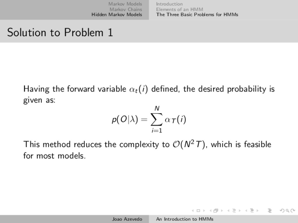
1. Determining the probability of a sequence of observations having been generated by a given model.
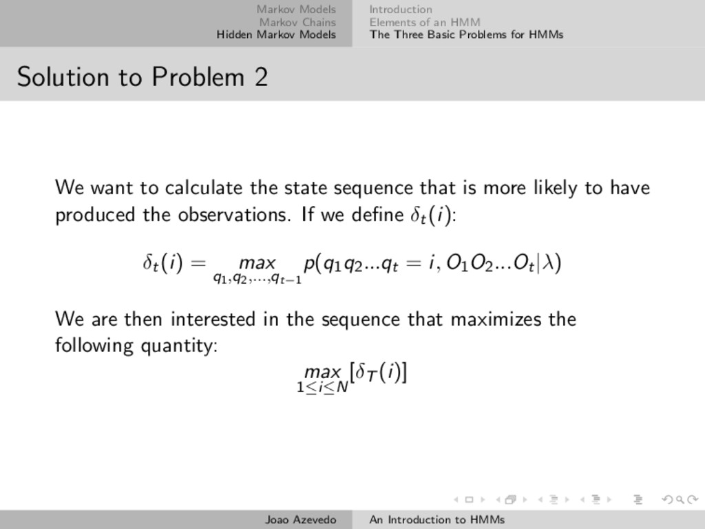
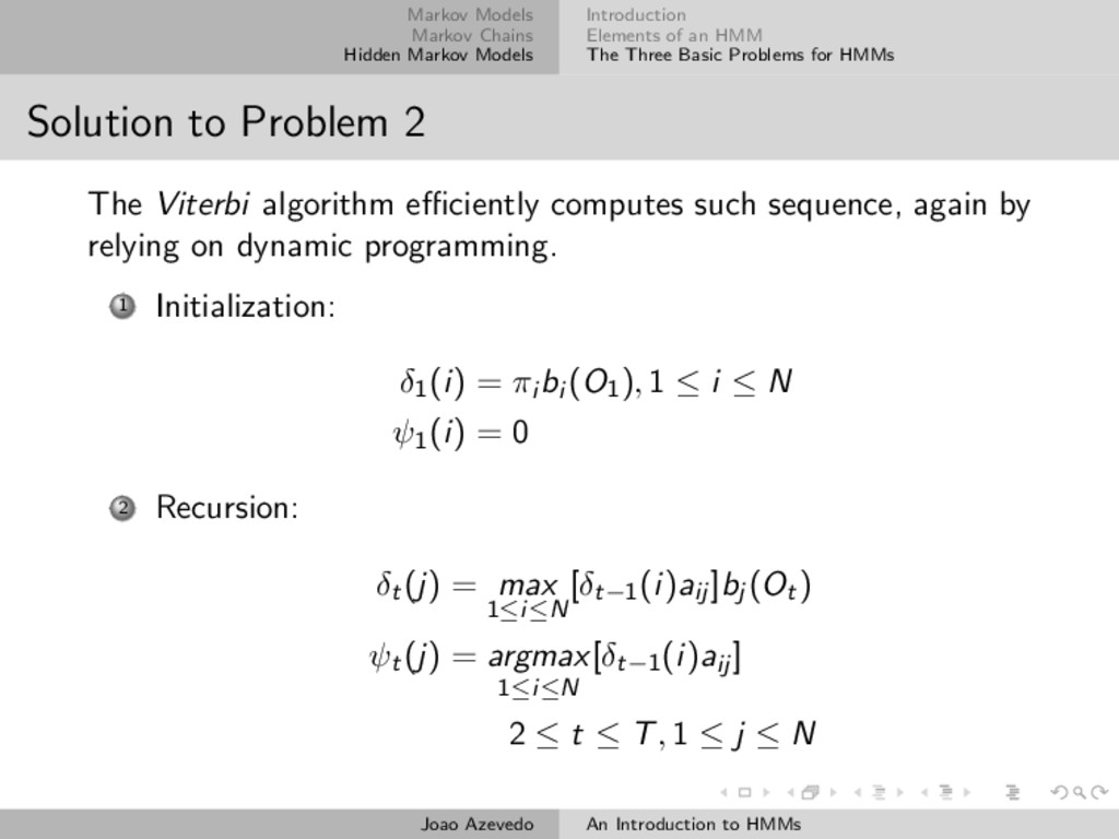
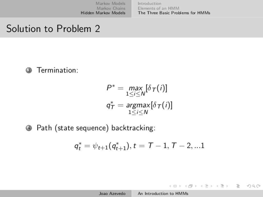
2. Determining the state sequence which best explains a sequence of observations.
3. Adjusting the model parameters in order to maximize the probability of generating a given sequence of observations.

Algorithms to solve the three problems are introduced, and some conclusions are drawn on the subject.

Transcript

1. Markov Models Markov Chains Hidden Markov Models An Introduction to Hidden Markov Models Joao Azevedo ShiftForward Tech Talks joao@shiftforward.eu June 26, 2015 Joao Azevedo An Introduction to HMMs
2. Markov Models Markov Chains Hidden Markov Models Overview 1 Markov Models Markov Property Definition 2 Markov Chains Sample Markov Chain Definitions Example 3 Hidden Markov Models Introduction Elements of an HMM The Three Basic Problems for HMMs Joao Azevedo An Introduction to HMMs
3. Markov Models Markov Chains Hidden Markov Models Markov Property Definition Markov Property The memoryless property of a stochastic process, i.e. the conditional probability distribution of future states of the process depends only upon the present state, not on the sequence of states that preceded it. Joao Azevedo An Introduction to HMMs
4. Markov Models Markov Chains Hidden Markov Models Markov Property Definition Markov Models Stochastic models used to model randomly changing systems following the Markov property. Joao Azevedo An Introduction to HMMs
5. Markov Models Markov Chains Hidden Markov Models Markov Property Definition Types of Markov Models Fully Observable Partially Observable Autonomous Markov Chain Hidden Markov Model Controlled Markov Decision Process Partially Observable Markov Decision Process Joao Azevedo An Introduction to HMMs
6. Markov Models Markov Chains Hidden Markov Models Sample Markov Chain Definitions Example Sample Markov Chain S1 S2 S3 S5 S4 a11 a13 a22 a33 a44 a55 a32 a21 a35 a34 a41 a54 a45 a51 Joao Azevedo An Introduction to HMMs
7. Markov Models Markov Chains Hidden Markov Models Sample Markov Chain Definitions Example Markov Chain At any time, it is in one of a set of N distinct states S1, S2, ..., Sn. At regulary spaced discrete times, it undergoes a change of state, according to a set of probabilities associated with the state. Time instants associated with state changes denoted as t = 1, 2, .... The actual state at time t is denoted as qt. Joao Azevedo An Introduction to HMMs
8. Markov Models Markov Chains Hidden Markov Models Sample Markov Chain Definitions Example State Transition Probabilities According to the Markov Property: p(qt = Sj |qt−1 = Si , qt−2 = Sk, ...) = p(qt = Sj |qt−1 = Si ) State transition probabilities defined as: aij = p(qt = Sj |qt−1 = Si ), 1 ≤ i, j ≤ N Properties: aij ≥ 0 N j=1 aij = 1 Joao Azevedo An Introduction to HMMs
9. Markov Models Markov Chains Hidden Markov Models Sample Markov Chain Definitions Example Initial State Probability Gives the probability of the first state (at t = 1) being Si : πi = p(q1 = Si ), 1 ≤ i ≤ N Joao Azevedo An Introduction to HMMs
10. Markov Models Markov Chains Hidden Markov Models Sample Markov Chain Definitions Example Weather Markov Chain Example Rain Cloudy Sunny 0.4 0.6 0.8 0.3 0.3 0.2 0.2 0.1 0.1 Joao Azevedo An Introduction to HMMs
11. Markov Models Markov Chains Hidden Markov Models Sample Markov Chain Definitions Example Weather Markov Chain Example Given that the weather on day 1 (t = 1) is Sunny, what is the probability that the weather for the next 3 days will be “sunny-sunny-rain”? Assuming Rain = S1, Cloudy = S2 and Sunny = S3: O = {S3, S3, S3, S1} p(O|Model) = p(S3, S3, S3, S1|Model) = p(q1 = S3) × p(q2 = S3|q1 = S3) × p(q3 = S3|q2 = S3) × p(q4 = S1|q3 = S3) = π3 × a33 × a33 × a31 = 1 × 0.8 × 0.8 × 0.1 = 0.064 Joao Azevedo An Introduction to HMMs
12. Markov Models Markov Chains Hidden Markov Models Sample Markov Chain Definitions Example Weather Markov Chain Example Given that the model is in a known state, what is the probability it stays in that state for exactly d days? p({Si 1 , Si 2 , Si 3 , ..., Si d , Sj d+1 = Si }|Model, q1 = Si ) = (aii )d−1(1 − aii ) Based on the previous probability, we can calculate the expected number of observations (duration) in a state, conditioned on starting in that state as: ∞ d=1 d(aii )d−1(1 − aii ) = 1 1 − aii Therefore, the expected number of consecutive days of sunny weather, according to the model, is 1/0.2 = 5, for cloudy it is 2.5; for rain it is 1.67. Joao Azevedo An Introduction to HMMs
13. Markov Models Markov Chains Hidden Markov Models Introduction Elements of an HMM The Three Basic Problems for HMMs Introduction Extension of Markov Chains where the observation is a probabilistic function of the state. The underlying stochastic process is not observable (it is hidden), but can only be observed through another set of stochastic processes that produce the sequence of observations. Joao Azevedo An Introduction to HMMs
14. Markov Models Markov Chains Hidden Markov Models Introduction Elements of an HMM The Three Basic Problems for HMMs Examples Coin toss with a curtain: On one side of a curtain, someone is performing a coin (or multiple coin) tossing experiment, telling you only the result of each coin flip. Urn and balls: A genie is in a room, and, according to some random process, chooses an urn from a set of N available ones. Each urn has a given amount of balls and you know there are M distinct colors for the balls. The genie picks a ball at random from the selected urn, tells you its color and chooses another urn according to the same random process. Joao Azevedo An Introduction to HMMs
15. Markov Models Markov Chains Hidden Markov Models Introduction Elements of an HMM The Three Basic Problems for HMMs Elements of an HMM (1/2) An HMM is characterized by the following: 1 N, the number of states in the model. Individual states are denoted as S = {S1, S2, ..., SN}, and the state at time t is denoted as qt. 2 M, the number of distinct observation symbols per state (the discrete alphabet size). Individual symbols are denoted as V = {V1, V2, ...VM}. 3 The state transition probability distribution A = {aij } where: aij = p(qt+1 = Sj |qt = Si ), 1 ≤ i, j ≤ N Joao Azevedo An Introduction to HMMs
16. Markov Models Markov Chains Hidden Markov Models Introduction Elements of an HMM The Three Basic Problems for HMMs Elements of an HMM (2/2) 4 The observation symbol probability distribution in state j, B = {bj (k)}: bj (k) = p(vk at t|qt = Sj ), 1 ≤ j ≤ N, 1 ≤ k ≤ M 5 The initial state distribution π = {πi }: πi = p(q1 = Si ), 1 ≤ i ≤ N For convenience, a compact notation for the definition of a model is λ = (A, B, π). Joao Azevedo An Introduction to HMMs
17. Markov Models Markov Chains Hidden Markov Models Introduction Elements of an HMM The Three Basic Problems for HMMs Generating Observations Given appropriate values for N, M, A, B and π, the HMM can be used both for a generator of observations, as well as a model for how a given observation sequence was generated: 1 Choose an initial state q1 = Si , according to the initial state distribution π. 2 Set t = 1. 3 Choose Ot = vk according to the symbol probability distribution in state Si , i.e., bi (k). 4 Transition to a new state qt+1 = Sj , according to the state transition probability distribution for state Si , i.e., aij . 5 Set t = t + 1; return to step 3 if t < T, otherwise terminate the procedure. Joao Azevedo An Introduction to HMMs
18. Markov Models Markov Chains Hidden Markov Models Introduction Elements of an HMM The Three Basic Problems for HMMs The Three Basic Problems for HMMs 1 Given the observation sequence O = O1O2...OT , and a model λ = (A, B, π), how do we efficiently compute p(O|λ)? 2 Given the observation sequence O = O1O2...OT , and the model λ, how do we choose a corresponding state sequence Q = q1q2...qT , which best explains the observations? 3 How do we adjust the model parameters λ = (A, B, π) to maximize p(O|λ). Joao Azevedo An Introduction to HMMs
19. Markov Models Markov Chains Hidden Markov Models Introduction Elements of an HMM The Three Basic Problems for HMMs Solution to Problem 1 The most straightforward way is to enumerate every possible state sequence Q of length T, and calculate the probability of observing the sequence O in each: p(O, Q|λ) = p(O|Q, λ)p(Q|λ) Then, one can sum the joint probability over all possible state sequences: p(O|λ) = allQ p(O|Q, λ)p(Q|λ) O(T.NT ), which is too much. Joao Azevedo An Introduction to HMMs
20. Markov Models Markov Chains Hidden Markov Models Introduction Elements of an HMM The Three Basic Problems for HMMs Solution to Problem 1 Fortunately, one can use Dynamic Programming to efficiently compute the desired probability, with the Forward-Backward procedure. Consider the forward variable αt(i) defined as: αt(i) = p(O1O2...Ot, qt = Si |λ) Then: α1(i) = πi bi (O1), 1 ≤ i ≤ N And: αt+1(j) = [ N i=1 αt(i)aij ]bj (Ot+1), 1 ≤ t ≤ T − 1, 1 ≤ j ≤ N Joao Azevedo An Introduction to HMMs
21. Markov Models Markov Chains Hidden Markov Models Introduction Elements of an HMM The Three Basic Problems for HMMs Solution to Problem 1 Having the forward variable αt(i) defined, the desired probability is given as: p(O|λ) = N i=1 αT (i) This method reduces the complexity to O(N2T), which is feasible for most models. Joao Azevedo An Introduction to HMMs
22. Markov Models Markov Chains Hidden Markov Models Introduction Elements of an HMM The Three Basic Problems for HMMs Solution to Problem 2 We want to calculate the state sequence that is more likely to have produced the observations. If we define δt(i): δt(i) = max q1,q2,...,qt−1 p(q1q2...qt = i, O1O2...Ot|λ) We are then interested in the sequence that maximizes the following quantity: max 1≤i≤N [δT (i)] Joao Azevedo An Introduction to HMMs
23. Markov Models Markov Chains Hidden Markov Models Introduction Elements of an HMM The Three Basic Problems for HMMs Solution to Problem 2 The Viterbi algorithm efficiently computes such sequence, again by relying on dynamic programming. 1 Initialization: δ1(i) = πi bi (O1), 1 ≤ i ≤ N ψ1(i) = 0 2 Recursion: δt(j) = max 1≤i≤N [δt−1(i)aij ]bj (Ot) ψt(j) = argmax 1≤i≤N [δt−1(i)aij ] 2 ≤ t ≤ T, 1 ≤ j ≤ N Joao Azevedo An Introduction to HMMs
24. Markov Models Markov Chains Hidden Markov Models Introduction Elements of an HMM The Three Basic Problems for HMMs Solution to Problem 2 3 Termination: P∗ = max 1≤i≤N [δT (i)] q∗ T = argmax 1≤i≤N [δT (i)] 4 Path (state sequence) backtracking: q∗ t = ψt+1(q∗ t+1 ), t = T − 1, T − 2, ...1 Joao Azevedo An Introduction to HMMs
25. Markov Models Markov Chains Hidden Markov Models Introduction Elements of an HMM The Three Basic Problems for HMMs Solution to Problem 3 There is no optimal way of estimating the model parameters. One can, however, choose λ = (A, B, π) such that p(O|λ) is locally maximized using an iterative procedure such as the Baum-Welch method. The Baum-Welch method is not going to be covered in this presentation (see References). The basic idea of the method is to reestimate the parameters using a “training” sequence. The expected number of transitions for each pair of states, as well as the expected number of times a given symbol is observed in a given state are taken into account to estimate a new model ¯ λ, such that p(O|¯ λ) > p(O|λ). Joao Azevedo An Introduction to HMMs
26. Markov Models Markov Chains Hidden Markov Models Introduction Elements of an HMM The Three Basic Problems for HMMs Conclusions HMMs provide a flexible framework to model signals. Inspecting the hidden state sequence of a model might give some insights on the way the observations are being generated. HMMs can serve as both generators and classifiers. Unfortunately, the fact that they assume the Markov property might make them inappropriate for certain applications. Joao Azevedo An Introduction to HMMs
27. Markov Models Markov Chains Hidden Markov Models Introduction Elements of an HMM The Three Basic Problems for HMMs References Rabiner, L. (1989) A tutorial on hidden Markov models and selected applications in speech recognition Proceedings of the IEEE 77(2), 257 – 286. Memoryless (2014-2015) https://bitbucket.org/shiftforward/memoryless Joao Azevedo An Introduction to HMMs
28. Markov Models Markov Chains Hidden Markov Models Introduction Elements of an HMM The Three Basic Problems for HMMs The End Joao Azevedo An Introduction to HMMs