Multiple imputation for categorical data

Transcript

1. Introduction Single imputation using MCA Mutiple imputation using MCA Simulations Conclusion
   Multiple Imputation with MCA
   Vincent Audigier & Julie Josse & François Husson
   Agrocampus Ouest, Rennes, France
   CARMES, Naples, September 21, 2015
   1 / 16
   

   View Slide

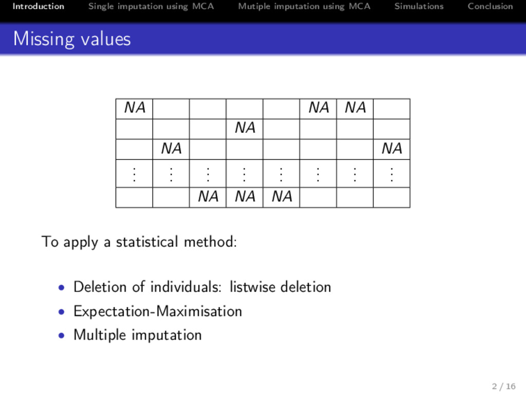
2. Introduction Single imputation using MCA Mutiple imputation using MCA Simulations Conclusion
   Missing values
   NA NA NA
   NA
   NA NA
   .
   .
   .
   .
   .
   .
   .
   .
   .
   .
   .
   .
   .
   .
   .
   .
   .
   .
   .
   .
   .
   .
   .
   .
   NA NA NA
   To apply a statistical method:
   • Deletion of individuals: listwise deletion
   • Expectation-Maximisation
   • Multiple imputation
   2 / 16
   

   View Slide

3. Introduction Single imputation using MCA Mutiple imputation using MCA Simulations Conclusion
   Single imputation
   Notations
   1 0 . . . 1 0 0
   1 0 . . . 1 0 0
   1 0 . . . 1 0 0
   0 1 . . . 0 1 0
   X =
   0 1 . . . 0 0 1
   0 1 . . . 0 1 0
   I1
   0
   DΣ
   =
   ...
   0 IJ
   SVD X, 1
   K
   (DΣ)−1 , 1
   I
   1I −→ XI×J = UI×JΛ1/2
   J×J
   VJ×J
   • principal components: ˆ
   UI×S
   ˆ
   Λ1/2
   S×S
   loadings: ˆ
   VJ×S
   • fitted matrix: ˆ
   XI×J = ˆ
   UI×S
   ˆ
   Λ1/2
   S×S
   ˆ
   VJ×S
   3 / 16
   

   View Slide

4. Introduction Single imputation using MCA Mutiple imputation using MCA Simulations Conclusion
   Iterative MCA (Josse et al., 2012)
   Iterative MCA algorithm:
   4 / 16
   

   View Slide

5. Introduction Single imputation using MCA Mutiple imputation using MCA Simulations Conclusion
   Iterative MCA (Josse et al., 2012)
   Iterative MCA algorithm:
   1 initialization: imputation of the indicator matrix (proportion)
   4 / 16
   

   View Slide

6. Introduction Single imputation using MCA Mutiple imputation using MCA Simulations Conclusion
   Iterative MCA (Josse et al., 2012)
   Iterative MCA algorithm:
   1 initialization: imputation of the indicator matrix (proportion)
   2 iterate until convergence
   (a) perform the MCA, i.e. SVD of X, 1
   K
   (DΣ
   )−1 , 1
   I
   1I
   ˆ
   UI×S , ˆ
   Λ1/2
   S×S
   , ˆ
   VJ×S
   ,
   4 / 16
   

   View Slide

7. Introduction Single imputation using MCA Mutiple imputation using MCA Simulations Conclusion
   Iterative MCA (Josse et al., 2012)
   Iterative MCA algorithm:
   1 initialization: imputation of the indicator matrix (proportion)
   2 iterate until convergence
   (a) perform the MCA, i.e. SVD of X, 1
   K
   (DΣ
   )−1 , 1
   I
   1I
   ˆ
   UI×S , ˆ
   Λ1/2
   S×S
   , ˆ
   VJ×S
   ,
   (b) imputation of the missing values with ˆ
   XI×J
   = ˆ
   UI×S
   ˆ
   Λ1/2
   S×S
   ˆ
   VJ×S
   4 / 16
   

   View Slide

8. Introduction Single imputation using MCA Mutiple imputation using MCA Simulations Conclusion
   Iterative MCA (Josse et al., 2012)
   Iterative MCA algorithm:
   1 initialization: imputation of the indicator matrix (proportion)
   2 iterate until convergence
   (a) perform the MCA, i.e. SVD of X, 1
   K
   (DΣ
   )−1 , 1
   I
   1I
   ˆ
   UI×S , ˆ
   Λ1/2
   S×S
   , ˆ
   VJ×S
   ,
   (b) imputation of the missing values with ˆ
   XI×J
   = ˆ
   UI×S
   ˆ
   Λ1/2
   S×S
   ˆ
   VJ×S
   (c) column margins DΣ
   are updated
   4 / 16
   

   View Slide

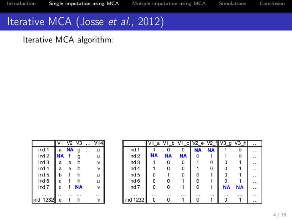
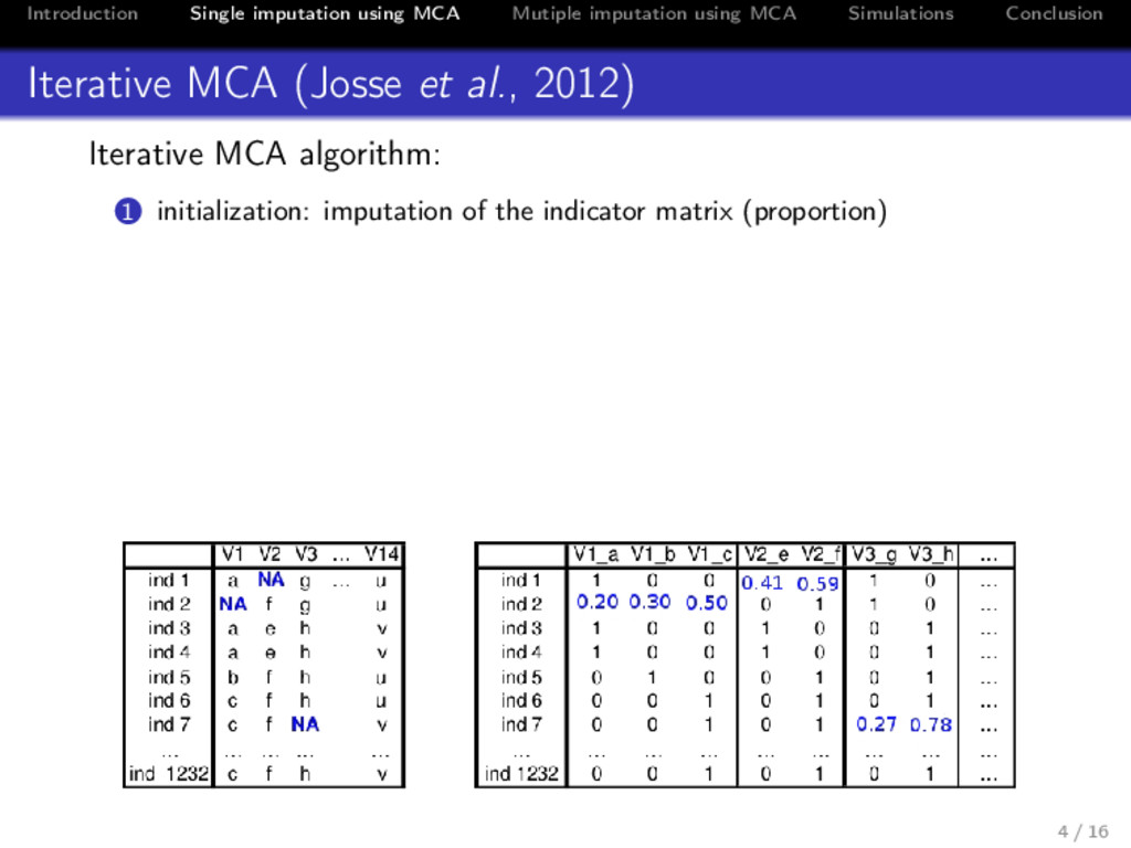
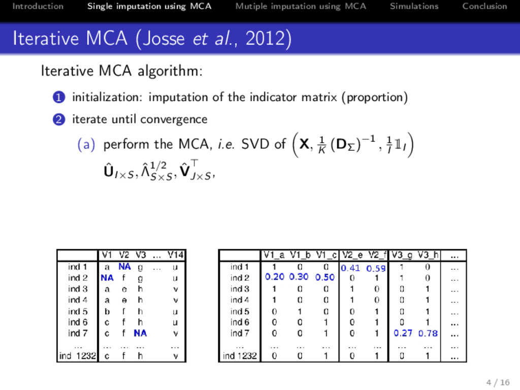
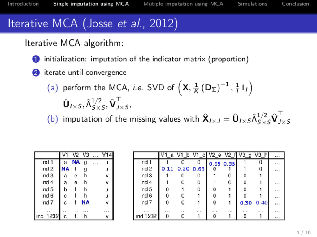
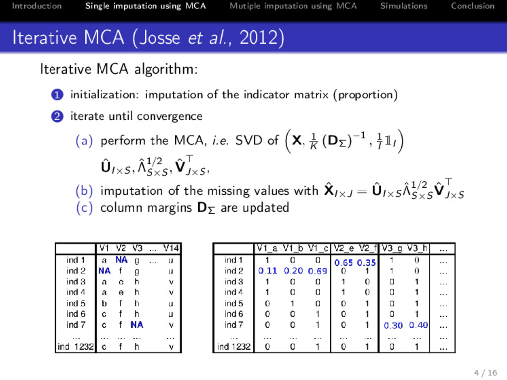
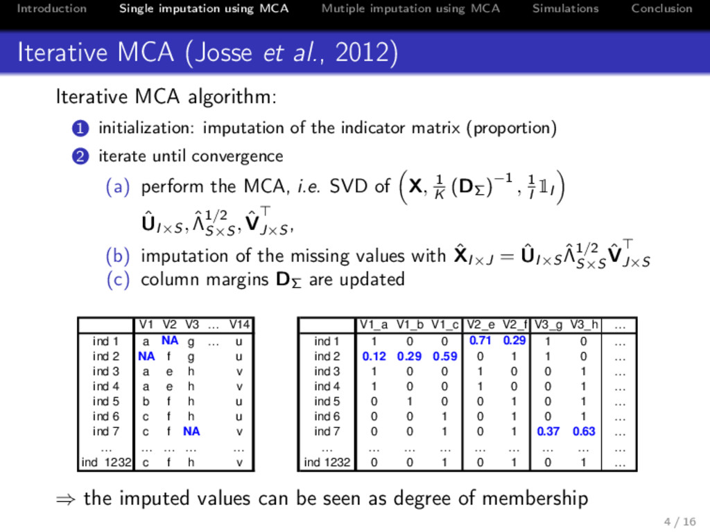
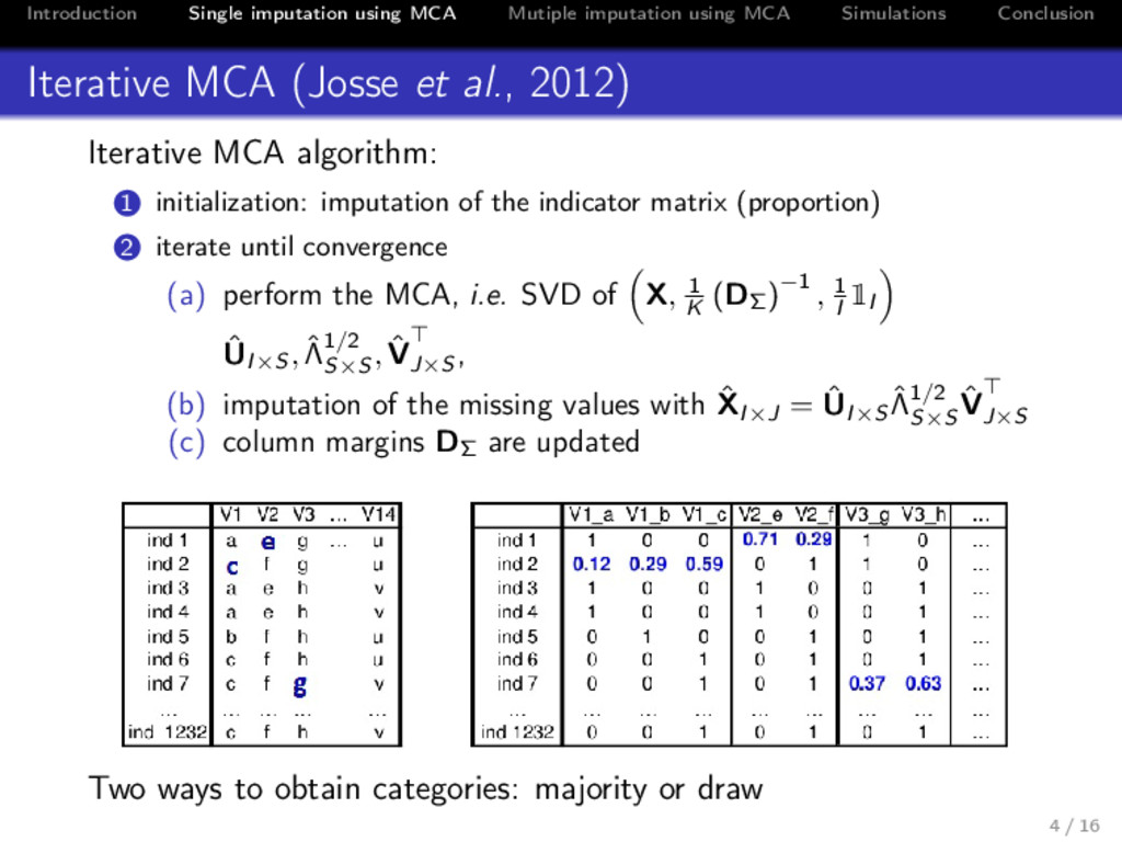
9. Introduction Single imputation using MCA Mutiple imputation using MCA Simulations Conclusion
   Iterative MCA (Josse et al., 2012)
   Iterative MCA algorithm:
   1 initialization: imputation of the indicator matrix (proportion)
   2 iterate until convergence
   (a) perform the MCA, i.e. SVD of X, 1
   K
   (DΣ
   )−1 , 1
   I
   1I
   ˆ
   UI×S , ˆ
   Λ1/2
   S×S
   , ˆ
   VJ×S
   ,
   (b) imputation of the missing values with ˆ
   XI×J
   = ˆ
   UI×S
   ˆ
   Λ1/2
   S×S
   ˆ
   VJ×S
   (c) column margins DΣ
   are updated
   V1 V2 V3 … V14 V1_a V1_b V1_c V2_e V2_f V3_g V3_h …
   ind 1 a NA g … u ind 1 1 0 0 0.71 0.29 1 0 …
   ind 2 NA f g u ind 2 0.12 0.29 0.59 0 1 1 0 …
   ind 3 a e h v ind 3 1 0 0 1 0 0 1 …
   ind 4 a e h v ind 4 1 0 0 1 0 0 1 …
   ind 5 b f h u ind 5 0 1 0 0 1 0 1 …
   ind 6 c f h u ind 6 0 0 1 0 1 0 1 …
   ind 7 c f NA v ind 7 0 0 1 0 1 0.37 0.63 …
   … … … … … … … … … … … … … …
   ind 1232 c f h v ind 1232 0 0 1 0 1 0 1 …
   ⇒ the imputed values can be seen as degree of membership
   4 / 16
   

   View Slide

10. Introduction Single imputation using MCA Mutiple imputation using MCA Simulations Conclusion
    Iterative MCA (Josse et al., 2012)
    Iterative MCA algorithm:
    1 initialization: imputation of the indicator matrix (proportion)
    2 iterate until convergence
    (a) perform the MCA, i.e. SVD of X, 1
    K
    (DΣ
    )−1 , 1
    I
    1I
    ˆ
    UI×S , ˆ
    Λ1/2
    S×S
    , ˆ
    VJ×S
    ,
    (b) imputation of the missing values with ˆ
    XI×J
    = ˆ
    UI×S
    ˆ
    Λ1/2
    S×S
    ˆ
    VJ×S
    (c) column margins DΣ
    are updated
    Two ways to obtain categories: majority or draw
    4 / 16
    

    View Slide

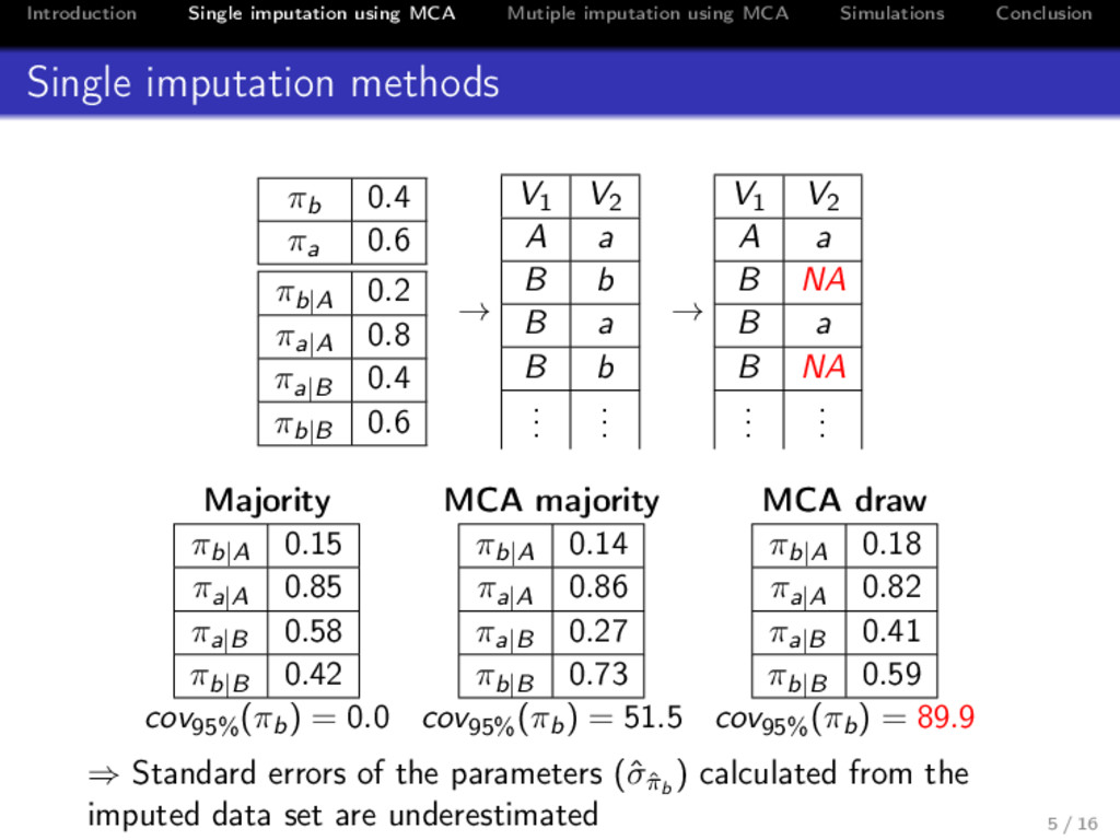
11. Introduction Single imputation using MCA Mutiple imputation using MCA Simulations Conclusion
    Single imputation methods
    πb 0.4
    πa 0.6
    πb|A
    0.2
    πa|A
    0.8
    πa|B
    0.4
    πb|B
    0.6
    →
    V1 V2
    A a
    B b
    B a
    B b
    .
    .
    .
    .
    .
    .
    →
    V1 V2
    A a
    B NA
    B a
    B NA
    .
    .
    .
    .
    .
    .
    Majority MCA majority MCA draw
    πb|A
    0.15
    πa|A
    0.85
    πa|B
    0.58
    πb|B
    0.42
    πb|A
    0.14
    πa|A
    0.86
    πa|B
    0.27
    πb|B
    0.73
    πb|A
    0.18
    πa|A
    0.82
    πa|B
    0.41
    πb|B
    0.59
    cov95%
    (πb) = 0.0 cov95%
    (πb) = 51.5 cov95%
    (πb) = 89.9
    ⇒ Standard errors of the parameters (ˆ
    σˆ
    πb
    ) calculated from the
    imputed data set are underestimated 5 / 16
    

    View Slide

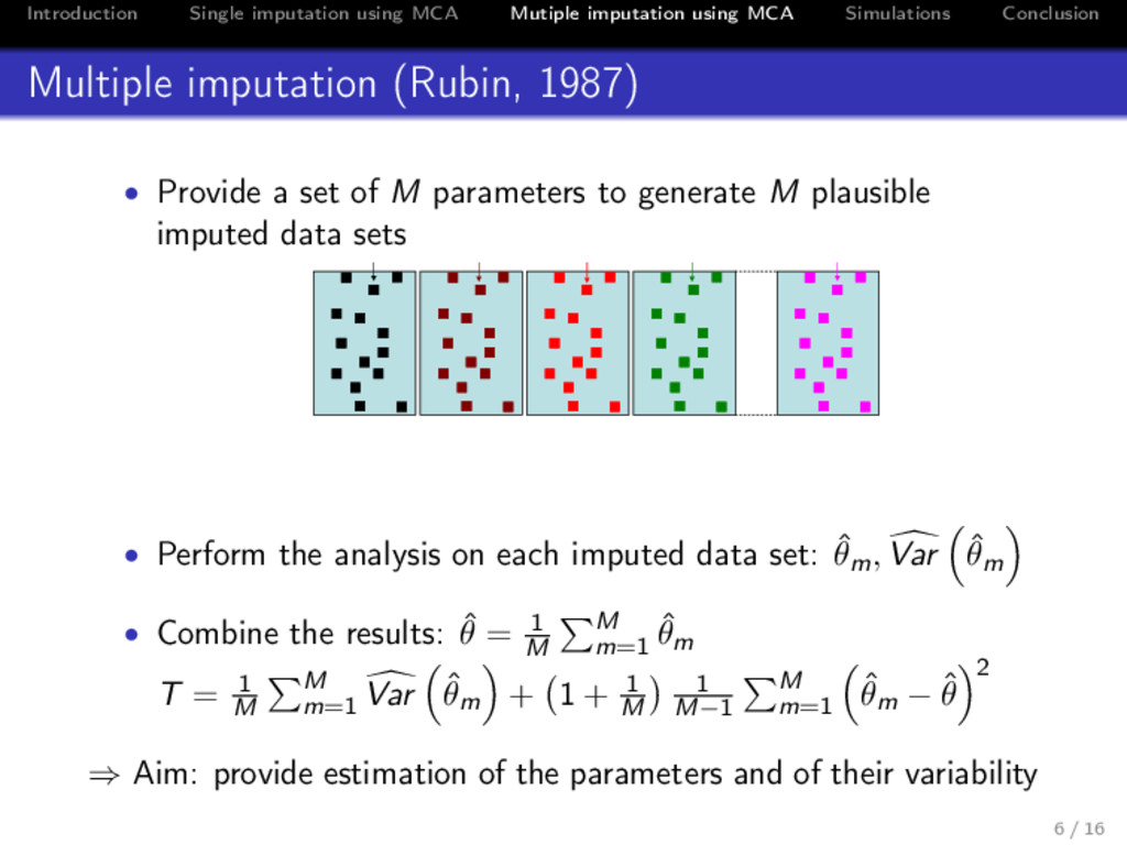
12. Introduction Single imputation using MCA Mutiple imputation using MCA Simulations Conclusion
    Multiple imputation (Rubin, 1987)
    • Provide a set of M parameters to generate M plausible
    imputed data sets
    ( ˆ
    F ˆ
    u′)ij
    ( ˆ
    F ˆ
    u′)1
    ij
    + ε1
    ij
    ( ˆ
    F ˆ
    u′)2
    ij
    + ε2
    ij
    ( ˆ
    F ˆ
    u′)3
    ij
    + ε3
    ij
    ( ˆ
    F ˆ
    u′)B
    ij
    + εB
    ij
    • Perform the analysis on each imputed data set: ˆ
    θm, Var ˆ
    θm
    • Combine the results: ˆ
    θ = 1
    M
    M
    m=1
    ˆ
    θm
    T = 1
    M
    M
    m=1
    Var ˆ
    θm + 1 + 1
    M
    1
    M−1
    M
    m=1
    ˆ
    θm − ˆ
    θ
    2
    ⇒ Aim: provide estimation of the parameters and of their variability
    6 / 16
    

    View Slide

13. Introduction Single imputation using MCA Mutiple imputation using MCA Simulations Conclusion
    Multiple imputation (Rubin, 1987)
    • Provide a set of M parameters to generate M plausible
    imputed data sets
    ( ˆ
    F ˆ
    u′)ij
    ( ˆ
    F ˆ
    u′)1
    ij
    + ε1
    ij
    ( ˆ
    F ˆ
    u′)2
    ij
    + ε2
    ij
    ( ˆ
    F ˆ
    u′)3
    ij
    + ε3
    ij
    ( ˆ
    F ˆ
    u′)B
    ij
    + εB
    ij
    Bayesian or Bootstrap approach
    • Perform the analysis on each imputed data set: ˆ
    θm, Var ˆ
    θm
    • Combine the results: ˆ
    θ = 1
    M
    M
    m=1
    ˆ
    θm
    T = 1
    M
    M
    m=1
    Var ˆ
    θm + 1 + 1
    M
    1
    M−1
    M
    m=1
    ˆ
    θm − ˆ
    θ
    2
    ⇒ Aim: provide estimation of the parameters and of their variability
    6 / 16
    

    View Slide

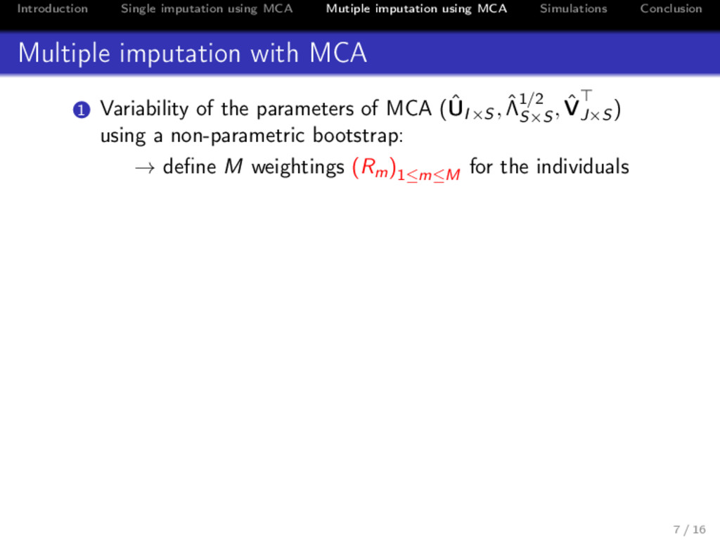
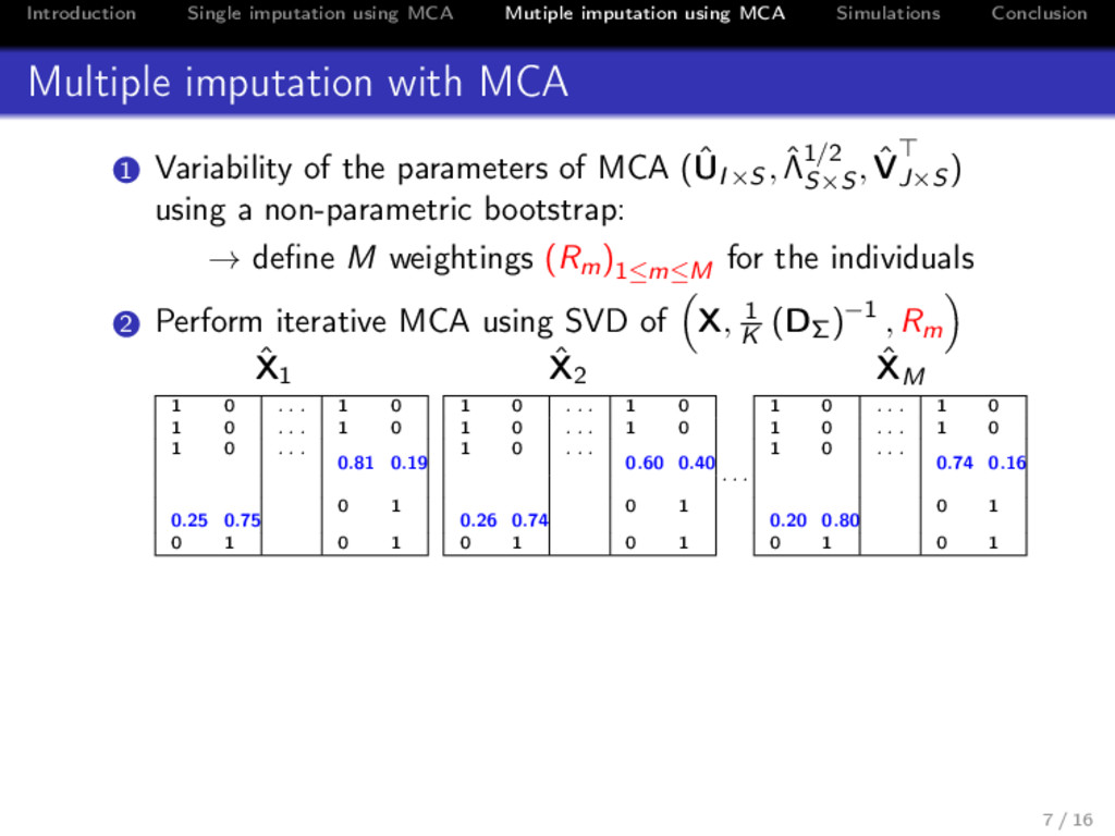
14. Introduction Single imputation using MCA Mutiple imputation using MCA Simulations Conclusion
    Multiple imputation with MCA
    1 Variability of the parameters of MCA (ˆ
    UI×S , ˆ
    Λ1/2
    S×S
    , ˆ
    VJ×S
    )
    using a non-parametric bootstrap:
    → define M weightings (Rm)1≤m≤M
    for the individuals
    7 / 16
    

    View Slide

15. Introduction Single imputation using MCA Mutiple imputation using MCA Simulations Conclusion
    Multiple imputation with MCA
    1 Variability of the parameters of MCA (ˆ
    UI×S , ˆ
    Λ1/2
    S×S
    , ˆ
    VJ×S
    )
    using a non-parametric bootstrap:
    → define M weightings (Rm)1≤m≤M
    for the individuals
    2 Perform iterative MCA using SVD of X, 1
    K
    (DΣ)−1 , Rm
    ˆ
    X1
    ˆ
    X2
    ˆ
    XM
    1 0 . . . 1 0
    1 0 . . . 1 0
    1 0 . . .
    0.81 0.19
    0.25 0.75
    0 1
    0 1 0 1
    1 0 . . . 1 0
    1 0 . . . 1 0
    1 0 . . .
    0.60 0.40
    0.26 0.74
    0 1
    0 1 0 1
    . . .
    1 0 . . . 1 0
    1 0 . . . 1 0
    1 0 . . .
    0.74 0.16
    0.20 0.80
    0 1
    0 1 0 1
    7 / 16
    

    View Slide

16. Introduction Single imputation using MCA Mutiple imputation using MCA Simulations Conclusion
    Multiple imputation with MCA
    1 Variability of the parameters of MCA (ˆ
    UI×S , ˆ
    Λ1/2
    S×S
    , ˆ
    VJ×S
    )
    using a non-parametric bootstrap:
    → define M weightings (Rm)1≤m≤M
    for the individuals
    2 Perform iterative MCA using SVD of X, 1
    K
    (DΣ)−1 , Rm
    ˆ
    X1
    ˆ
    X2
    ˆ
    XM
    1 0 . . . 1 0
    1 0 . . . 1 0
    1 0 . . .
    0.81 0.19
    0.25 0.75
    0 1
    0 1 0 1
    1 0 . . . 1 0
    1 0 . . . 1 0
    1 0 . . .
    0.60 0.40
    0.26 0.74
    0 1
    0 1 0 1
    . . .
    1 0 . . . 1 0
    1 0 . . . 1 0
    1 0 . . .
    0.74 0.16
    0.20 0.80
    0 1
    0 1 0 1
    3 Draw categories from the values of ˆ
    Xm
    1≤m≤M
    A . . . A
    A . . . A
    A . . .
    B
    B
    . . . C
    B . . . B
    A . . . A
    A . . . A
    A . . .
    A
    B
    . . . C
    B . . . B
    . . .
    A . . . A
    A . . . A
    A . . .
    B
    B
    . . . C
    B . . . B
    7 / 16
    

    View Slide

17. Introduction Single imputation using MCA Mutiple imputation using MCA Simulations Conclusion
    Properties
    Multiple imputation using MCA:
    • captures the relationships between variables
    • captures the similarities between individuals
    • requires a small number of parameters
    • can be applied on various data sets:
    • small or large number of variables/categories
    • small or large number of individuals
    8 / 16
    

    View Slide

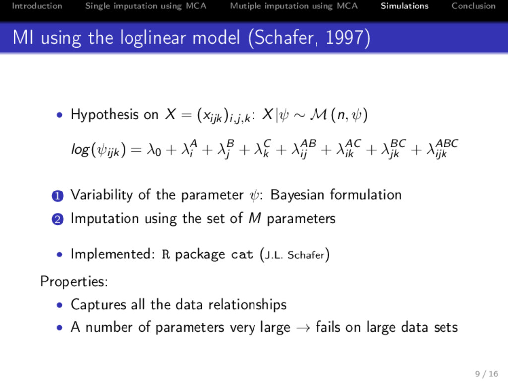
18. Introduction Single imputation using MCA Mutiple imputation using MCA Simulations Conclusion
    MI using the loglinear model (Schafer, 1997)
    • Hypothesis on X = (xijk)i,j,k: X|ψ ∼ M (n, ψ)
    log(ψijk) = λ0 + λA
    i
    + λB
    j
    + λC
    k
    + λAB
    ij
    + λAC
    ik
    + λBC
    jk
    + λABC
    ijk
    1 Variability of the parameter ψ: Bayesian formulation
    2 Imputation using the set of M parameters
    • Implemented: R package cat (J.L. Schafer)
    Properties:
    • Captures all the data relationships
    • A number of parameters very large → fails on large data sets
    9 / 16
    

    View Slide

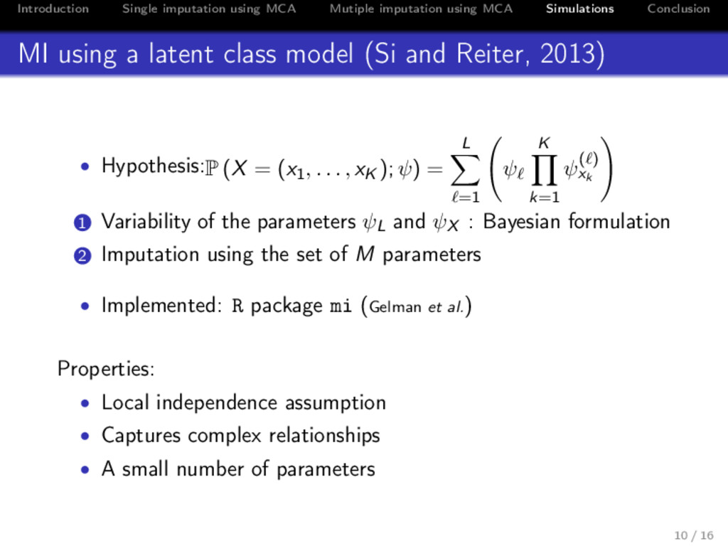
19. Introduction Single imputation using MCA Mutiple imputation using MCA Simulations Conclusion
    MI using a latent class model (Si and Reiter, 2013)
    • Hypothesis:P (X = (x1, . . . , xK ); ψ) =
    L
    =1
    ψ
    K
    k=1
    ψ( )
    xk
    1 Variability of the parameters ψL and ψX : Bayesian formulation
    2 Imputation using the set of M parameters
    • Implemented: R package mi (Gelman et al.)
    Properties:
    • Local independence assumption
    • Captures complex relationships
    • A small number of parameters
    10 / 16
    

    View Slide

20. Introduction Single imputation using MCA Mutiple imputation using MCA Simulations Conclusion
    Conditional modelling (van Buuren, 2006)
    General principle:
    • specify one conditional model per incomplete variable
    • incomplete variables are successively imputed
    • cycle through variables
    • repeat M times
    Implemented: R package MICE (Stef van Buuren)
    Properties:
    • More flexible
    • Time consuming
    11 / 16
    

    View Slide

21. Introduction Single imputation using MCA Mutiple imputation using MCA Simulations Conclusion
    Conditional modelling
    • A standard one: one logistic regression model/variable
    without interaction
    Properties: captures relationships between pairs of variables
    • A recent one: one random forest/variable (Doove et al.,
    2014)
    Properties:
    • non-parametric modelling
    • captures complex relationships between variables
    12 / 16
    

    View Slide

22. Introduction Single imputation using MCA Mutiple imputation using MCA Simulations Conclusion
    Simulations from real data sets
    • Quantities of interest: θ = parameters of a logistic model
    • 200 simulations from real data sets
    • the real data set is considered as a population
    • drawn one sample from the data set
    • generate 20% of missing values
    • multiple imputation using M = 5 imputed arrays
    • Criteria
    • bias
    • CI width, coverage
    13 / 16
    

    View Slide

23. Introduction Single imputation using MCA Mutiple imputation using MCA Simulations Conclusion
    Results - Inference
    q
    MIMCA 5
    Loglinear
    Latent class
    FCS−log
    FCS−rf
    0.80
    0.85
    0.90
    0.95
    1.00
    Titanic
    coverage
    q
    q
    q
    q
    MIMCA 2
    Loglinear
    Latent class
    FCS−log
    FCS−rf
    0.80
    0.85
    0.90
    0.95
    1.00
    Galetas
    coverage
    q
    MIMCA 5
    Latent class
    FCS−log
    FCS−rf
    0.80
    0.85
    0.90
    0.95
    1.00
    Income
    coverage
    Titanic Galetas Income
    Number of variables 4 4 14
    Number of categories ≤ 4 ≤ 11 ≤ 9
    14 / 16
    

    View Slide

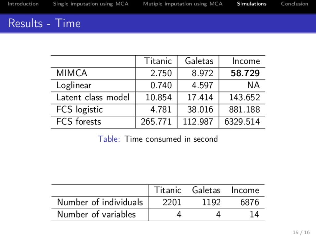
24. Introduction Single imputation using MCA Mutiple imputation using MCA Simulations Conclusion
    Results - Time
    Titanic Galetas Income
    MIMCA 2.750 8.972 58.729
    Loglinear 0.740 4.597 NA
    Latent class model 10.854 17.414 143.652
    FCS logistic 4.781 38.016 881.188
    FCS forests 265.771 112.987 6329.514
    Table: Time consumed in second
    Titanic Galetas Income
    Number of individuals 2201 1192 6876
    Number of variables 4 4 14
    15 / 16
    

    View Slide

25. Introduction Single imputation using MCA Mutiple imputation using MCA Simulations Conclusion
    Conclusion
    A new multiple imputation method based on MCA
    Strongest point: dimensionality reduction method
    • captures the relationships between variables
    • captures the similarities between individuals
    • requires a small number of parameters
    From a practical point of view:
    • can be applied on data sets of various dimensions
    (many categories or not / few individuals or not)
    • provides correct inferences and performs quickly
    • a tuning parameter: the number of dimensions
    Perspective:
    • mixed data
    16 / 16
    

    View Slide