Random Forests versus PCA

Transcript

1. Random Forest Principal component Results Imputation for mixed data: Random Forest versus PCA Vincent Audigier, François Husson & Julie Josse Agrocampus Rennes ERCIM 2013, London, 14-12-2013 1 / 20
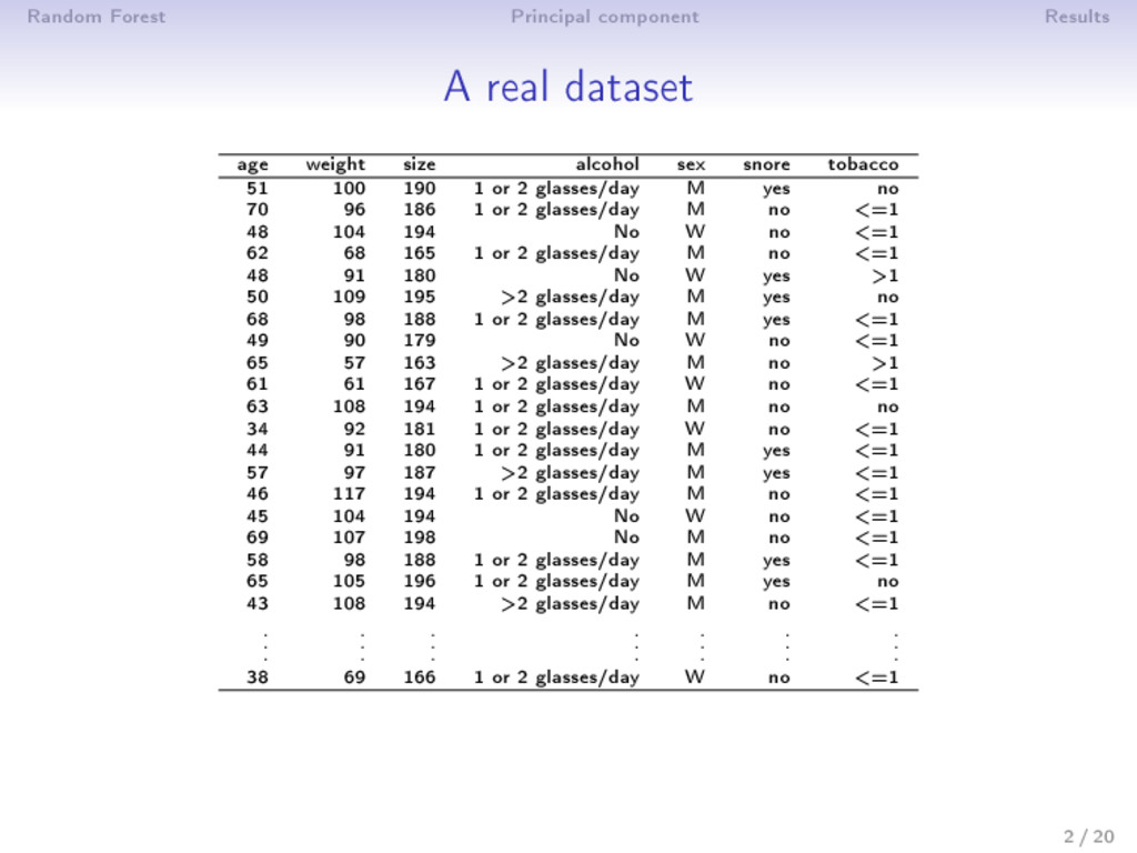
2. Random Forest Principal component Results A real dataset age weight size alcohol sex snore tobacco 51 100 190 1 or 2 glasses/day M yes no 70 96 186 1 or 2 glasses/day M no <=1 48 104 194 No W no <=1 62 68 165 1 or 2 glasses/day M no <=1 48 91 180 No W yes >1 50 109 195 >2 glasses/day M yes no 68 98 188 1 or 2 glasses/day M yes <=1 49 90 179 No W no <=1 65 57 163 >2 glasses/day M no >1 61 61 167 1 or 2 glasses/day W no <=1 63 108 194 1 or 2 glasses/day M no no 34 92 181 1 or 2 glasses/day W no <=1 44 91 180 1 or 2 glasses/day M yes <=1 57 97 187 >2 glasses/day M yes <=1 46 117 194 1 or 2 glasses/day M no <=1 45 104 194 No W no <=1 69 107 198 No M no <=1 58 98 188 1 or 2 glasses/day M yes <=1 65 105 196 1 or 2 glasses/day M yes no 43 108 194 >2 glasses/day M no <=1 . . . . . . . . . . . . . . . . . . . . . 38 69 166 1 or 2 glasses/day W no <=1 2 / 20
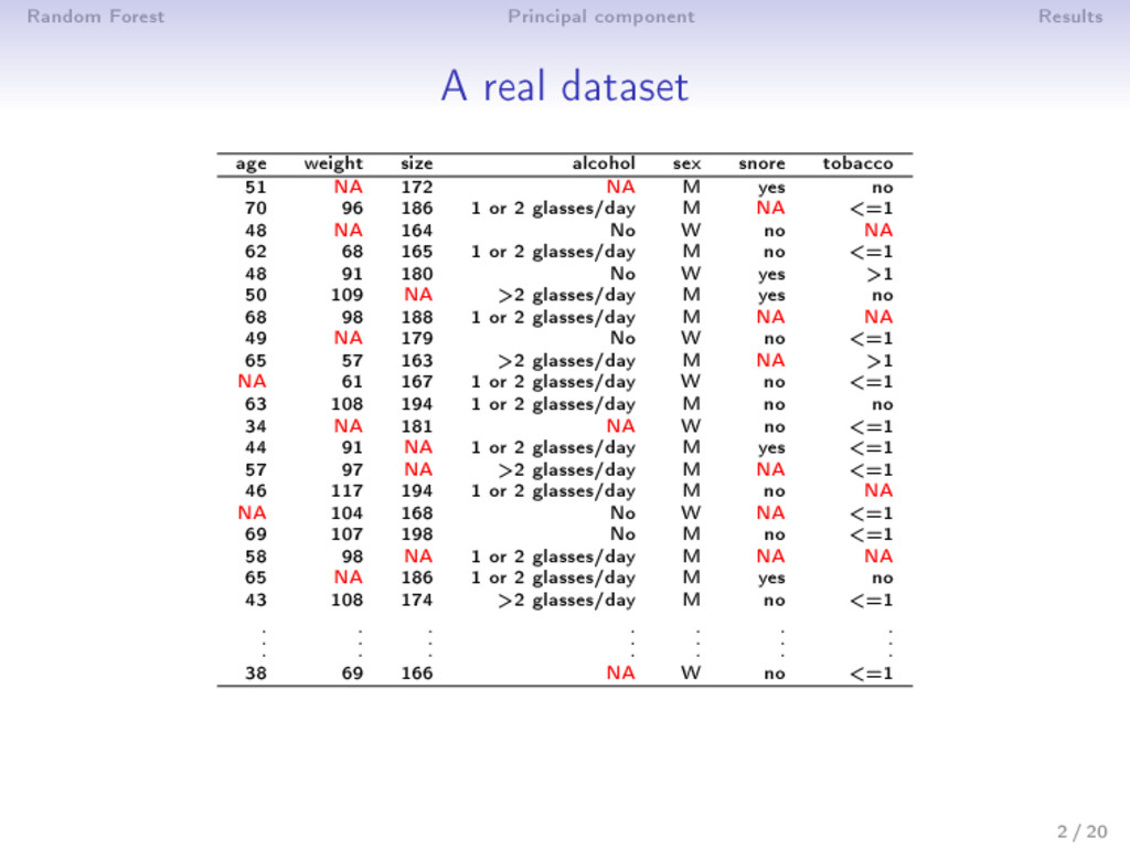
3. Random Forest Principal component Results A real dataset age weight size alcohol sex snore tobacco 51 NA 172 NA M yes no 70 96 186 1 or 2 glasses/day M NA <=1 48 NA 164 No W no NA 62 68 165 1 or 2 glasses/day M no <=1 48 91 180 No W yes >1 50 109 NA >2 glasses/day M yes no 68 98 188 1 or 2 glasses/day M NA NA 49 NA 179 No W no <=1 65 57 163 >2 glasses/day M NA >1 NA 61 167 1 or 2 glasses/day W no <=1 63 108 194 1 or 2 glasses/day M no no 34 NA 181 NA W no <=1 44 91 NA 1 or 2 glasses/day M yes <=1 57 97 NA >2 glasses/day M NA <=1 46 117 194 1 or 2 glasses/day M no NA NA 104 168 No W NA <=1 69 107 198 No M no <=1 58 98 NA 1 or 2 glasses/day M NA NA 65 NA 186 1 or 2 glasses/day M yes no 43 108 174 >2 glasses/day M no <=1 . . . . . . . . . . . . . . . . . . . . . 38 69 166 NA W no <=1 2 / 20
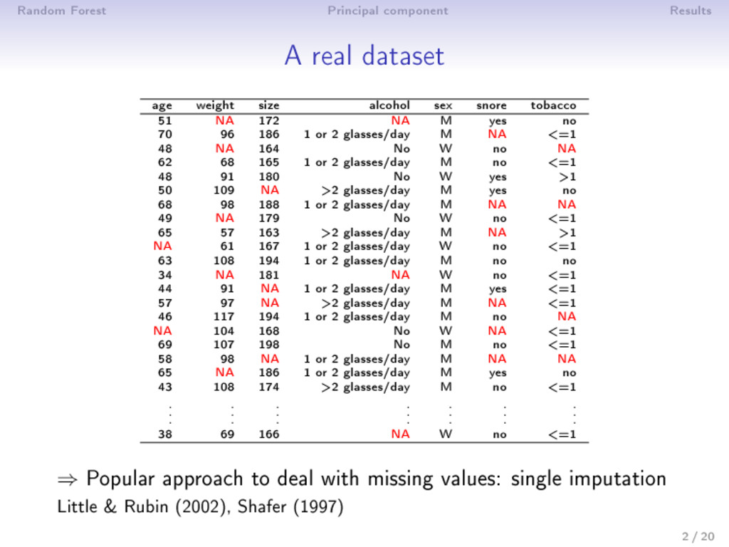
4. Random Forest Principal component Results A real dataset age weight size alcohol sex snore tobacco 51 NA 172 NA M yes no 70 96 186 1 or 2 glasses/day M NA <=1 48 NA 164 No W no NA 62 68 165 1 or 2 glasses/day M no <=1 48 91 180 No W yes >1 50 109 NA >2 glasses/day M yes no 68 98 188 1 or 2 glasses/day M NA NA 49 NA 179 No W no <=1 65 57 163 >2 glasses/day M NA >1 NA 61 167 1 or 2 glasses/day W no <=1 63 108 194 1 or 2 glasses/day M no no 34 NA 181 NA W no <=1 44 91 NA 1 or 2 glasses/day M yes <=1 57 97 NA >2 glasses/day M NA <=1 46 117 194 1 or 2 glasses/day M no NA NA 104 168 No W NA <=1 69 107 198 No M no <=1 58 98 NA 1 or 2 glasses/day M NA NA 65 NA 186 1 or 2 glasses/day M yes no 43 108 174 >2 glasses/day M no <=1 . . . . . . . . . . . . . . . . . . . . . 38 69 166 NA W no <=1 ⇒ Popular approach to deal with missing values: single imputation Little & Rubin (2002), Shafer (1997) 2 / 20
5. Random Forest Principal component Results Single imputation methods Continuous variables: k-nearest neighbors, joint modeling: normal distribution, conditional modeling (van Bureen 1999): iterative regressions, etc. Categorical variables: k-nn, joint modeling: log-linear model, latent class model (Vermunt, 2008), conditional modeling: iterative logistic regressions, etc. Mixed data: • General location model (Schaefer, 1997) • Transform the categorical variables into dummy variables and deal as continuous variables (package Amelia) • MICE (conditional multivariate imputation by chained equations, van Bureen 1999): a model must be specied for each variable - iterative linear and logistic regressions (package mice) ⇒ Random forests (Stekhoven & Bühlmann, 2011) ⇒ Principal component method (Audigier, Husson & Josse, 2013) 3 / 20
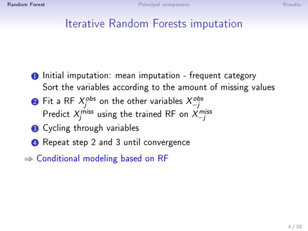
6. Random Forest Principal component Results Iterative Random Forests imputation 1 Initial imputation: mean imputation - frequent category Sort the variables according to the amount of missing values 2 Fit a RF X obs j on the other variables X obs −j Predict X miss j using the trained RF on X miss −j 3 Cycling through variables 4 Repeat step 2 and 3 until convergence ⇒ Conditional modeling based on RF 4 / 20
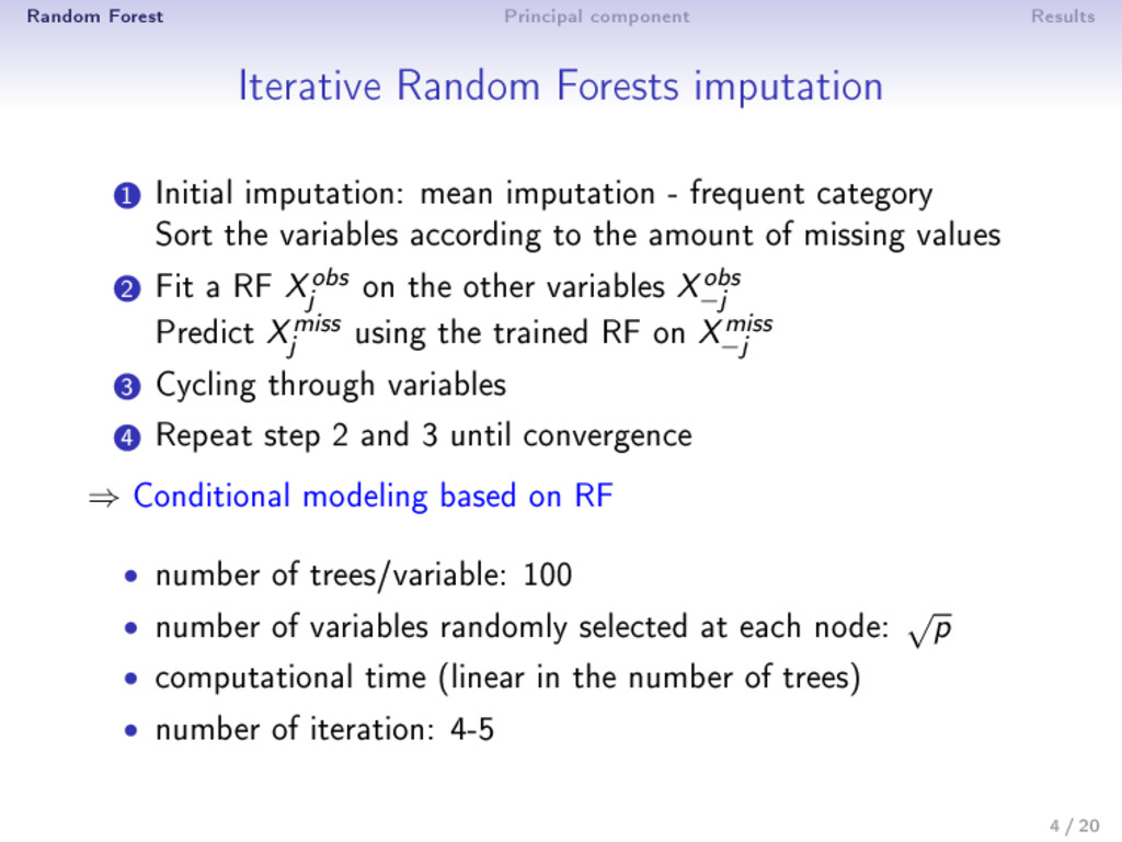
7. Random Forest Principal component Results Iterative Random Forests imputation 1 Initial imputation: mean imputation - frequent category Sort the variables according to the amount of missing values 2 Fit a RF X obs j on the other variables X obs −j Predict X miss j using the trained RF on X miss −j 3 Cycling through variables 4 Repeat step 2 and 3 until convergence ⇒ Conditional modeling based on RF • number of trees/variable: 100 • number of variables randomly selected at each node: √ p • computational time (linear in the number of trees) • number of iteration: 4-5 4 / 20
8. Random Forest Principal component Results Iterative Random Forests imputation ⇒ Properties: • Non-linear relations • Complex interactions • np (dicult with MICE: ridge regression per variable) • OOB: approximation of the imputation error ⇒ Outperforms k-nn and MICE 5 / 20
9. Random Forest Principal component Results PCA with missing values ⇒ PCA: least squares Xn×p − Un×SΛ 1 2 S×SVp×S) 2 • F = UΛ1 2 principal components - scores • V principal axes - loadings ⇒ PCA with missing values: weighted least squares Wn×p ∗ (Xn×p − Un×SΛ 1 2 S×SVp×S) 2 with wij = 0 if xij is missing, wij = 1 otherwise Many algorithms: weighted alternating least squares (Gabriel & Zamir, 1979); iterative PCA (Kiers, 1997) 6 / 20
10. Random Forest Principal component Results Iterative PCA algorithm The data set -2 -1 0 1 2 3 -2 -1 0 1 2 3 x1 x2 x1 x2 -2.0 -2.01 -1.5 -1.48 0.0 -0.01 1.5 NA 2.0 1.98 7 / 20
11. Random Forest Principal component Results Iterative PCA algorithm Initialization step: mean imputation -2 -1 0 1 2 3 -2 -1 0 1 2 3 x1 x2 x1 x2 -2.0 -2.01 -1.5 -1.48 0.0 -0.01 1.5 NA 2.0 1.98 x1 x2 -2.0 -2.01 -1.5 -1.48 0.0 -0.01 1.5 0.00 2.0 1.98 7 / 20
12. Random Forest Principal component Results Iterative PCA algorithm PCA performed on the completed data set; 1 dimension is kept -2 -1 0 1 2 3 -2 -1 0 1 2 3 x1 x2 x1 x2 -2.0 -2.01 -1.5 -1.48 0.0 -0.01 1.5 NA 2.0 1.98 x1 x2 -2.0 -2.01 -1.5 -1.48 0.0 -0.01 1.5 0.00 2.0 1.98 x1 x2 -1.98 -2.04 -1.44 -1.56 0.15 -0.18 1.00 0.57 2.27 1.67 7 / 20
13. Random Forest Principal component Results Iterative PCA algorithm Calculation of the model prediction -2 -1 0 1 2 3 -2 -1 0 1 2 3 x1 x2 x1 x2 -2.0 -2.01 -1.5 -1.48 0.0 -0.01 1.5 NA 2.0 1.98 x1 x2 -2.0 -2.01 -1.5 -1.48 0.0 -0.01 1.5 0.00 2.0 1.98 x1 x2 -1.98 -2.04 -1.44 -1.56 0.15 -0.18 1.00 0.57 2.27 1.67 7 / 20
14. Random Forest Principal component Results Iterative PCA algorithm Imputation step: X = W ∗ X + (1 − W) ∗ ˆ X -2 -1 0 1 2 3 -2 -1 0 1 2 3 x1 x2 x1 x2 -2.0 -2.01 -1.5 -1.48 0.0 -0.01 1.5 NA 2.0 1.98 x1 x2 -2.0 -2.01 -1.5 -1.48 0.0 -0.01 1.5 0.00 2.0 1.98 x1 x2 -1.98 -2.04 -1.44 -1.56 0.15 -0.18 1.00 0.57 2.27 1.67 x1 x2 -2.0 -2.01 -1.5 -1.48 0.0 -0.01 1.5 0.57 2.0 1.98 7 / 20
15. Random Forest Principal component Results Iterative PCA algorithm PCA is performed; 1 dimension is kept x1 x2 -2.0 -2.01 -1.5 -1.48 0.0 -0.01 1.5 NA 2.0 1.98 x1 x2 -2.0 -2.01 -1.5 -1.48 0.0 -0.01 1.5 0.57 2.0 1.98 x1 x2 -2.0 -2.01 -1.5 -1.48 0.0 -0.01 1.5 0.57 2.0 1.98 -2 -1 0 1 2 3 -2 -1 0 1 2 3 x1 x2 7 / 20
16. Random Forest Principal component Results Iterative PCA algorithm Imputation step: X = W ∗ X + (1 − W) ∗ ˆ X x1 x2 -2.0 -2.01 -1.5 -1.48 0.0 -0.01 1.5 NA 2.0 1.98 x1 x2 -2.0 -2.01 -1.5 -1.48 0.0 -0.01 1.5 0.57 2.0 1.98 x1 x2 -2.00 -2.01 -1.47 -1.52 0.09 -0.11 1.20 0.90 2.18 1.78 x1 x2 -2.0 -2.01 -1.5 -1.48 0.0 -0.01 1.5 0.90 2.0 1.98 -2 -1 0 1 2 3 -2 -1 0 1 2 3 x1 x2 7 / 20
17. Random Forest Principal component Results Iterative PCA algorithm Iterate until convergence x1 x2 -2.0 -2.01 -1.5 -1.48 0.0 -0.01 1.5 NA 2.0 1.98 x1 x2 -2.0 -2.01 -1.5 -1.48 0.0 -0.01 1.5 0.00 2.0 1.98 x1 x2 -1.98 -2.04 -1.44 -1.56 0.15 -0.18 1.00 0.57 2.27 1.67 x1 x2 -2.0 -2.01 -1.5 -1.48 0.0 -0.01 1.5 0.57 2.0 1.98 -2 -1 0 1 2 3 -2 -1 0 1 2 3 x1 x2 7 / 20
18. Random Forest Principal component Results Iterative PCA - convergence Imputed values are obtained at convergence x1 x2 -2.0 -2.01 -1.5 -1.48 0.0 -0.01 1.5 NA 2.0 1.98 x1 x2 -2.0 -2.01 -1.5 -1.48 0.0 -0.01 1.5 1.46 2.0 1.98 -2 -1 0 1 2 3 -2 -1 0 1 2 3 x1 x2 8 / 20
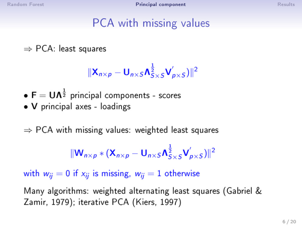
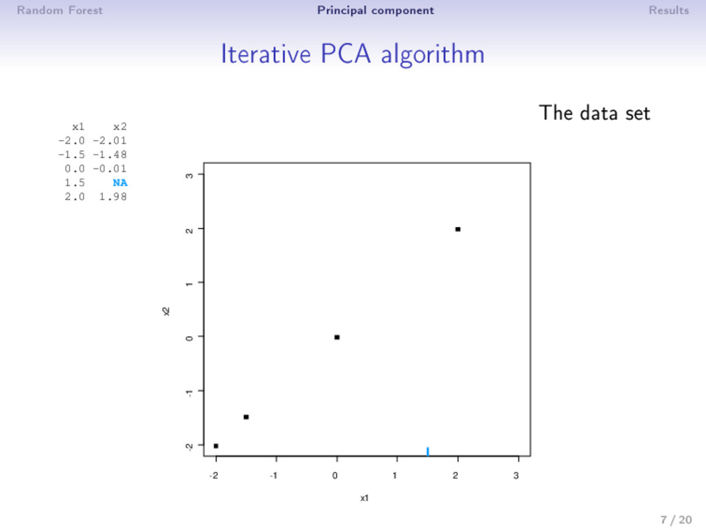
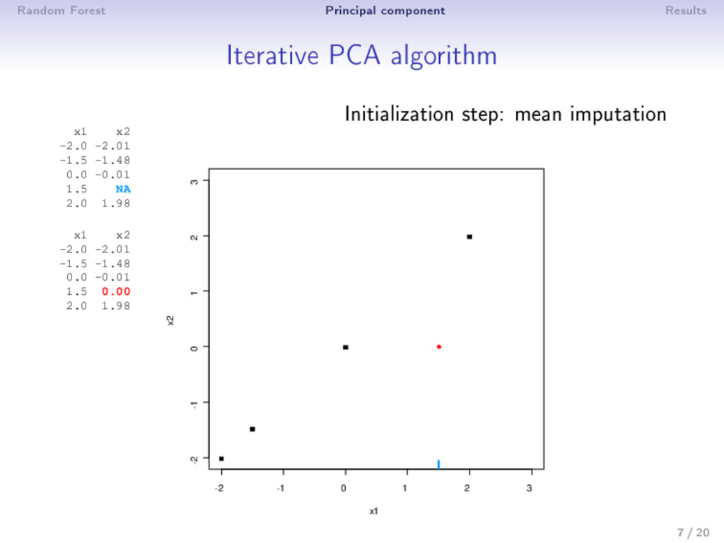
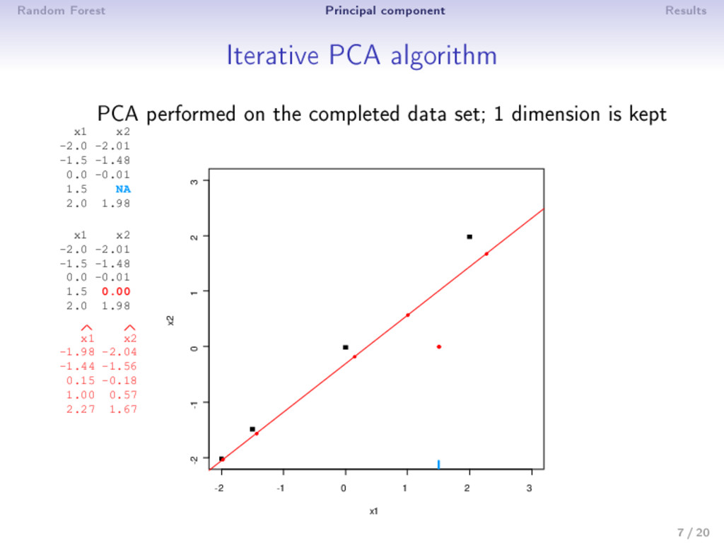
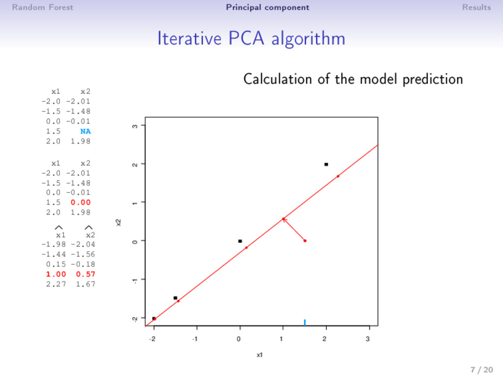
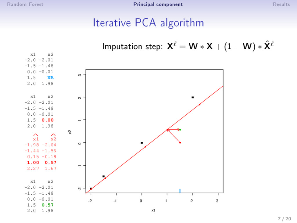
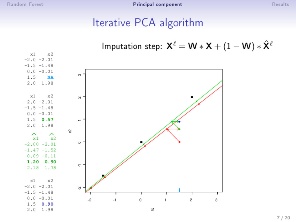
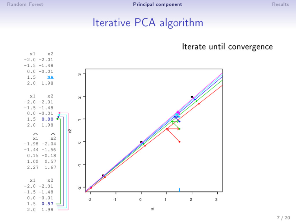
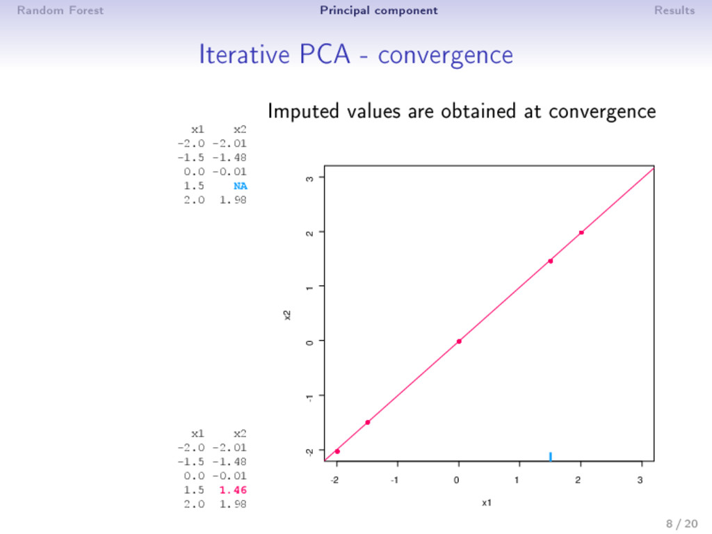
19. Random Forest Principal component Results Iterative PCA 1 initialization = 0: X0 (mean imputation) 2 step : (a) PCA on the completed matrix X −1 → (U , Λ , V ) S dimensions are kept; ˆ X = U Λ1/2 V (estimation) (b) X = W ∗ X+ (1 − W) ∗ ˆ X (imputation) 3 Estimation and imputation are repeated until convergence • The number of dimensions S has to be chosen a priori • An imputation is performed during the algorithm ⇒ PCA can be seen as an imputation method • Overtting problems are dealt with a regularized algorithm 9 / 20
20. Random Forest Principal component Results Principal component method for mixed data (complete case) Factorial Analysis on Mixed Data (Escoer, 1979), PCAMIX (Kiers, 1991) Categorical variables Continuous variables 0 1 0 1 0 centring & scaling I1 I2 Ik division by and centring I/Ik 0 1 0 1 0 0 1 0 0 1 51 100 190 70 96 196 38 69 166 0 1 1 0 1 0 1 0 0 0 1 0 0 1 0 Indicator matrix Matrix which balances the influence of each variable A PCA is performed on the weighted matrix 10 / 20
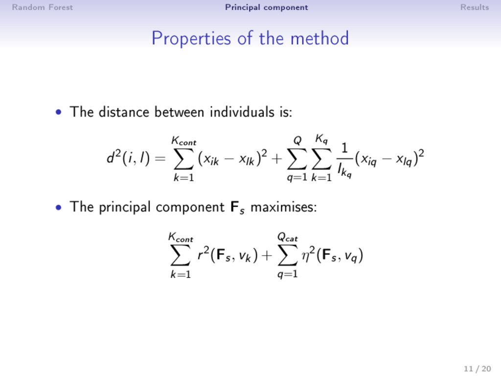
21. Random Forest Principal component Results Properties of the method • The distance between individuals is: d 2(i , l ) = Kcont k=1 (xik − xlk)2 + Q q=1 Kq k=1 1 Ikq (xiq − xlq)2 • The principal component Fs maximises: Kcont k=1 r 2(Fs, vk) + Qcat q=1 η2(Fs, vq) 11 / 20
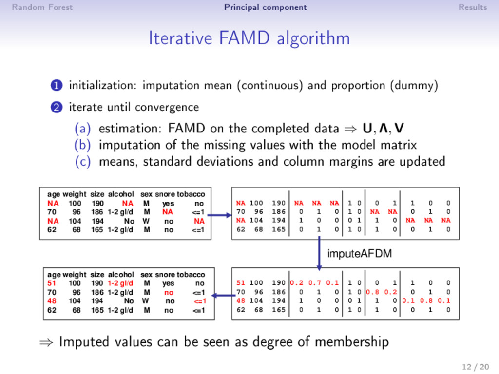
22. Random Forest Principal component Results Iterative FAMD algorithm 1 initialization: imputation mean (continuous) and proportion (dummy) 2 iterate until convergence (a) estimation: FAMD on the completed data ⇒ U, Λ, V (b) imputation of the missing values with the model matrix (c) means, standard deviations and column margins are updated age weight size alcohol sex snore tobacco NA 100 190 NA M yes no 70 96 186 1-2 gl/d M NA <=1 NA 104 194 No W no NA 62 68 165 1-2 gl/d M no <=1 age weight size alcohol sex snore tobacco 51 100 190 1-2 gl/d M yes no 70 96 186 1-2 gl/d M no <=1 48 104 194 No W no <=1 62 68 165 1-2 gl/d M no <=1 51 100 190 0.2 0.7 0.1 1 0 0 1 1 0 0 70 96 186 0 1 0 1 0 0.8 0.2 0 1 0 48 104 194 1 0 0 0 1 1 0 0.1 0.8 0.1 62 68 165 0 1 0 1 0 1 0 0 1 0 NA 100 190 NA NA NA 1 0 0 1 1 0 0 70 96 186 0 1 0 1 0 NA NA 0 1 0 NA 104 194 1 0 0 0 1 1 0 NA NA NA 62 68 165 0 1 0 1 0 1 0 0 1 0 imputeAFDM ⇒ Imputed values can be seen as degree of membership 12 / 20
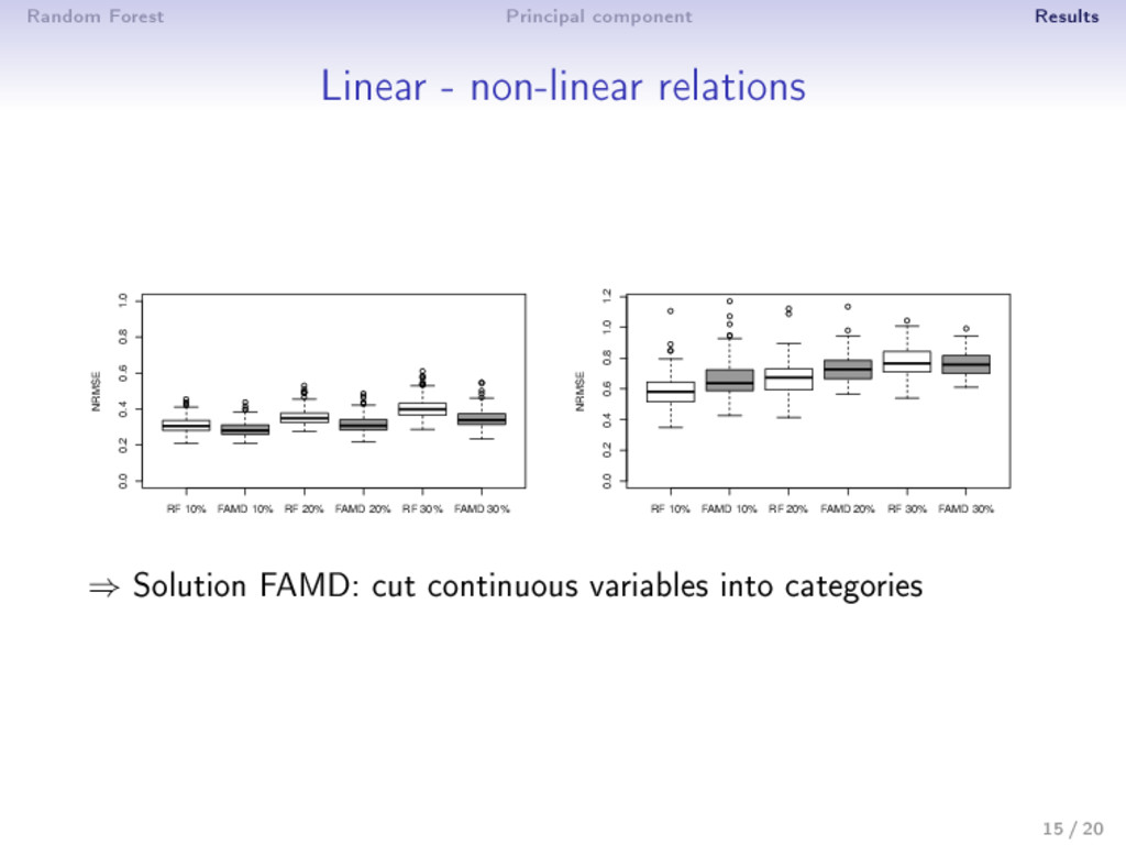
23. Random Forest Principal component Results Iterative FAMD ⇒ Properties: • Imputation based on scores and loadings ⇒ similarities between individuals and relationships between continuous and categorical variables • Linear relationships • Compared to a PCA on the (unweighted) indicator matrix, small categories are better imputed • The number of dimensions is a tuning parameter 13 / 20
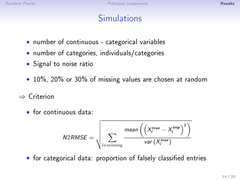
24. Random Forest Principal component Results Simulations • number of continuous - categorical variables • number of categories, individuals/categories • Signal to noise ratio • 10%, 20% or 30% of missing values are chosen at random ⇒ Criterion • for continuous data: N2RMSE = i∈missing mean Xtrue i − Ximp i 2 var (Xtrue i ) • for categorical data: proportion of falsely classied entries 14 / 20
25. Random Forest Principal component Results Linear - non-linear relations q q q q q q q q q q q q q q q q q q q q q q q q q q q q q q q q q q q RF 10% FAMD 10% RF 20% FAMD 20% RF 30% FAMD 30% 0.0 0.2 0.4 0.6 0.8 1.0 NRMSE q q q q q q q q q q q q q q q RF 10% FAMD 10% RF 20% FAMD 20% RF 30% FAMD 30% 0.0 0.2 0.4 0.6 0.8 1.0 1.2 NRMSE ⇒ Solution FAMD: cut continuous variables into categories 15 / 20
26. Random Forest Principal component Results Interactions q q q RF 10% FAMD 10% RF 20% FAMD 20% RF 30% FAMD 30% 0.0 0.2 0.4 0.6 0.8 1.0 1.2 NRMSE q RF 10% FAMD 10% RF 20% FAMD 20% RF 30% FAMD 30% 0.0 0.2 0.4 0.6 0.8 1.0 PFC ⇒ FAMD based on relationships between pairs of variables ⇒ The quality of imputation is poor - close mean imputation ⇒ Solution FAMD: add a variable corresponding to interaction 16 / 20
27. Random Forest Principal component Results Rares categories Number of rows f FAMD Random forest 100 10% 0.060 0.096 100 4% 0.082 0.173 1000 10% 0.042 0.041 1000 4% 0.060 0.071 1000 1% 0.074 0.167 1000 0.4% 0.107 0.241 17 / 20
28. Random Forest Principal component Results Comparison with random forest on real data sets Imputations obtained with random forest & iterative algorithm q q q q q q RF 10% AFDM 10% RF 20% AFDM 20% RF 30% AFDM 30% 2.2 2.4 2.6 2.8 GBSG2 N2RMSE q q RF 10% AFDM 10% RF 20% AFDM 20% RF 30% AFDM 30% 0.25 0.30 0.35 PFC 18 / 20
29. Random Forest Principal component Results Comparison with random forest on real data sets Imputations obtained with random forest & iterative algorithm q q q q q q RF 10% AFDM 10% RF 20% AFDM 20% RF 30% AFDM 30% 2.2 2.4 2.6 2.8 GBSG2 N2RMSE q q RF 10% AFDM 10% RF 20% AFDM 20% RF 30% AFDM 30% 0.25 0.30 0.35 PFC q RF 10% AFDM 10% RF 20% AFDM 20% RF 30% AFDM 30% 1.6 1.8 2.0 2.2 2.4 Ozone N2RMSE q RF 10% AFDM 10% RF 20% AFDM 20% RF 30% AFDM 30% 0.2 0.3 0.4 0.5 PFC 18 / 20
30. Random Forest Principal component Results Conclusion Random Forests: • non-linear relationships between continuous variables • interactions ⇒ no tuning parameters? ⇒ package missForest Principal component: • linear relationships • categorical variables especially rare categories ⇒ tuning parameters: number of dimensions, cv? approximation? ⇒ package missMDA: • handles missing values in PC methods (PCA, MCA, FAMD, MFA) • impute continuous, categorical and mixed data 19 / 20
31. Random Forest Principal component Results Perspectives How to perform a statistical analysis from an incomplete dataset? • we can modify the estimation process to apply it on an incomplete dataset (not always easy!) • we can predict the missing entries with a single imputation method, but BE CAREFUL using the usual methods leads to underestimate the standard errors ⇒ An alternative is to use multiple imputation ... and single imputation is a rst step towards multiple imputation 20 / 20