visualization: • Principal Component Analysis ⇒ continuous variables • Correspondence Analysis ⇒ contingency table • Multiple Correspondence Analysis ⇒ categorical variables ⇒ Dimensionality reduction (describe the data with a smaller number of variables) ⇒ Geometrical approach: importance to graphical displays ⇒ No probabilistic framework, in line with Benzecri (1973)’s idea: “Let the data speak for themselves” 3 / 35
with specific row and column weights and metrics (used to compute the distances). “Doing a data analysis, in good mathematics, is simply searching eigenvectors, all the science of it (the art) is just to find the right matrix to diagonalize. (Benzecri, 1973)” ⇒ Specific choices of weights and metrics can be viewed as inducing specific models for the data under analysis. ⇒ Understanding the connections between exploratory multivariate methods and their cognate models (selecting number of PC, missing values; estimation with SVD, graphics, etc..) 4 / 35
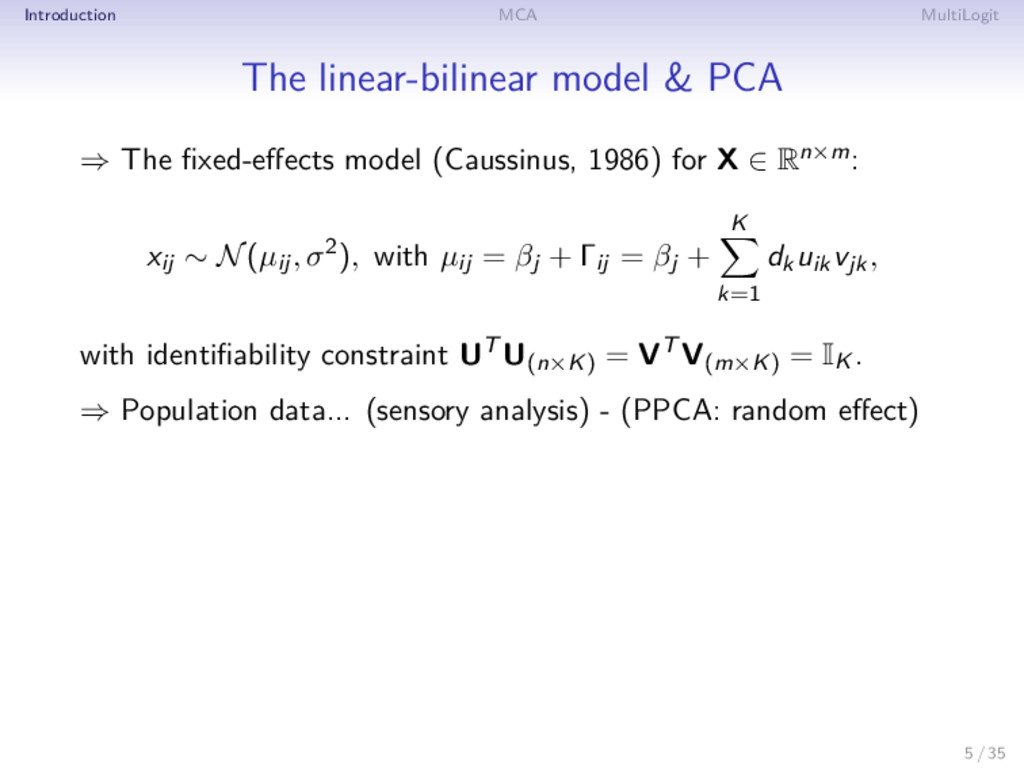
fixed-effects model (Caussinus, 1986) for X ∈ Rn×m: xij ∼ N(µij, σ2), with µij = βj + Γij = βj + K k=1 dkuikvjk, with identifiability constraint UT U(n×K) = VT V(m×K) = IK . ⇒ Population data... (sensory analysis) - (PPCA: random effect) 5 / 35
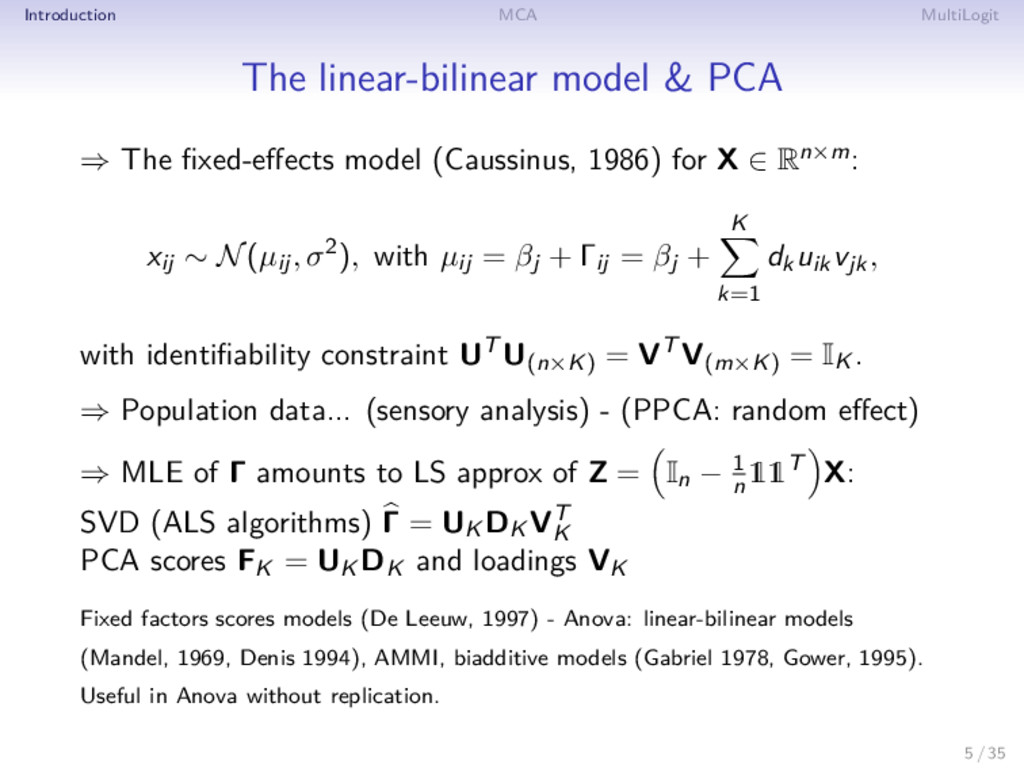
fixed-effects model (Caussinus, 1986) for X ∈ Rn×m: xij ∼ N(µij, σ2), with µij = βj + Γij = βj + K k=1 dkuikvjk, with identifiability constraint UT U(n×K) = VT V(m×K) = IK . ⇒ Population data... (sensory analysis) - (PPCA: random effect) ⇒ MLE of Γ amounts to LS approx of Z = In − 1 n 11T X: SVD (ALS algorithms) Γ = UK DK VT K PCA scores FK = UK DK and loadings VK Fixed factors scores models (De Leeuw, 1997) - Anova: linear-bilinear models (Mandel, 1969, Denis 1994), AMMI, biadditive models (Gabriel 1978, Gower, 1995). Useful in Anova without replication. 5 / 35
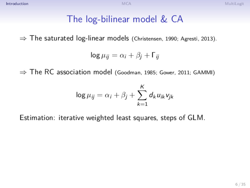
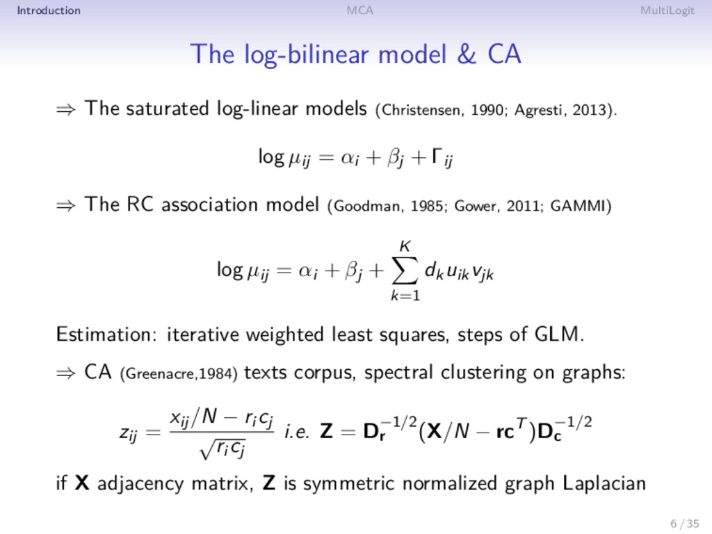
saturated log-linear models (Christensen, 1990; Agresti, 2013). log µij = αi + βj + Γij ⇒ The RC association model (Goodman, 1985; Gower, 2011; GAMMI) log µij = αi + βj + K k=1 dkuikvjk Estimation: iterative weighted least squares, steps of GLM. ⇒ CA (Greenacre,1984) texts corpus, spectral clustering on graphs: zij = xij/N − ri cj √ ri cj i.e. Z = D−1/2 r (X/N − rcT )D−1/2 c if X adjacency matrix, Z is symmetric normalized graph Laplacian 6 / 35
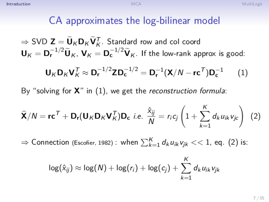
Z = UK DK VT K . Standard row and col coord UK = D−1/2 r UK , VK = D−1/2 c VK . If the low-rank approx is good: UK DK VT K ≈ D−1/2 r ZD−1/2 c = D−1 r (X/N − rcT )D−1 c (1) By “solving for X” in (1), we get the reconstruction formula: X/N = rcT + Dr(UK DK VT K )Dc i.e. ˆ xij N = ri cj 1 + K k=1 dkuikvjc (2) 7 / 35
Z = UK DK VT K . Standard row and col coord UK = D−1/2 r UK , VK = D−1/2 c VK . If the low-rank approx is good: UK DK VT K ≈ D−1/2 r ZD−1/2 c = D−1 r (X/N − rcT )D−1 c (1) By “solving for X” in (1), we get the reconstruction formula: X/N = rcT + Dr(UK DK VT K )Dc i.e. ˆ xij N = ri cj 1 + K k=1 dkuikvjc (2) ⇒ Connection (Escofier, 1982) : when K k=1 dkuikvjk << 1, eq. (2) is: log(ˆ xij) ≈ log(N) + log(ri ) + log(cj) + K k=1 dkuikvjk 7 / 35
in the social sciences • medical research: understand the genetic and environmental risk factors of diseases. Ex diabetes: 300 questions (56 pages of questionnaire!) on the food consumption habits, the previous illness in the family, the presence of animals in the household, the kind of paint used in the rooms, etc. • genetic study: the relationship between a sequence of ACGT nucleotides 9 / 35
mn (A − 1pT )D−1/2 p ΓMCA to be the SVD decomposition UK DK VT K of ZA. Homogeneity Analysis (Gifi 1990, J. de Leeuw, J. Meulman), Dual scaling (Nishisato, 1980, Guttman, 1941) ⇒ Interpreting the graphical displays where rows are represented with F = UKDK and categories with VK = D−1/2 p VK Properties: • Fk = arg maxFk∈Rn m j=1 η2(Fk, Xm) - counterpart of PCA • the distances between the rows and between the columns coincide with the χ2 distances. 12 / 35
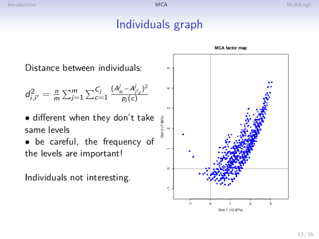
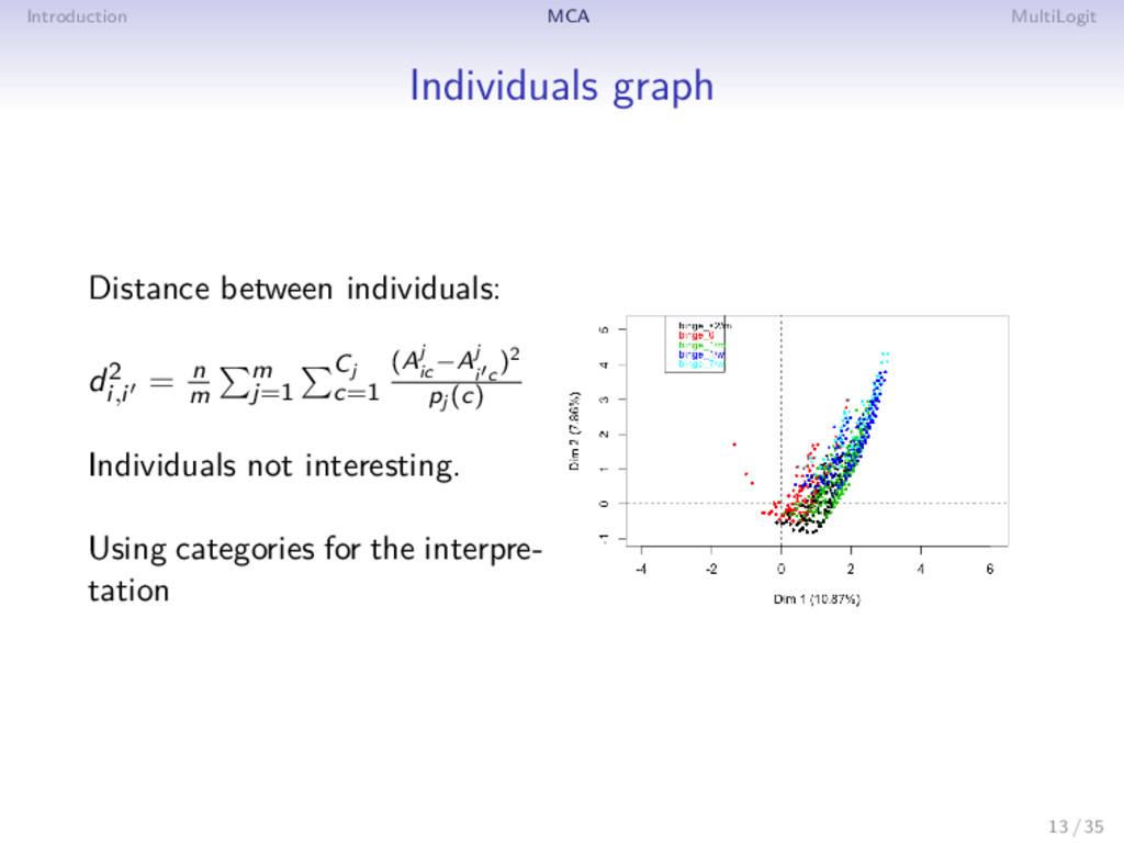
= n m m j=1 Cj c=1 (Aj ic −Aj i c )2 pj (c) • different when they don’t take same levels • be careful, the frequency of the levels are important! Individuals not interesting. −1 0 1 2 3 −1 0 1 2 3 4 5 MCA factor map Dim 1 (10.87%) Dim 2 (7.86%) 13 / 35
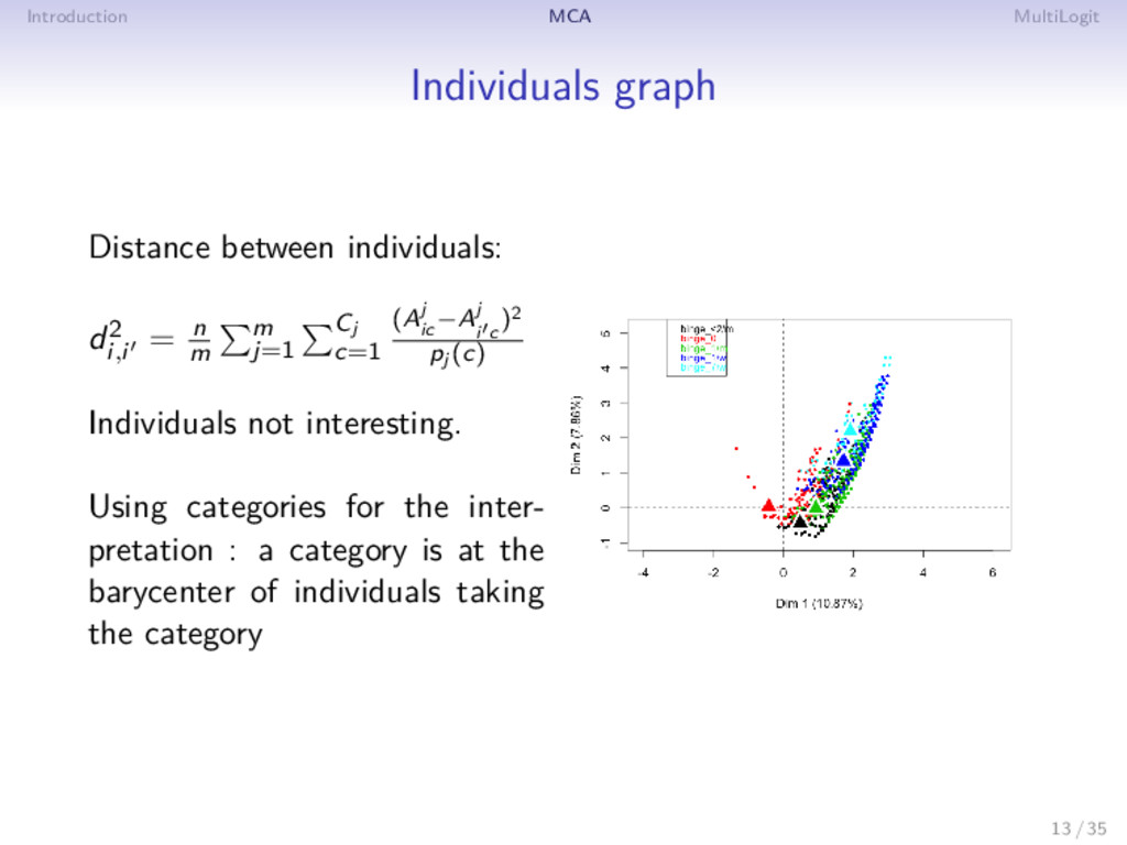
= n m m j=1 Cj c=1 (Aj ic −Aj i c )2 pj (c) Individuals not interesting. Using categories for the inter- pretation : a category is at the barycenter of individuals taking the category 13 / 35
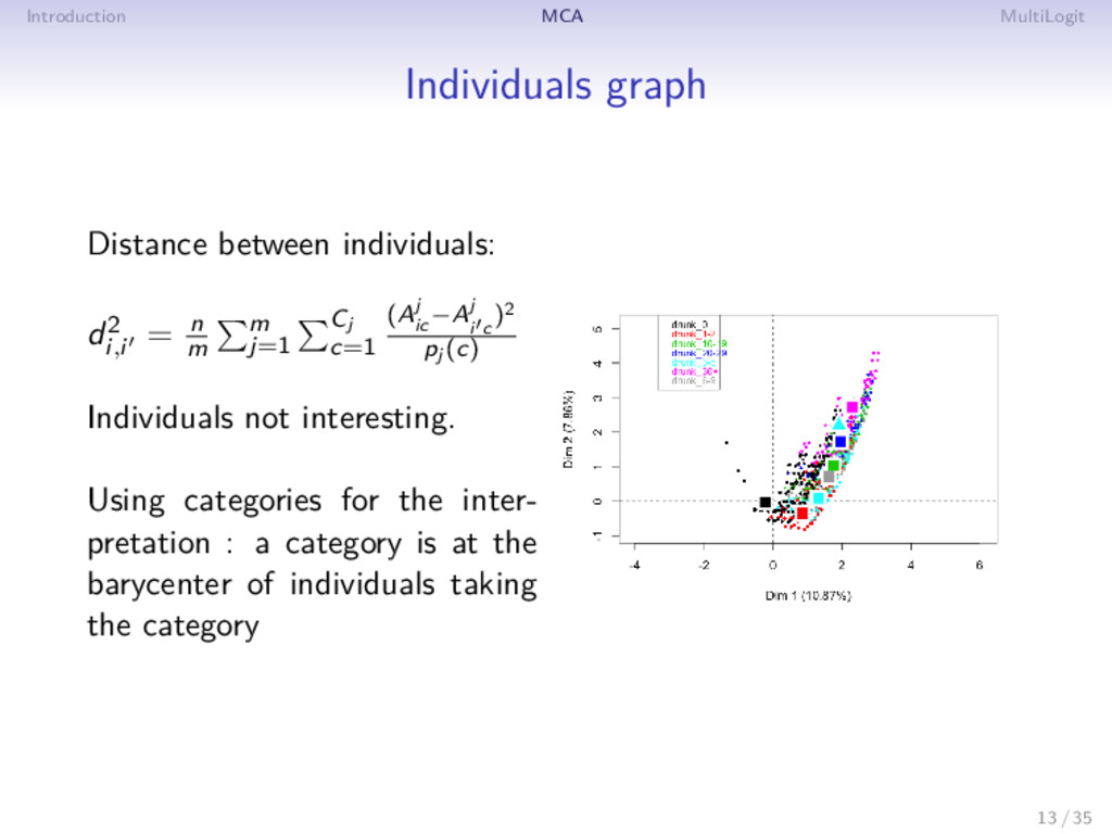
= n m m j=1 Cj c=1 (Aj ic −Aj i c )2 pj (c) Individuals not interesting. Using categories for the inter- pretation : a category is at the barycenter of individuals taking the category 13 / 35
= n m m j=1 Cj c=1 (Aj ic −Aj i c )2 pj (c) Individuals not interesting. Using categories for the inter- pretation : a category is at the barycenter of individuals taking the category 13 / 35
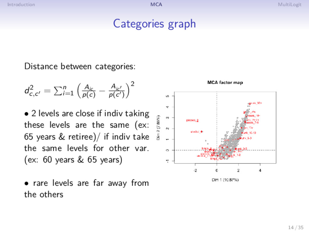
= n i=1 Aic p(c) − Aic p(c ) 2 • 2 levels are close if indiv taking these levels are the same (ex: 65 years & retiree)/ if indiv take the same levels for other var. (ex: 60 years & 65 years) • rare levels are far away from the others 14 / 35
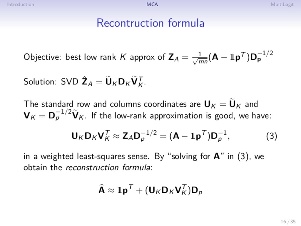
approx of ZA = 1 √ mn (A − 1pT )D−1/2 p Solution: SVD ˆ ZA = UK DK VT K . The standard row and columns coordinates are UK = UK and VK = D−1/2 p VK . If the low-rank approximation is good, we have: UK DK VT K ≈ ZAD−1/2 p = (A − 1pT )D−1 p , (3) in a weighted least-squares sense. By “solving for A” in (3), we obtain the reconstruction formula: A ≈ 1pT + (UK DK VT K )Dp 16 / 35
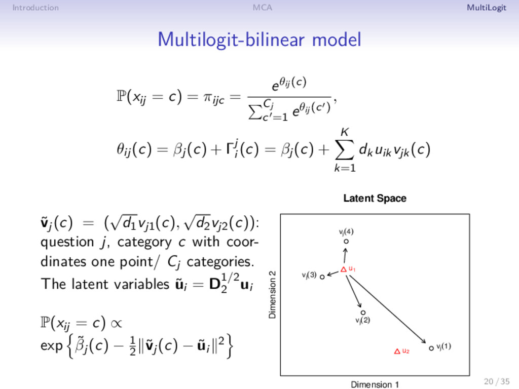
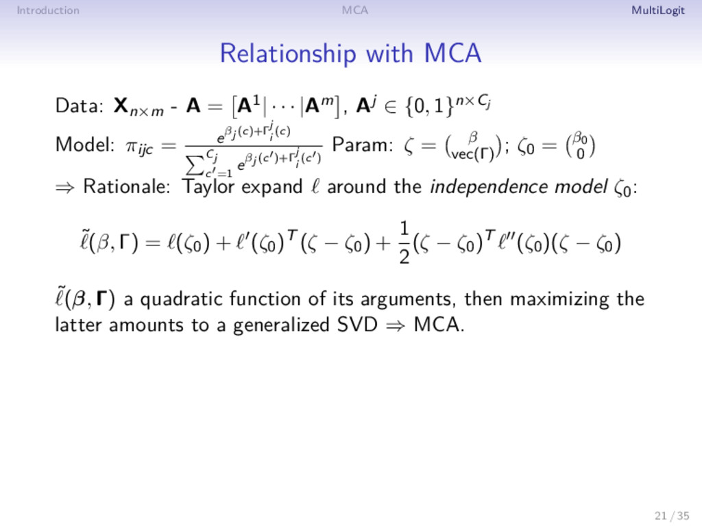
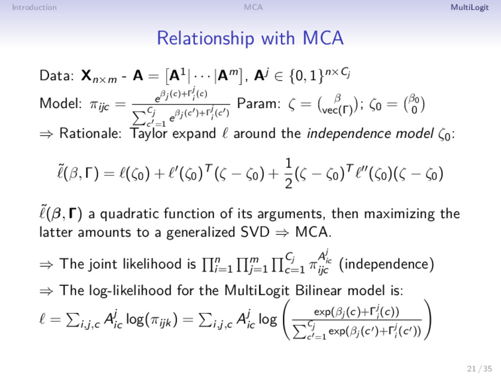
= A1| · · · |Am , Aj ∈ {0, 1}n×Cj Model: πijc = eβj (c)+Γ j i (c) Cj c =1 eβj (c )+Γ j i (c ) Param: ζ = β vec(Γ) ; ζ0 = β0 0 ⇒ Rationale: Taylor expand around the independence model ζ0: ˜(β, Γ) = (ζ0) + (ζ0)T (ζ − ζ0) + 1 2 (ζ − ζ0)T (ζ0)(ζ − ζ0) ˜(β, Γ) a quadratic function of its arguments, then maximizing the latter amounts to a generalized SVD ⇒ MCA. ⇒ The joint likelihood is n i=1 m j=1 Cj c=1 πAj ic ijc (independence) ⇒ The log-likelihood for the MultiLogit Bilinear model is: = i,j,c Aj ic log(πijk) = i,j,c Aj ic log exp(βj (c)+Γj i (c)) Cj c =1 exp(βj (c )+Γj i (c )) 21 / 35
βj(Aj i ) + Γj i (Aj i ) − log Cj c=1 eβj (c)+Γj i (c) ∂ ∂Γj i (c) = 1xij =c − eβj (c)+Γj i (c) Cj c =1 eβj (c )+Γj i (c ) = Aj ic − πijc (4) ∂ ∂Γj i (c)∂Γj i (c ) = πijcπijc − πijc1c=c j = j , i = i 0 o.w. (5) Evaluating (4) at ζ0 = (β0 = log(p), 0) gives Aj ic − pj(c) - idem (5) ˜(β, Γ) ≈ Γ, A − 1pT − 1 2 ΓD1/2 p 2 F 22 / 35
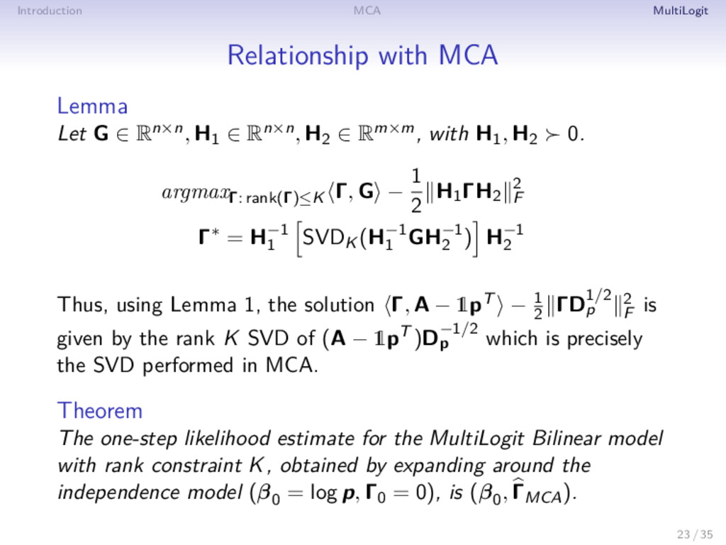
Rn×n, H1 ∈ Rn×n, H2 ∈ Rm×m, with H1, H2 0. argmaxΓ: rank(Γ)≤K Γ, G − 1 2 H1ΓH2 2 F Γ∗ = H−1 1 SVDK (H−1 1 GH−1 2 ) H−1 2 Thus, using Lemma 1, the solution Γ, A − 1pT − 1 2 ΓD1/2 p 2 F is given by the rank K SVD of (A − 1pT )D−1/2 p which is precisely the SVD performed in MCA. Theorem The one-step likelihood estimate for the MultiLogit Bilinear model with rank constraint K, obtained by expanding around the independence model (β0 = log p, Γ0 = 0), is (β0 , ΓMCA). 23 / 35
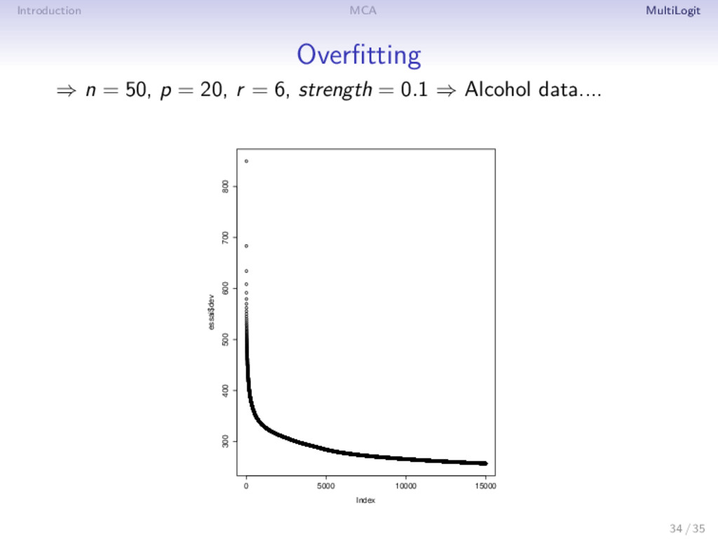
. . . , Am] Model: πijc = exp(θij(c) ) Cj c =1 exp(θij(c ) ) θij(c) = βj(c) + K k=1 dkuikvjk(c) Identification constraint: βj 1 = 0, 1 U = 0, U U = I, 1 Vj = 0 Maximum dimensionality: K = min(n − 1, m j=1 Cj − m) Estimation: MLE ⇒ Problem: overfitting: θij(c) → ∞ or θij(c) → −∞ ⇒ Solution: penalized likelihood. L(β, U, D, V) = − n i=1 m j=1 Cj c=1 Aj ic log(πijc) + λ K k=1 dk 24 / 35
Leeuw & Heiser, 1977; Lange, 2004) use in each iteration a majorizing function g(θ, θ0). • Current estimate θ0 is called supporting point. • Requirements: 1 f (θ0 ) = g(θ0, θ0 ). 2 f (θ) ≤ g(θ, θ0 ). • Sandwich inequality: f (θ+) ≤ g(θ+, θ0) ≤ g(θ0, θ0) = f (θ0) with θ+ = argming(θ, θ0) • Any majorization algorithm is guaranteed to descent. 25 / 35
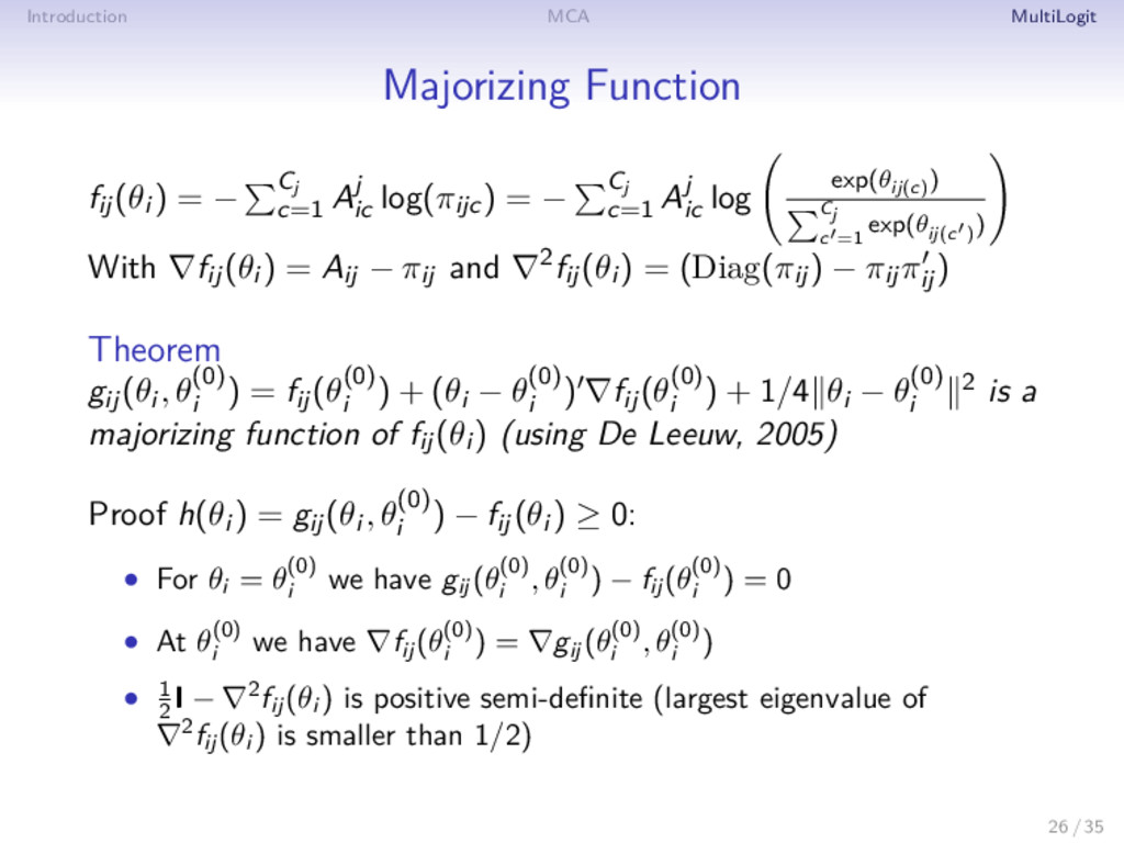
c=1 Aj ic log(πijc) = − Cj c=1 Aj ic log exp(θij(c) ) Cj c =1 exp(θij(c ) ) With ∇fij(θi ) = Aij − πij and ∇2fij(θi ) = (Diag(πij) − πijπij ) Theorem gij(θi , θ(0) i ) = fij(θ(0) i ) + (θi − θ(0) i ) ∇fij(θ(0) i ) + 1/4 θi − θ(0) i 2 is a majorizing function of fij(θi ) (using De Leeuw, 2005) Proof h(θi ) = gij(θi , θ(0) i ) − fij(θi ) ≥ 0: • For θi = θ(0) i we have gij (θ(0) i , θ(0) i ) − fij (θ(0) i ) = 0 • At θ(0) i we have ∇fij (θ(0) i ) = ∇gij (θ(0) i , θ(0) i ) • 1 2 I − ∇2fij (θi ) is positive semi-definite (largest eigenvalue of ∇2fij (θi ) is smaller than 1/2) 26 / 35
c=1 Aj ic log(πijc) = − Cj c=1 Aj ic log exp(θij(c) ) Cj c =1 exp(θij(c ) ) With ∇fij(θi ) = Aij − πij and ∇2fij(θi ) = (Diag(πij) − πijπij ) Theorem gij(θi , θ(0) i ) = fij(θ(0) i ) + (θi − θ(0) i ) ∇fij(θ(0) i ) + 1/4 θi − θ(0) i 2 is a majorizing function of fij(θi ) (using De Leeuw, 2005) Proof h(θi ) = gij(θi , θ(0) i ) − fij(θi ) ≥ 0: • For θi = θ(0) i we have gij (θ(0) i , θ(0) i ) − fij (θ(0) i ) = 0 • At θ(0) i we have ∇fij (θ(0) i ) = ∇gij (θ(0) i , θ(0) i ) • 1 2 I − ∇2fij (θi ) is positive semi-definite (largest eigenvalue of ∇2fij (θi ) is smaller than 1/2) 26 / 35
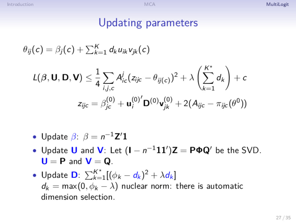
k=1 dkuikvjk(c) L(β, U, D, V) ≤ 1 4 i,j,c Aj ic (zijc − θij(c) )2 + λ K k=1 dk + c zijc = β(0) jc + u(0) i D(0)v(0) jk + 2(Aijc − πijc(θ0)) • Update β: β = n−1Z 1 • Update U and V: Let (I − n−111 )Z = PΦQ be the SVD. U = P and V = Q. • Update D: K k=1 [(φk − dk)2 + λdk] dk = max(0, φk − λ) nuclear norm: there is automatic dimension selection. 27 / 35
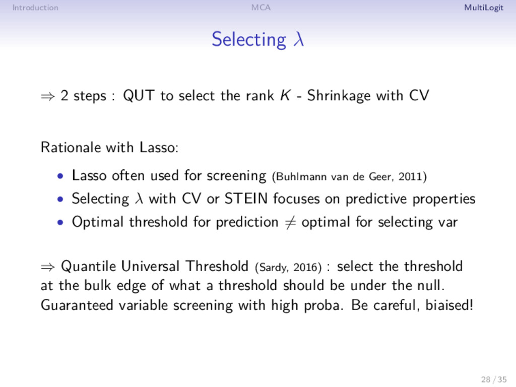
to select the rank K - Shrinkage with CV Rationale with Lasso: • Lasso often used for screening (Buhlmann van de Geer, 2011) • Selecting λ with CV or STEIN focuses on predictive properties • Optimal threshold for prediction = optimal for selecting var ⇒ Quantile Universal Threshold (Sardy, 2016) : select the threshold at the bulk edge of what a threshold should be under the null. Guaranteed variable screening with high proba. Be careful, biaised! 28 / 35
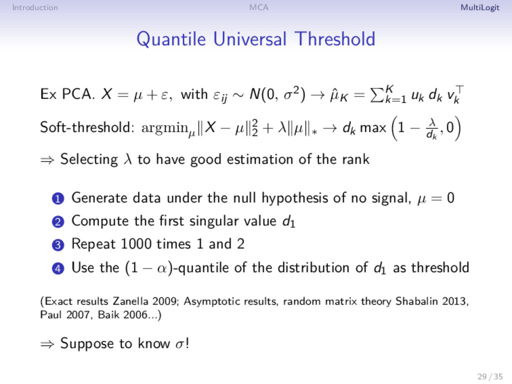
µ + ε, with εij ∼ N(0, σ2) → ˆ µK = K k=1 uk dk vk Soft-threshold: argminµ X − µ 2 2 + λ µ ∗ → dk max 1 − λ dk , 0 ⇒ Selecting λ to have good estimation of the rank 1 Generate data under the null hypothesis of no signal, µ = 0 2 Compute the first singular value d1 3 Repeat 1000 times 1 and 2 4 Use the (1 − α)-quantile of the distribution of d1 as threshold (Exact results Zanella 2009; Asymptotic results, random matrix theory Shabalin 2013, Paul 2007, Baik 2006...) ⇒ Suppose to know σ! 29 / 35
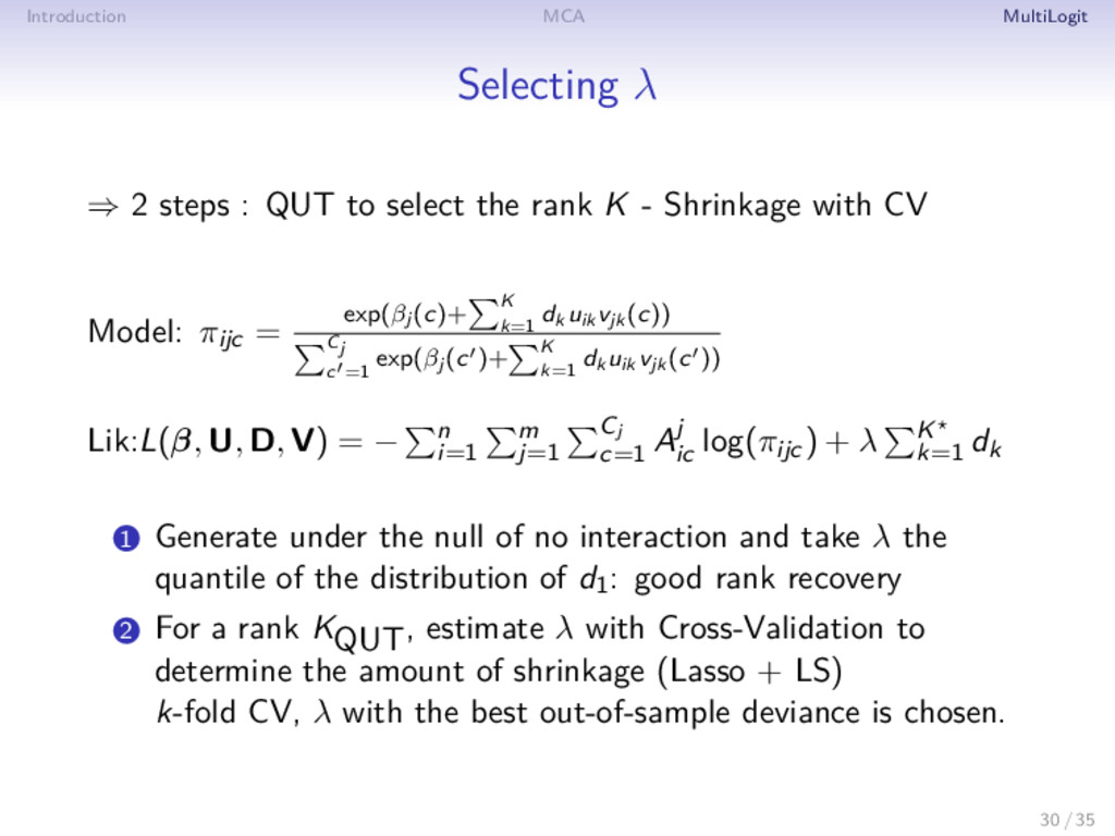
to select the rank K - Shrinkage with CV Model: πijc = exp(βj (c)+ K k=1 dk uik vjk (c)) Cj c =1 exp(βj (c )+ K k=1 dk uik vjk (c )) Lik:L(β, U, D, V) = − n i=1 m j=1 Cj c=1 Aj ic log(πijc) + λ K k=1 dk 1 Generate under the null of no interaction and take λ the quantile of the distribution of d1: good rank recovery 2 For a rank KQUT, estimate λ with Cross-Validation to determine the amount of shrinkage (Lasso + LS) k-fold CV, λ with the best out-of-sample deviance is chosen. 30 / 35
linearized estimate of the parameters of the multinomial logit bilinear model ⇒ MCA a proxy to estimate the model’s parameters (small interaction) • graphics • mixed data (quanti, quali) - FAMD / Multiple Factor Analysis for groups of variables • mixture of MCA/ mixture of PPCA • selecting the rank with BIC?? Fixed effect, asymptotics, n - p? • regularization in MCA to tackle overfitting issues • missing values 35 / 35