Multiple imputation Practice Appendix Outline 1 Introduction 2 Point estimates of the PCA axes and components 3 Uncertainty 4 MCA/MFA 5 Single imputation for mixed variables 6 Multiple imputation 7 Practice 8 Appendix 2 / 92
Multiple imputation Practice Appendix Missing values Gertrude Mary Cox “The best thing to do with missing values is not to have any” Missing values are ubiquitous: • no answer in a questionnaire • data that are lost or destroyed • machines that fail • plants damaged • ... Still an issue in the "big data" area 3 / 92
Multiple imputation Practice Appendix Some references Schafer (1997) Little & Rubin (1987, 2002) Joseph L. Schafer Roderick Little Donald Rubin Suggested reading: chap 25 of Gelman & Hill (2006) Andrew Gelman Jennifer L. Hill 4 / 92
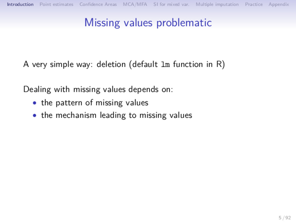
Multiple imputation Practice Appendix Missing values problematic A very simple way: deletion (default lm function in R) Dealing with missing values depends on: • the pattern of missing values • the mechanism leading to missing values 5 / 92
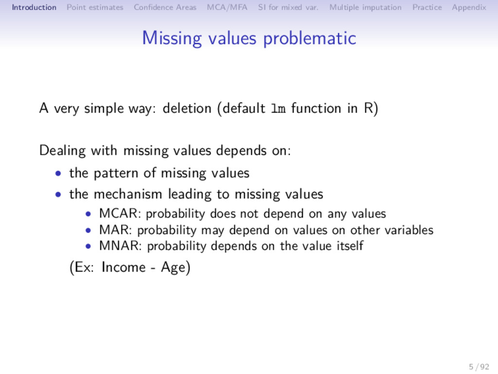
Multiple imputation Practice Appendix Missing values problematic A very simple way: deletion (default lm function in R) Dealing with missing values depends on: • the pattern of missing values • the mechanism leading to missing values • MCAR: probability does not depend on any values • MAR: probability may depend on values on other variables • MNAR: probability depends on the value itself (Ex: Income - Age) 5 / 92
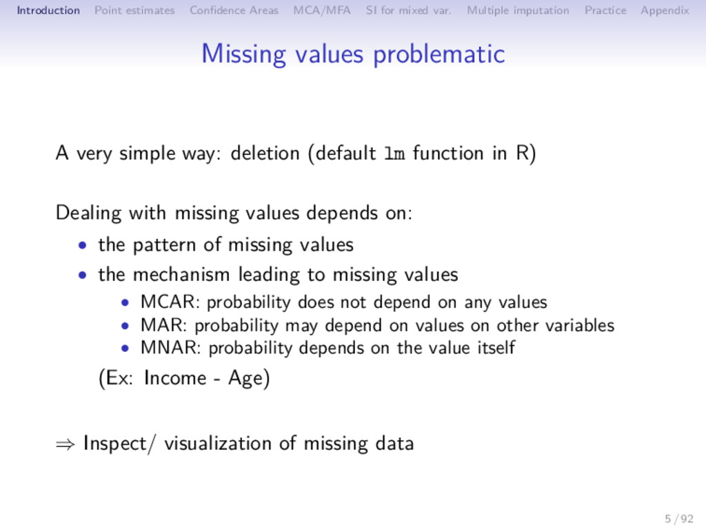
Multiple imputation Practice Appendix Missing values problematic A very simple way: deletion (default lm function in R) Dealing with missing values depends on: • the pattern of missing values • the mechanism leading to missing values • MCAR: probability does not depend on any values • MAR: probability may depend on values on other variables • MNAR: probability depends on the value itself (Ex: Income - Age) ⇒ Inspect/ visualization of missing data 5 / 92
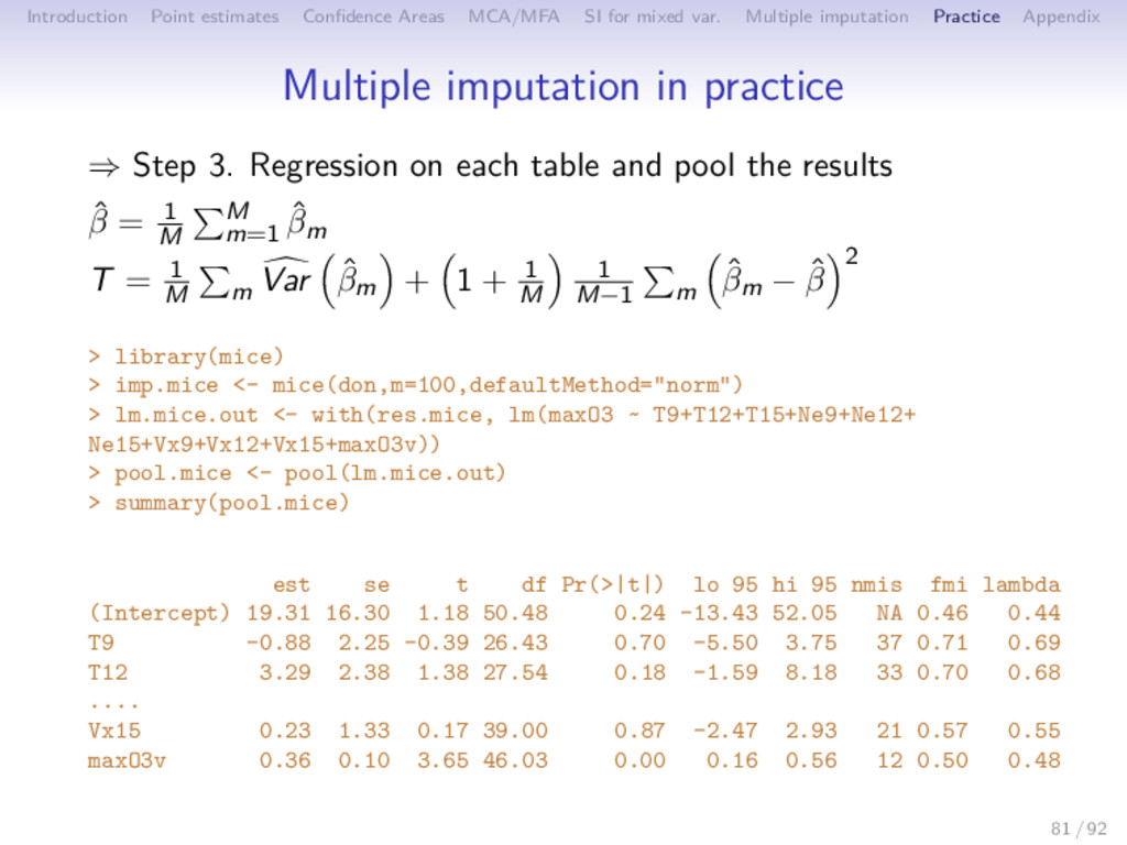
Multiple imputation Practice Appendix Recommended methods ⇒ Multiple imputation (Rubin, 1987) • Generate M plausible values for each missing value ( ˆ F ˆ u′)ij ( ˆ F ˆ u′)1 ij + ε1 ij ( ˆ F ˆ u′)2 ij + ε2 ij ( ˆ F ˆ u′)3 ij + ε3 ij ( ˆ F ˆ u′)B ij + εB ij • Perform the analysis on each imputed data set: ˆ θm, Var ˆ θm • Combine the results: ˆ θ = 1 M M m=1 ˆ θm T = 1 M M m=1 Var ˆ θm + 1 + 1 M 1 M−1 M m=1 ˆ θm − ˆ θ 2 7 / 92
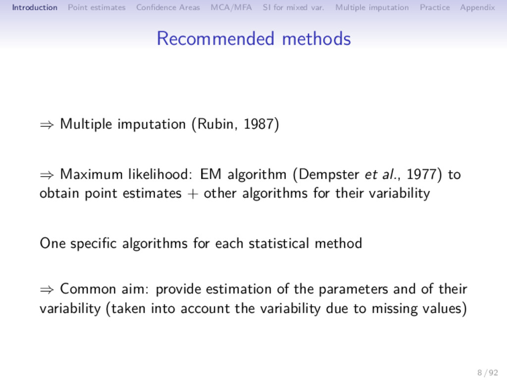
Multiple imputation Practice Appendix Recommended methods ⇒ Multiple imputation (Rubin, 1987) ⇒ Maximum likelihood: EM algorithm (Dempster et al., 1977) to obtain point estimates + other algorithms for their variability One specific algorithms for each statistical method ⇒ Common aim: provide estimation of the parameters and of their variability (taken into account the variability due to missing values) 8 / 92
Multiple imputation Practice Appendix Outline 1 Introduction 2 Point estimates of the PCA axes and components 3 Uncertainty 4 MCA/MFA 5 Single imputation for mixed variables 6 Multiple imputation 7 Practice 8 Appendix 9 / 92
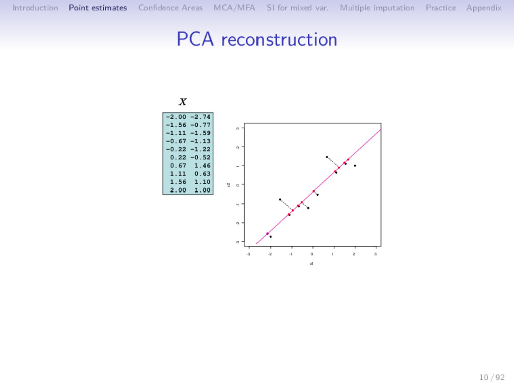
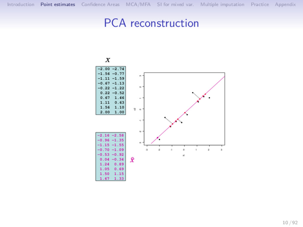
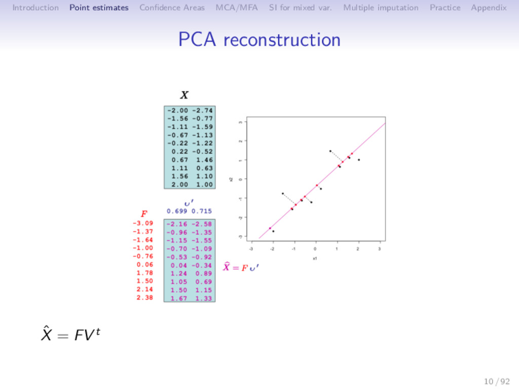
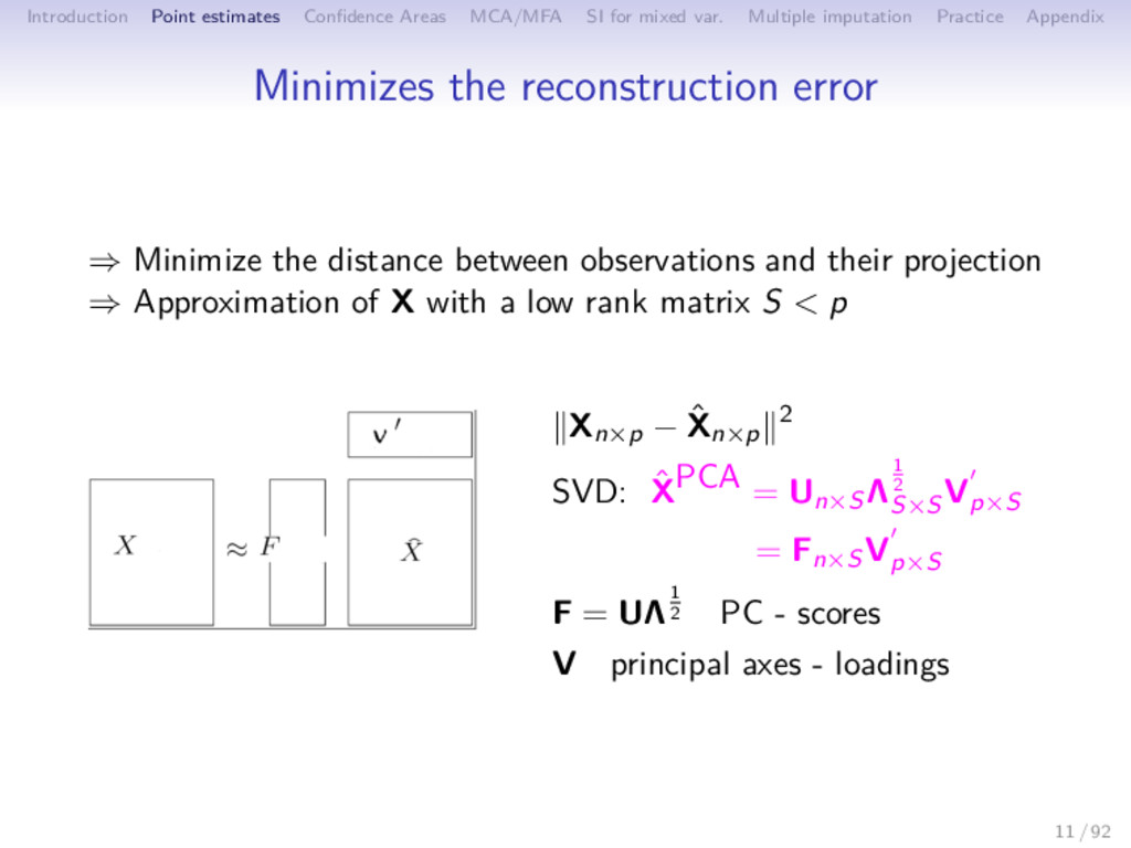
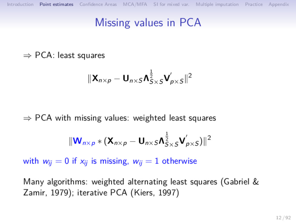
Multiple imputation Practice Appendix Minimizes the reconstruction error ⇒ Minimize the distance between observations and their projection ⇒ Approximation of X with a low rank matrix S < p Xn×p − ˆ Xn×p 2 SVD: ˆ XPCA = Un×SΛ 1 2 S×S Vp×S = Fn×SVp×S F = UΛ1 2 PC - scores V principal axes - loadings 11 / 92
Multiple imputation Practice Appendix Weighted least squares ⇒ Rank 1: n i=1 p j=1 (xij − Fi1Vj1)2 2 simple regressions: Vj1 = i (xij ×Fi1) i F2 i1 Fi1 = j (xij ×Vj1) j u2 j1 Power method. Deflation: (F2, V2) in ˆ ε1 = X − F1V1 NIPALS (Non linear Iterative PArtial Least Squares, Wold, Christofferson, 1966, 1969). Vj1 = i (wij xij Fi1) i wij F2 i1 ; Fi1 = j (wij xij uj1) j wij V 2 j1 ⇒ Subspace S > 1: 2 multiple regressions: V = X F(F F)−1; F = XV (V V )−1 2 multiple weighted regressions 13 / 92
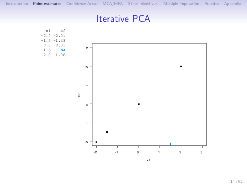
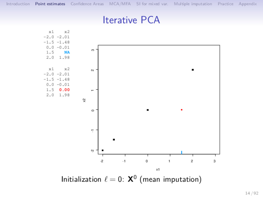
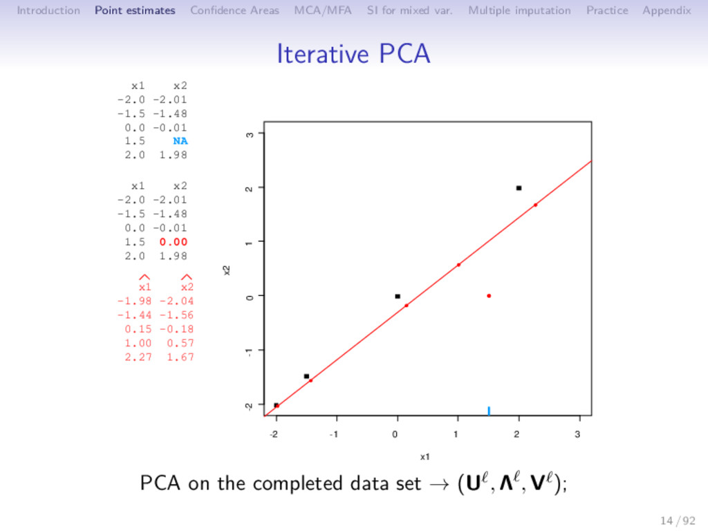
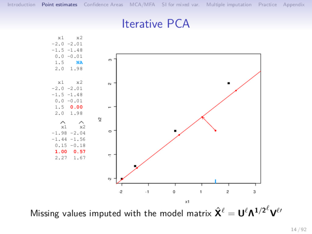
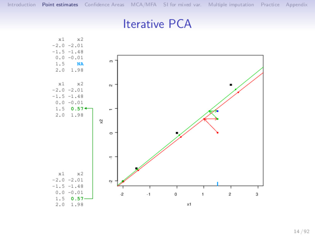
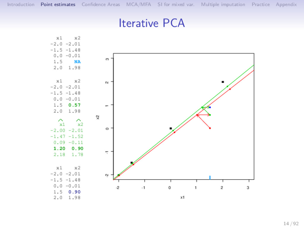
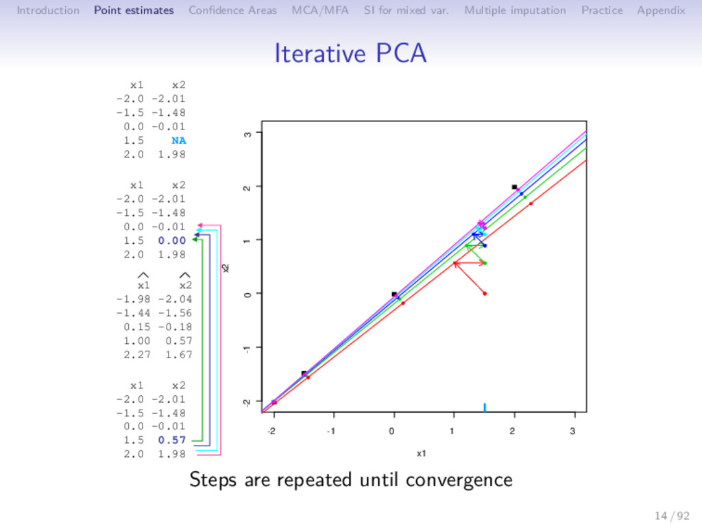
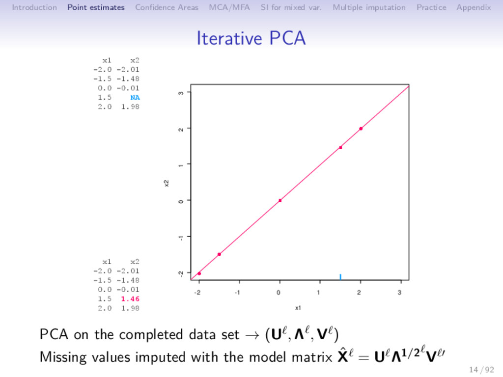
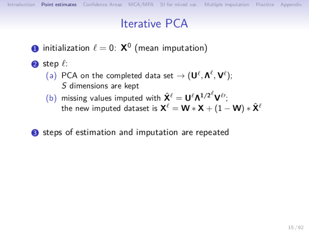
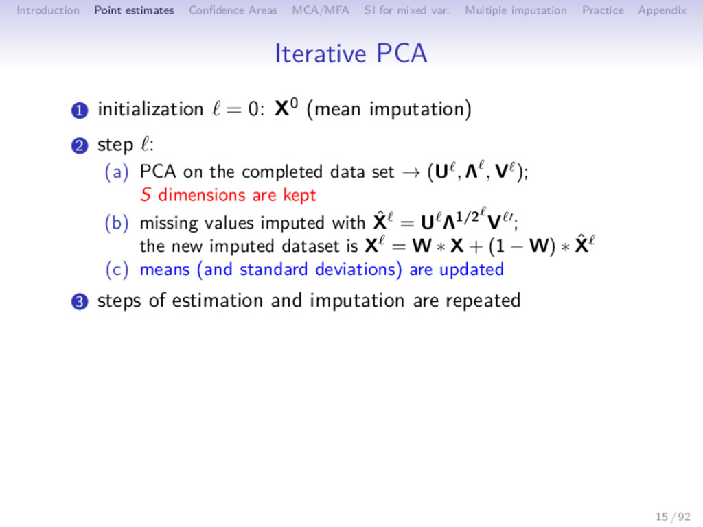
Multiple imputation Practice Appendix Iterative PCA 1 initialization = 0: X0 (mean imputation) 2 step : (a) PCA on the completed data set → (U , Λ , V ); S dimensions are kept (b) missing values imputed with ˆ X = U Λ1/2 V ; the new imputed dataset is X = W ∗ X + (1 − W) ∗ ˆ X 3 steps of estimation and imputation are repeated 15 / 92
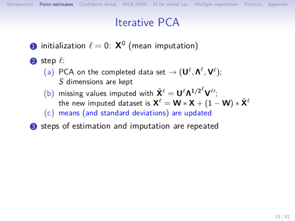
Multiple imputation Practice Appendix Iterative PCA 1 initialization = 0: X0 (mean imputation) 2 step : (a) PCA on the completed data set → (U , Λ , V ); S dimensions are kept (b) missing values imputed with ˆ X = U Λ1/2 V ; the new imputed dataset is X = W ∗ X + (1 − W) ∗ ˆ X (c) means (and standard deviations) are updated 3 steps of estimation and imputation are repeated 15 / 92
Multiple imputation Practice Appendix Iterative PCA 1 initialization = 0: X0 (mean imputation) 2 step : (a) PCA on the completed data set → (U , Λ , V ); S dimensions are kept (b) missing values imputed with ˆ X = U Λ1/2 V ; the new imputed dataset is X = W ∗ X + (1 − W) ∗ ˆ X (c) means (and standard deviations) are updated 3 steps of estimation and imputation are repeated 15 / 92
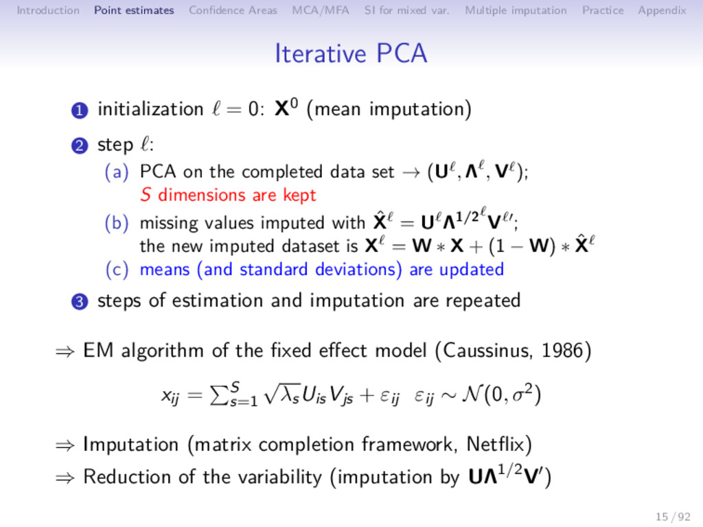
Multiple imputation Practice Appendix Iterative PCA 1 initialization = 0: X0 (mean imputation) 2 step : (a) PCA on the completed data set → (U , Λ , V ); S dimensions are kept (b) missing values imputed with ˆ X = U Λ1/2 V ; the new imputed dataset is X = W ∗ X + (1 − W) ∗ ˆ X (c) means (and standard deviations) are updated 3 steps of estimation and imputation are repeated ⇒ EM algorithm of the fixed effect model (Caussinus, 1986) xij = S s=1 √ λsUisVjs + εij εij ∼ N(0, σ2) ⇒ Imputation (matrix completion framework, Netflix) ⇒ Reduction of the variability (imputation by UΛ1/2V ) 15 / 92
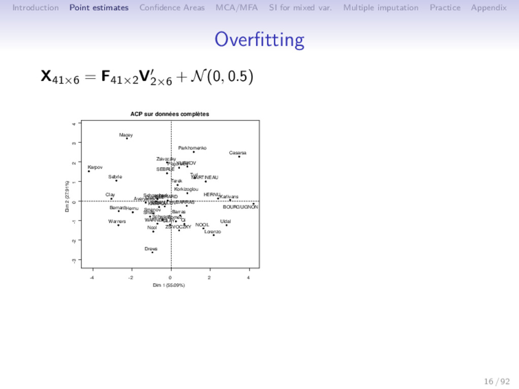
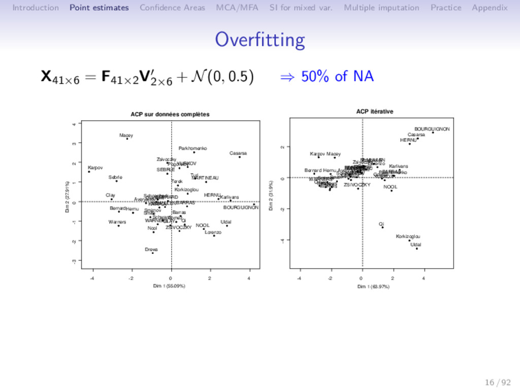
Multiple imputation Practice Appendix Overfitting Overfitting when: • many parameters / the number of observed values (the number of dimensions S and of missing values are important) • data are very noisy ⇒ Trust too much the relationship between variables Remarks: • missing values: special case of small data set • iterative PCA: prediction method Solution: ⇒ Shrinkage methods 17 / 92
Multiple imputation Practice Appendix Properties ⇒ Quality of estimation of the parameters: Simulation X = FV + ε RV coefficient between complete/ incomplete • performances decrease with missing values and level of noise • difficult settings: regularized PCA equals mean imputation • the choice of the number of dimensions is less crucial ⇒ Quality of imputation: • Good when the structure is strong (imputation uses similarities between individuals and relationship between variables) • Competitive with random forests 20 / 92
Multiple imputation Practice Appendix Outline 1 Introduction 2 Point estimates of the PCA axes and components 3 Uncertainty 4 MCA/MFA 5 Single imputation for mixed variables 6 Multiple imputation 7 Practice 8 Appendix 23 / 92
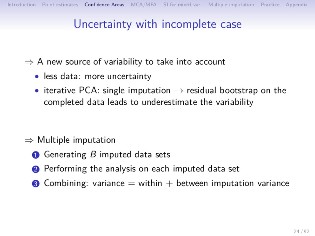
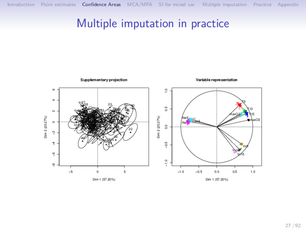
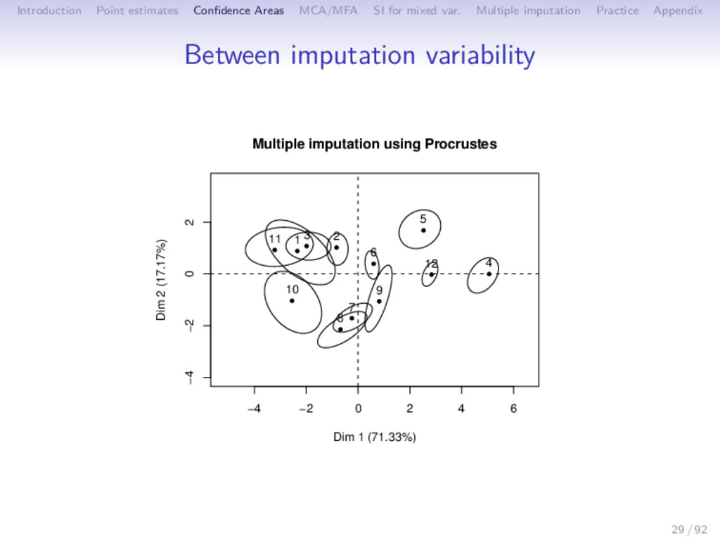
Multiple imputation Practice Appendix Uncertainty with incomplete case ⇒ A new source of variability to take into account • less data: more uncertainty • iterative PCA: single imputation → residual bootstrap on the completed data leads to underestimate the variability ⇒ Multiple imputation 1 Generating B imputed data sets 2 Performing the analysis on each imputed data set 3 Combining: variance = within + between imputation variance 24 / 92
Multiple imputation Practice Appendix Uncertainty with incomplete case ⇒ A new source of variability to take into account • less data: more uncertainty • iterative PCA: single imputation → residual bootstrap on the completed data leads to underestimate the variability ⇒ Multiple imputation 1 Generating B imputed data sets: b = 1, ..., B, missing values xb ij drawn from the predictive N (FV )ij, ˆ σ2 ⇒ "improper" imputation 2 Performing the analysis on each imputed data set 3 Combining: variance = within + between imputation variance 24 / 92
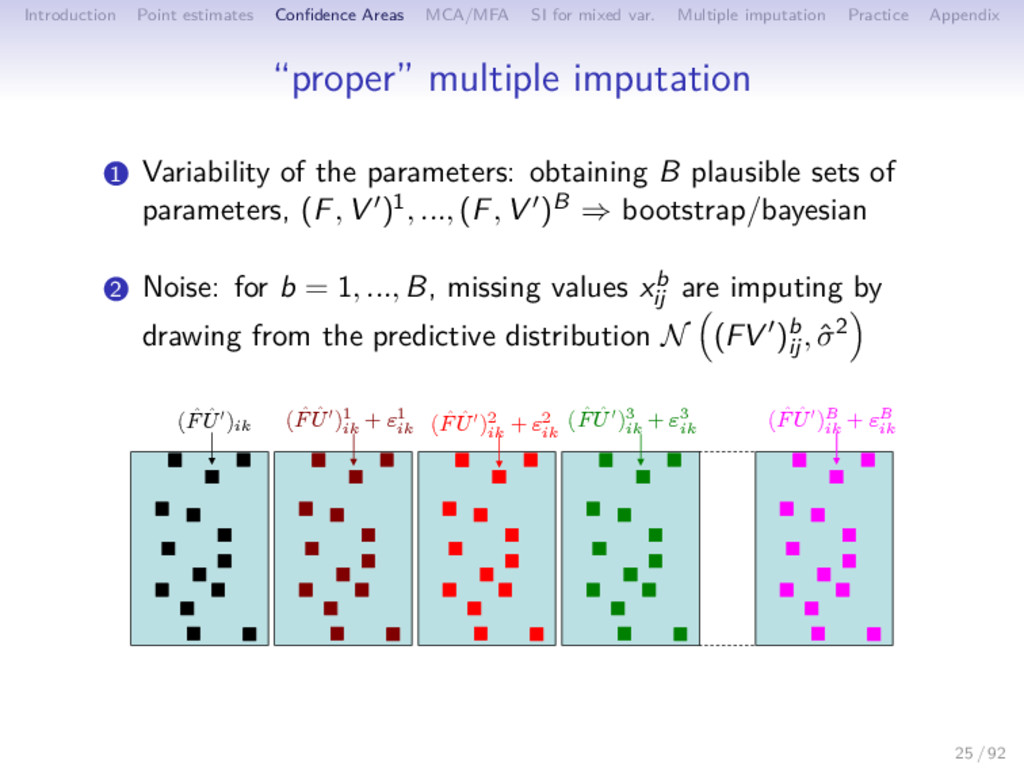
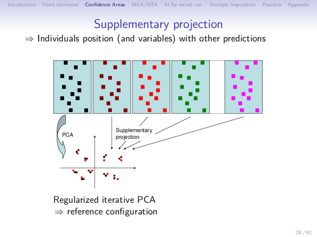
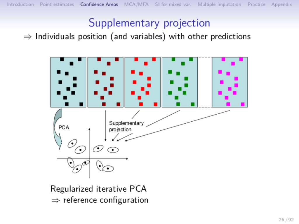
Multiple imputation Practice Appendix “proper” multiple imputation 1 Variability of the parameters: obtaining B plausible sets of parameters, (F, V )1, ..., (F, V )B ⇒ bootstrap/bayesian 2 Noise: for b = 1, ..., B, missing values xb ij are imputing by drawing from the predictive distribution N (FV )b ij , ˆ σ2 ( ˆ F ˆ U′)ik ( ˆ F ˆ U′)1 ik + ε1 ik ( ˆ F ˆ U′)2 ik + ε2 ik ( ˆ F ˆ U′)3 ik + ε3 ik ( ˆ F ˆ U′)B ik + εB ik 25 / 92
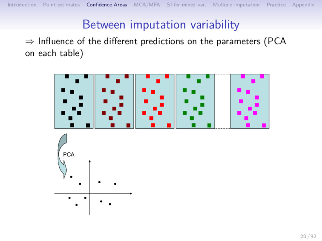
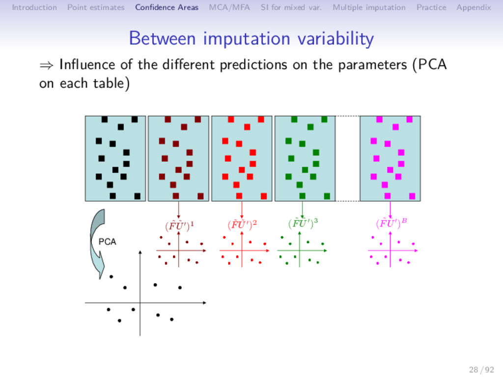
Multiple imputation Practice Appendix Between imputation variability ⇒ Influence of the different predictions on the parameters (PCA on each table) PCA 28 / 92
Multiple imputation Practice Appendix Between imputation variability ⇒ Influence of the different predictions on the parameters (PCA on each table) PCA ( ˜ F ˜ U′)1 ( ˜ F ˜ U′)2 ( ˜ F ˜ U′)3 ( ˜ F ˜ U′)B 28 / 92
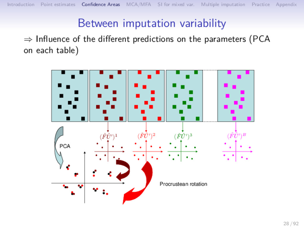
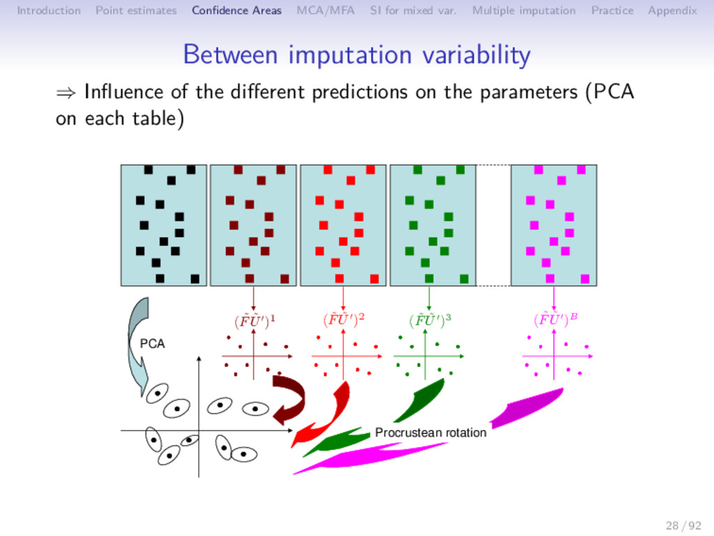
Multiple imputation Practice Appendix Between imputation variability ⇒ Influence of the different predictions on the parameters (PCA on each table) Procrustean rotation PCA ( ˜ F ˜ U′)1 ( ˜ F ˜ U′)2 ( ˜ F ˜ U′)3 ( ˜ F ˜ U′)B 28 / 92
Multiple imputation Practice Appendix Between imputation variability ⇒ Influence of the different predictions on the parameters (PCA on each table) Procrustean rotation PCA ( ˜ F ˜ U′)1 ( ˜ F ˜ U′)2 ( ˜ F ˜ U′)3 ( ˜ F ˜ U′)B 28 / 92
Multiple imputation Practice Appendix Outline 1 Introduction 2 Point estimates of the PCA axes and components 3 Uncertainty 4 MCA/MFA 5 Single imputation for mixed variables 6 Multiple imputation 7 Practice 8 Appendix 30 / 92
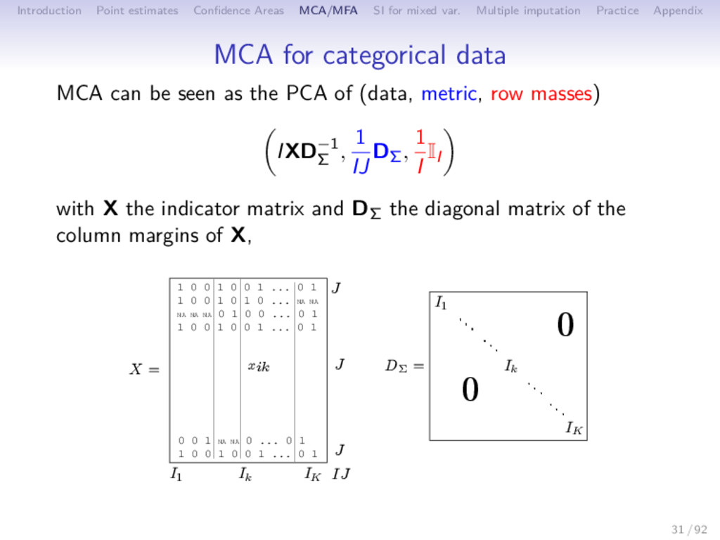
Multiple imputation Practice Appendix MCA for categorical data MCA can be seen as the PCA of (data, metric, row masses) IXD−1 Σ , 1 IJ DΣ, 1 I II with X the indicator matrix and DΣ the diagonal matrix of the column margins of X, xik I1 Ik IK J J J IJ X = DΣ = I1 Ik IK . . . .. . . .. . . . . . . .. . . .. . . . . . . .. . . .. . . . . . . .. . . .. . . . 0 0 1 0 0 1 0 0 1 ... 0 1 1 0 0 1 0 1 0 ... NA NA NA NA NA 0 1 0 0 ... 0 1 1 0 0 1 0 0 1 ... 0 1 0 0 1 NA NA 0 ... 0 1 1 0 0 1 0 0 1 ... 0 1 31 / 92
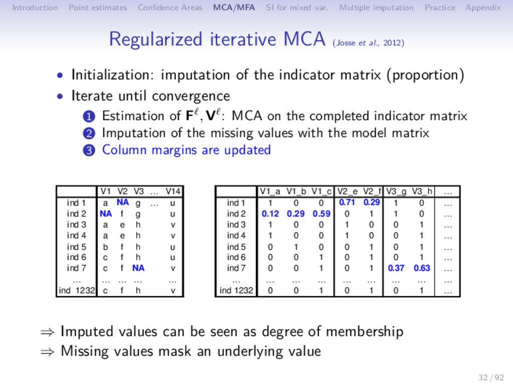
Multiple imputation Practice Appendix Regularized iterative MCA (Josse et al., 2012) • Initialization: imputation of the indicator matrix (proportion) • Iterate until convergence 1 Estimation of F , V : MCA on the completed indicator matrix 2 Imputation of the missing values with the model matrix 3 Column margins are updated V1 V2 V3 … V14 V1_a V1_b V1_c V2_e V2_f V3_g V3_h … ind 1 a NA g … u ind 1 1 0 0 0.71 0.29 1 0 … ind 2 NA f g u ind 2 0.12 0.29 0.59 0 1 1 0 … ind 3 a e h v ind 3 1 0 0 1 0 0 1 … ind 4 a e h v ind 4 1 0 0 1 0 0 1 … ind 5 b f h u ind 5 0 1 0 0 1 0 1 … ind 6 c f h u ind 6 0 0 1 0 1 0 1 … ind 7 c f NA v ind 7 0 0 1 0 1 0.37 0.63 … … … … … … … … … … … … … … … ind 1232 c f h v ind 1232 0 0 1 0 1 0 1 … ⇒ Imputed values can be seen as degree of membership ⇒ Missing values mask an underlying value 32 / 92
Multiple imputation Practice Appendix Multi-blocks data set • Biology: 10 samples without expression data • Sensory analysis: each judge can’t evaluate more than a certain number of products (saturation) Planned missing products judge, experimental design: BIB ⇒ Missing rows per subtable ⇒ Regularized iterative MFA (Husson & Josse, 2013) 34 / 92
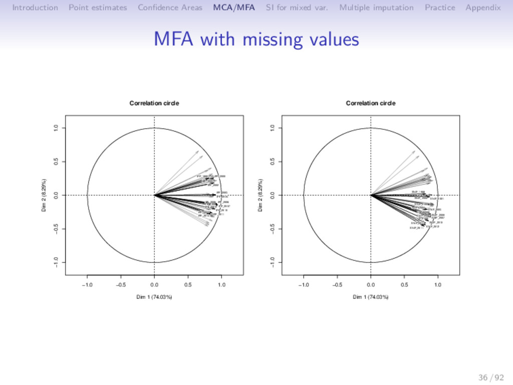
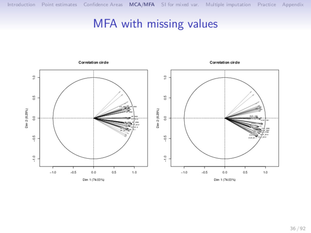
Multiple imputation Practice Appendix Journal impact factors journalmetrics.com provides 27000 journals/ 15 years of metrics. 443 journals (Computer Science, Statistics, Probability and Mathematics). 45 metrics, some may be NA, 15 years by 3 types of measures: • IPP - Impact Per Publication (like the ISI impact factor but for 3 (rather than 2) years. • SNIP - Source Normalized Impact Per Paper: Tries to weight by the number of citations per subject field to adjust for different citation cultures. • SJR - SCImago Journal Rank: Tries to capture average prestige per publication. 35 / 92
Multiple imputation Practice Appendix MFA with missing values -5 0 5 10 15 20 -4 -2 0 2 4 6 Journals Dim 1 (74.03%) Dim 2 (8.29%) ACM Transactions on Autonomous and Adaptive Systems ACM Transactions on Mathematical Software ACM Transactions on Programming Languages and Systems ACM Transactions on Software Engineering and Methodology Ad Hoc Networks Advances in Engineering Software (1978) Annals of Applied Probability Annals of Probability Annals of Statistics Bioinformatics Biometrics Biometrika Biostatistics Computer Vision and Image Understanding Finance and Stochastics IBM Systems Journal IEEE Micro IEEE Network IEEE Pervasive Computing IEEE Transactions on Affective Computing IEEE Transactions on Evolutionary Computation IEEE Transactions on Image Processing IEEE Transactions on Medical Imaging IEEE Transactions on Mobile Computing IEEE Transactions on Neural Networks IEEE Transactions on Pattern Analysis and Machine Intelligence IEEE Transactions on Software Engineering IEEE Transactions on Systems, Man and Cybernetics Part B: Cybernetics IEEE Transactions on Visualization and Computer Graphics IEEE/ACM Transactions on Networking Information Systems International Journal of Computer Vision International Journal of Robotics Research Journal of Business Journal of Business and Economic Statistics Journal of Cryptology Journal of Informetrics Journal of Machine Learning Research Journal of the ACM Journal of the American Society for Information Science and Technology Journal of the American Statistical Association Journal of the Royal Statistical Society. Series B: Statistical Methodology Machine Learning Mathematical Programming, Series B Multivariate Behavioral Research New Zealand Statistician Pattern Recognition Physical Review E - Statistical, Nonlinear, and Soft Matter Physics Probability Surveys Probability Theory and Related Fields Journal of Computational and Graphical Statistics R Journal Annals of Applied Statistics Journal of Statistical Software 36 / 92
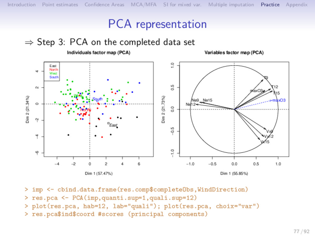
Multiple imputation Practice Appendix After performing principal component methods despite missing entries (getting the graphical outputs and the principal component and axes), we use these methods as tools of single and multiple imputation and compare them to the state of the art methods. PC methods are powerful to impute, since they use similarities between rows, relationship between columns and require a small number of parameters (dimensionality reduction) With single imputation, the aim to complete a dataset as best as possible (prediction). With multiple imputation the aim is to perform other statistical methods after and to estimate parameters and their variability taking into account the missing values uncertainty. 37 / 92
Multiple imputation Practice Appendix Outline 1 Introduction 2 Point estimates of the PCA axes and components 3 Uncertainty 4 MCA/MFA 5 Single imputation for mixed variables 6 Multiple imputation 7 Practice 8 Appendix 38 / 92
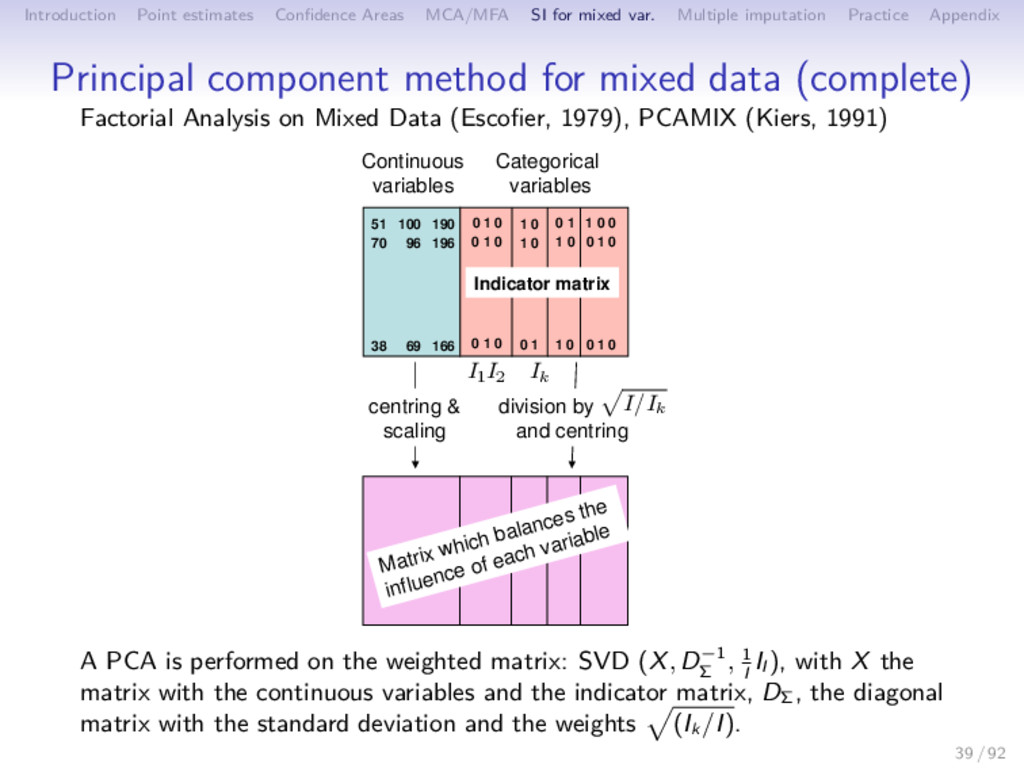
Multiple imputation Practice Appendix Principal component method for mixed data (complete) Factorial Analysis on Mixed Data (Escofier, 1979), PCAMIX (Kiers, 1991) Categorical variables Continuous variables 0 1 0 1 0 centring & scaling I1 I2 Ik division by and centring I/Ik 0 1 0 1 0 0 1 0 0 1 51 100 190 70 96 196 38 69 166 0 1 1 0 1 0 1 0 0 0 1 0 0 1 0 Indicator matrix Matrix which balances the influence of each variable A PCA is performed on the weighted matrix: SVD (X, D−1 Σ , 1 I II ), with X the matrix with the continuous variables and the indicator matrix, DΣ , the diagonal matrix with the standard deviation and the weights (Ik /I). 39 / 92
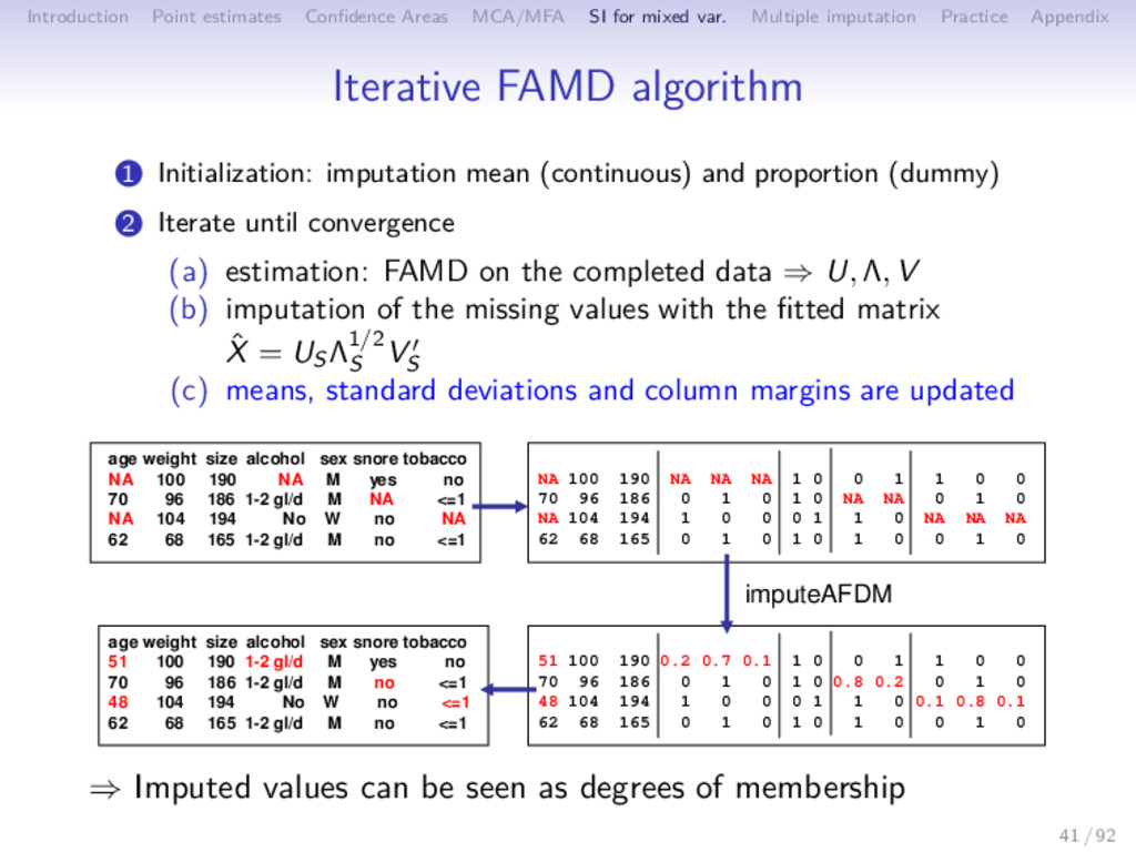
Multiple imputation Practice Appendix Iterative FAMD algorithm 1 Initialization: imputation mean (continuous) and proportion (dummy) 2 Iterate until convergence (a) estimation: FAMD on the completed data ⇒ U, Λ, V (b) imputation of the missing values with the fitted matrix ˆ X = US Λ1/2 S VS (c) means, standard deviations and column margins are updated age weight size alcohol sex snore tobacco NA 100 190 NA M yes no 70 96 186 1-2 gl/d M NA <=1 NA 104 194 No W no NA 62 68 165 1-2 gl/d M no <=1 age weight size alcohol sex snore tobacco 51 100 190 1-2 gl/d M yes no 70 96 186 1-2 gl/d M no <=1 48 104 194 No W no <=1 62 68 165 1-2 gl/d M no <=1 51 100 190 0.2 0.7 0.1 1 0 0 1 1 0 0 70 96 186 0 1 0 1 0 0.8 0.2 0 1 0 48 104 194 1 0 0 0 1 1 0 0.1 0.8 0.1 62 68 165 0 1 0 1 0 1 0 0 1 0 NA 100 190 NA NA NA 1 0 0 1 1 0 0 70 96 186 0 1 0 1 0 NA NA 0 1 0 NA 104 194 1 0 0 0 1 1 0 NA NA NA 62 68 165 0 1 0 1 0 1 0 0 1 0 imputeAFDM ⇒ Imputed values can be seen as degrees of membership 41 / 92
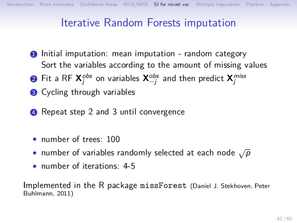
Multiple imputation Practice Appendix Iterative Random Forests imputation 1 Initial imputation: mean imputation - random category Sort the variables according to the amount of missing values 2 Fit a RF Xobs j on variables Xobs −j and then predict Xmiss j 3 Cycling through variables 4 Repeat step 2 and 3 until convergence • number of trees: 100 • number of variables randomly selected at each node √ p • number of iterations: 4-5 Implemented in the R package missForest (Daniel J. Stekhoven, Peter Buhlmann, 2011) 42 / 92
Multiple imputation Practice Appendix Simulation study Several data sets • Relationships between variables • Number of categories • percentage of missing values (10%,20%,30%) Criteria: • for continuous data: RMSE • for categorical data: proportion of falsely classified entries 43 / 92
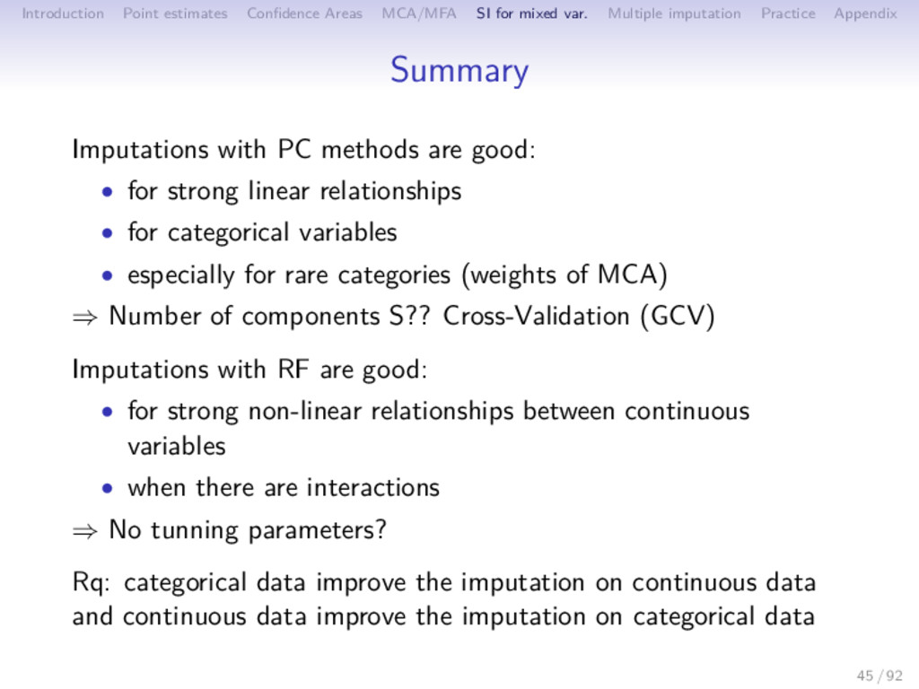
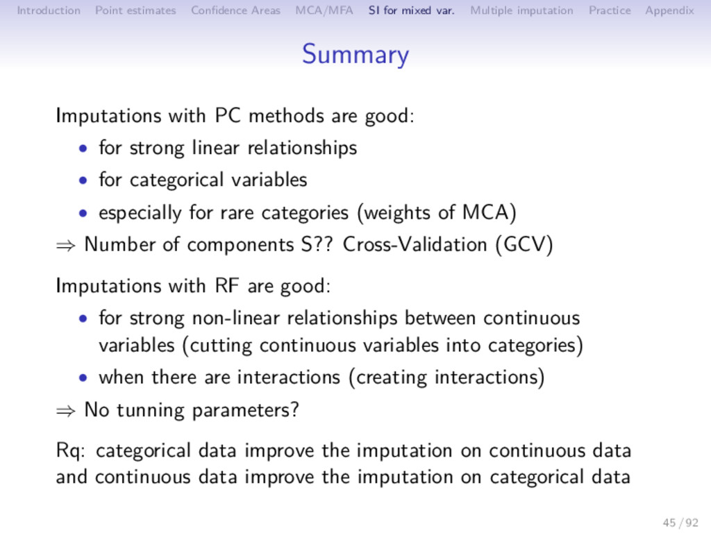
Multiple imputation Practice Appendix Summary Imputations with PC methods are good: • for strong linear relationships • for categorical variables • especially for rare categories (weights of MCA) ⇒ Number of components S?? Cross-Validation (GCV) Imputations with RF are good: • for strong non-linear relationships between continuous variables • when there are interactions ⇒ No tunning parameters? Rq: categorical data improve the imputation on continuous data and continuous data improve the imputation on categorical data 45 / 92
Multiple imputation Practice Appendix Summary Imputations with PC methods are good: • for strong linear relationships • for categorical variables • especially for rare categories (weights of MCA) ⇒ Number of components S?? Cross-Validation (GCV) Imputations with RF are good: • for strong non-linear relationships between continuous variables (cutting continuous variables into categories) • when there are interactions (creating interactions) ⇒ No tunning parameters? Rq: categorical data improve the imputation on continuous data and continuous data improve the imputation on categorical data 45 / 92
Multiple imputation Practice Appendix Outline 1 Introduction 2 Point estimates of the PCA axes and components 3 Uncertainty 4 MCA/MFA 5 Single imputation for mixed variables 6 Multiple imputation 7 Practice 8 Appendix 46 / 92
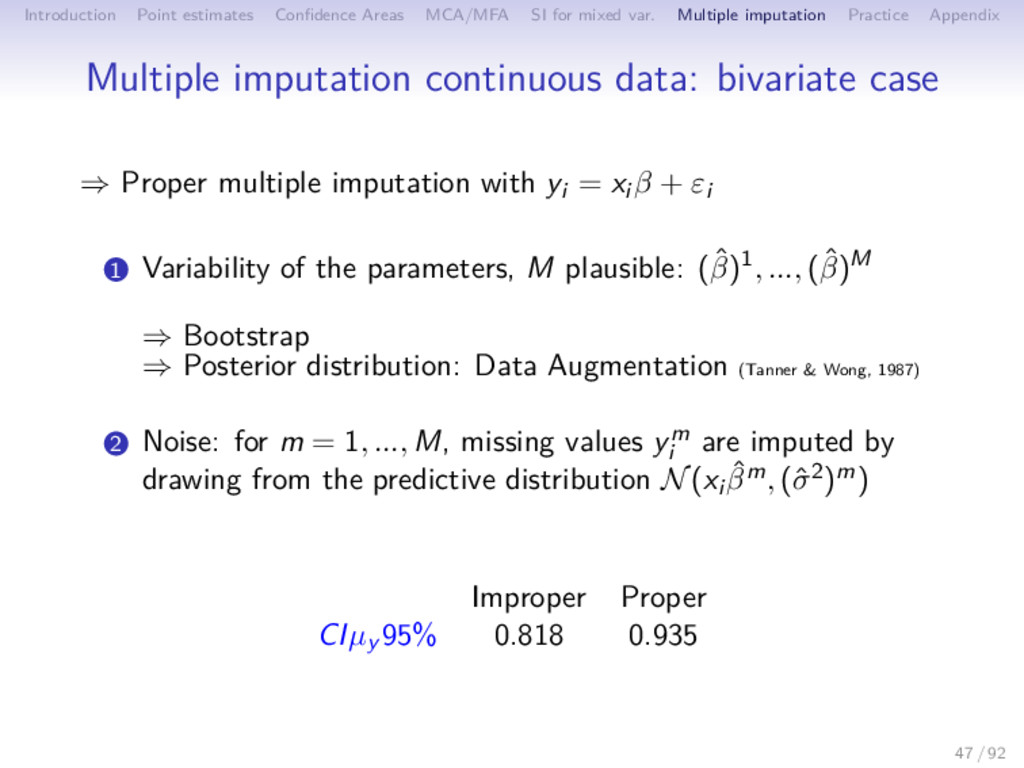
Multiple imputation Practice Appendix Multiple imputation continuous data: bivariate case ⇒ Proper multiple imputation with yi = xi β + εi 1 Variability of the parameters, M plausible: (ˆ β)1, ..., (ˆ β)M ⇒ Bootstrap ⇒ Posterior distribution: Data Augmentation (Tanner & Wong, 1987) 2 Noise: for m = 1, ..., M, missing values ym i are imputed by drawing from the predictive distribution N(xi ˆ βm, (ˆ σ2)m) Improper Proper CIµy 95% 0.818 0.935 47 / 92
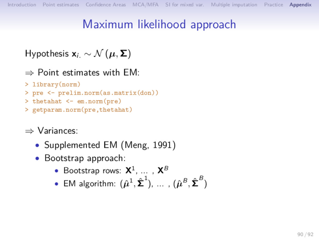
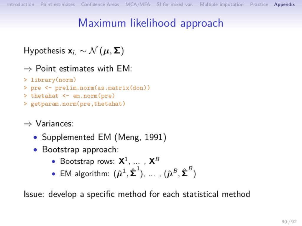
Multiple imputation Practice Appendix Joint modeling ⇒ Hypothesis xi. ∼ N (µ, Σ) Algorithm Expectation Maximization Bootstrap: 1 Bootstrap rows: X1, ... , XM EM algorithm: (ˆ µ1, ˆ Σ1), ... , (ˆ µM, ˆ ΣM) 2 Imputation: xm ij drawn from N ˆ µm, ˆ Σm Easy to parallelized. Implemented in Amelia (website) Amelia Earhart James Honaker Gary King Matt Blackwell 48 / 92
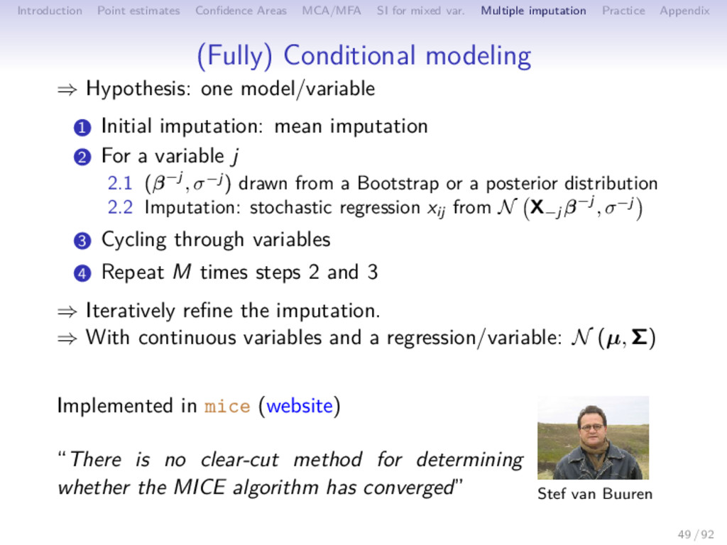
Multiple imputation Practice Appendix (Fully) Conditional modeling ⇒ Hypothesis: one model/variable 1 Initial imputation: mean imputation 2 For a variable j 2.1 (β−j , σ−j ) drawn from a Bootstrap or a posterior distribution 2.2 Imputation: stochastic regression xij from N X−j β−j , σ−j 3 Cycling through variables 4 Repeat M times steps 2 and 3 ⇒ Iteratively refine the imputation. Implemented in mice (website) “There is no clear-cut method for determining whether the MICE algorithm has converged” Stef van Buuren 49 / 92
Multiple imputation Practice Appendix (Fully) Conditional modeling ⇒ Hypothesis: one model/variable 1 Initial imputation: mean imputation 2 For a variable j 2.1 (β−j , σ−j ) drawn from a Bootstrap or a posterior distribution 2.2 Imputation: stochastic regression xij from N X−j β−j , σ−j 3 Cycling through variables 4 Repeat M times steps 2 and 3 ⇒ Iteratively refine the imputation. ⇒ With continuous variables and a regression/variable: N (µ, Σ) Implemented in mice (website) “There is no clear-cut method for determining whether the MICE algorithm has converged” Stef van Buuren 49 / 92
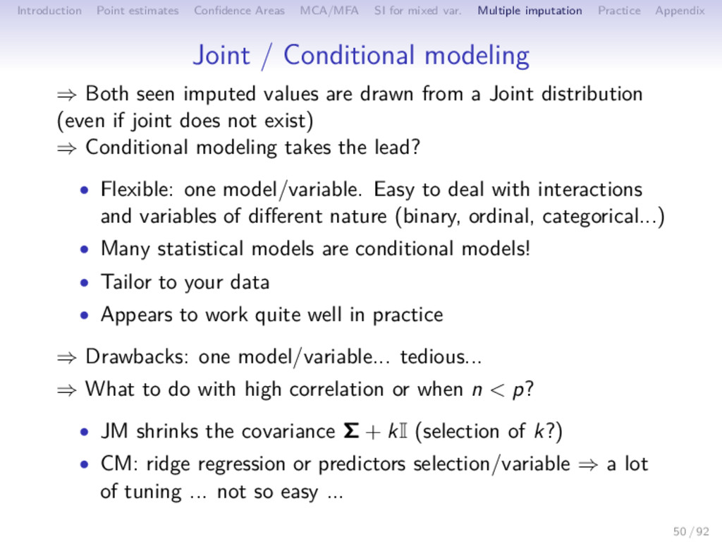
Multiple imputation Practice Appendix Joint / Conditional modeling ⇒ Both seen imputed values are drawn from a Joint distribution (even if joint does not exist) ⇒ Conditional modeling takes the lead? • Flexible: one model/variable. Easy to deal with interactions and variables of different nature (binary, ordinal, categorical...) • Many statistical models are conditional models! • Tailor to your data • Appears to work quite well in practice ⇒ Drawbacks: one model/variable... tedious... 50 / 92
Multiple imputation Practice Appendix Joint / Conditional modeling ⇒ Both seen imputed values are drawn from a Joint distribution (even if joint does not exist) ⇒ Conditional modeling takes the lead? • Flexible: one model/variable. Easy to deal with interactions and variables of different nature (binary, ordinal, categorical...) • Many statistical models are conditional models! • Tailor to your data • Appears to work quite well in practice ⇒ Drawbacks: one model/variable... tedious... ⇒ What to do with high correlation or when n < p? • JM shrinks the covariance Σ + kI (selection of k?) • CM: ridge regression or predictors selection/variable ⇒ a lot of tuning ... not so easy ... 50 / 92
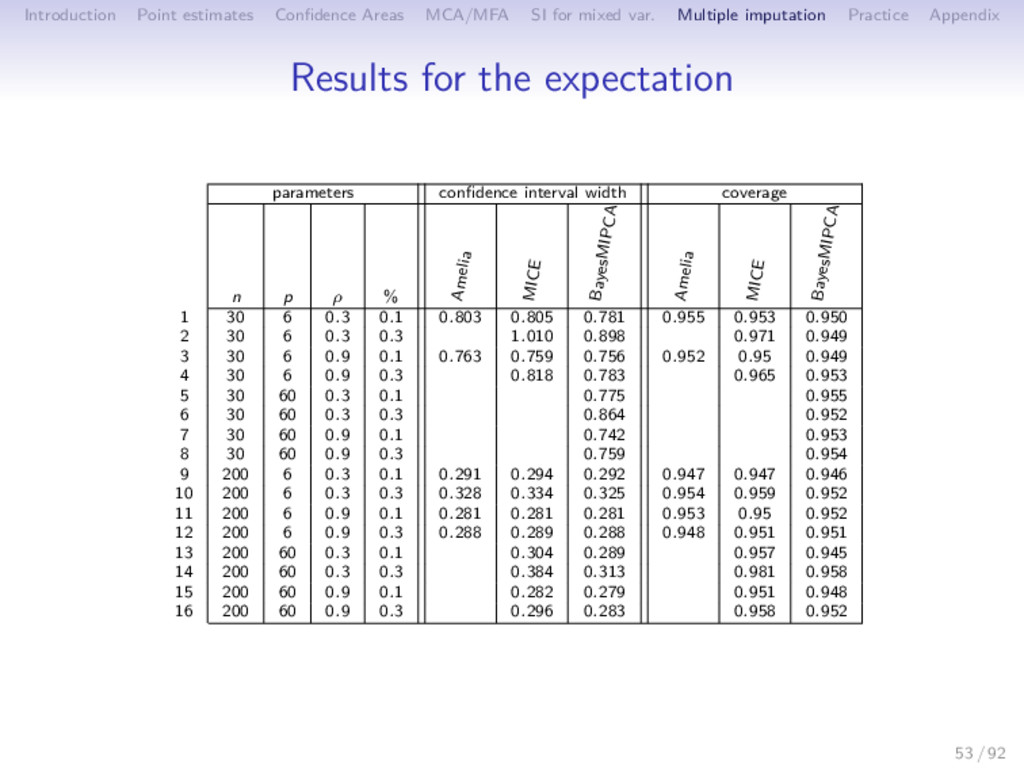
Multiple imputation Practice Appendix Simulations • 1000 simulations • data set drawn from Np (µ, Σ) with a two-block structure, varying n (30 or 200), p (6 or 60) and ρ (0.3 or 0.9) 0 0 0 0 0 0 0 0 0.8 0.8 0.8 0.8 0.8 0.8 0.8 0.8 0.8 0.8 0.8 0.8 0.8 0.8 0.8 0.8 • 10% or 30% of missing values using a MCAR mechanism • multiple imputation using M = 20 imputed data • Quantities of interest: θ1 = E [Y ] , θ2 = β1, θ3 = ρ • Criteria • bias • CI width, coverage 52 / 92
Multiple imputation Practice Appendix Joint, conditional and PCA ⇒ Good estimates of the parameters and their variance from an incomplete data (coverage close to 0.95) The variability due to missing values is well taken into account Amelia & mice have difficulties with large correlations or n < p missMDA does not but requires a tuning parameter: number of dim. Amelia & missMDA are based on linear relationships mice is more flexible (one model per variable) MI based on PCA works in a large range of configuration, n < p, n > p strong or weak relationships, low or high percentage of missing values 54 / 92
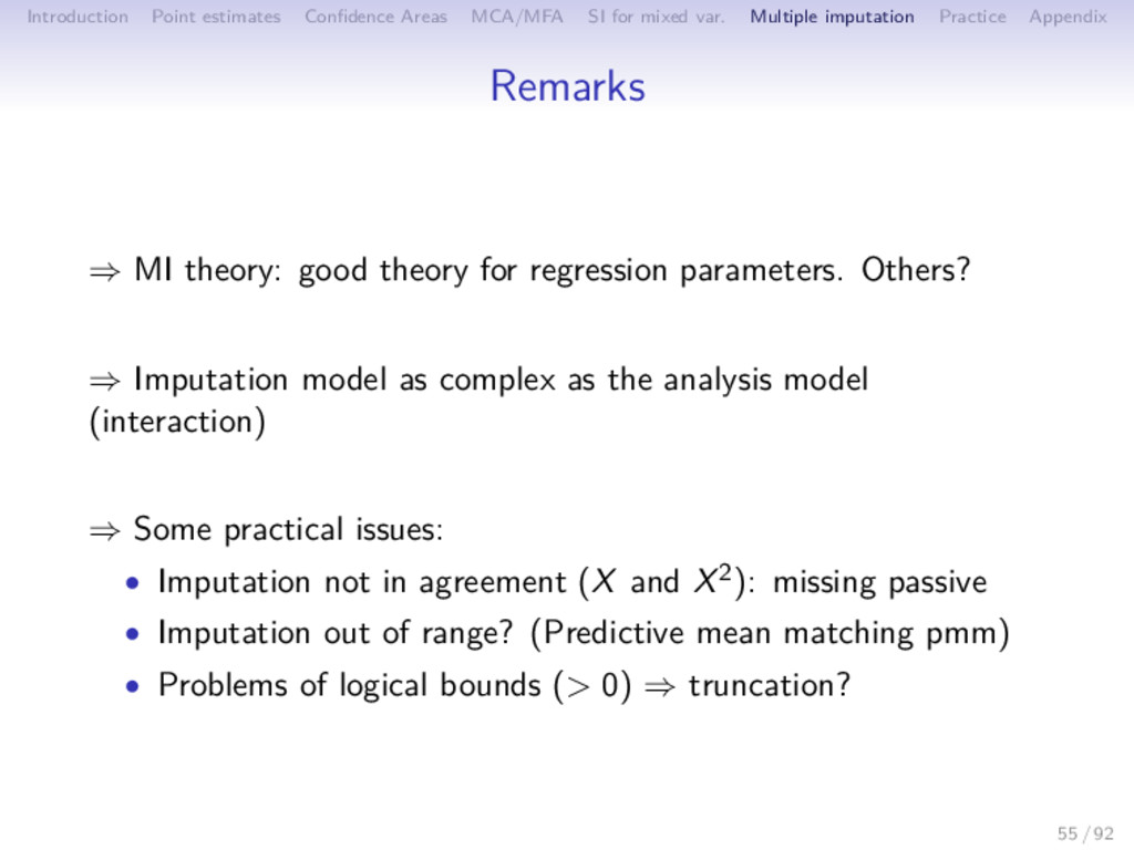
Multiple imputation Practice Appendix Remarks ⇒ MI theory: good theory for regression parameters. Others? ⇒ Imputation model as complex as the analysis model (interaction) 55 / 92
Multiple imputation Practice Appendix Remarks ⇒ MI theory: good theory for regression parameters. Others? ⇒ Imputation model as complex as the analysis model (interaction) ⇒ Some practical issues: • Imputation not in agreement (X and X2): missing passive • Imputation out of range? (Predictive mean matching pmm) • Problems of logical bounds (> 0) ⇒ truncation? 55 / 92
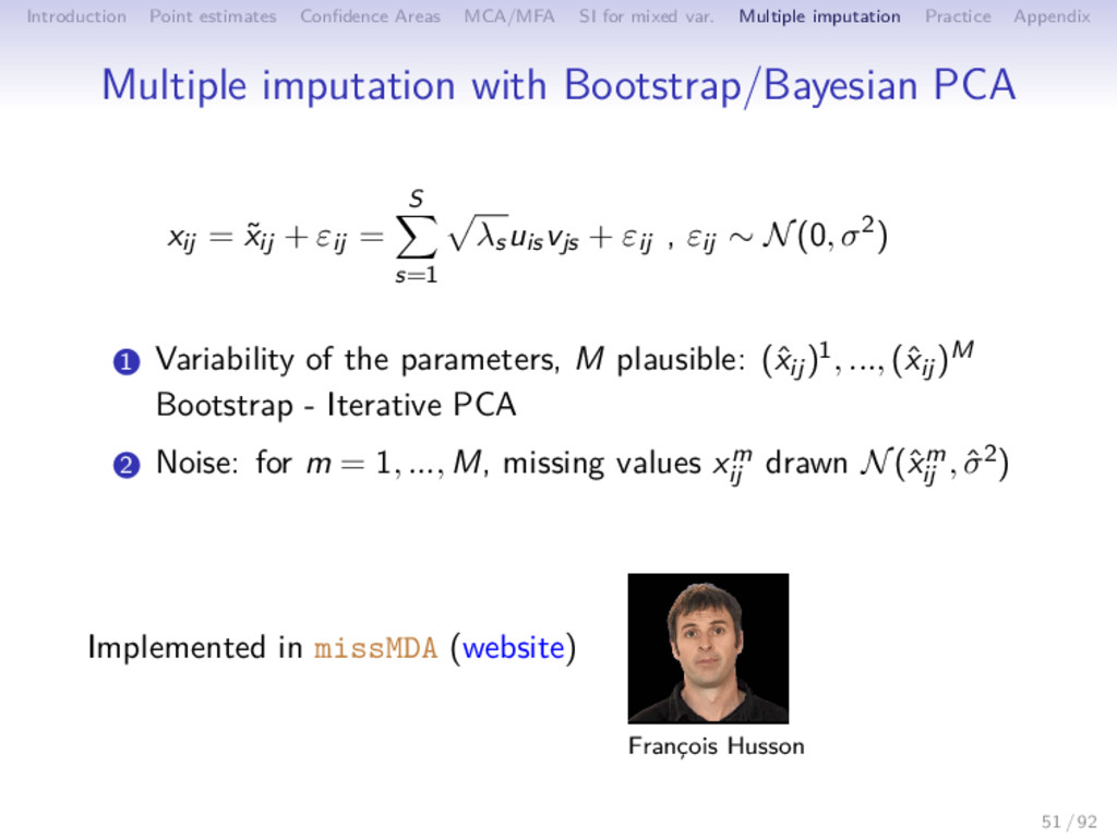
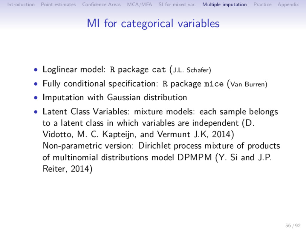
Multiple imputation Practice Appendix MI for categorical variables • Loglinear model: R package cat (J.L. Schafer) • Fully conditional specification: R package mice (Van Burren) • Imputation with Gaussian distribution • Latent Class Variables: mixture models: each sample belongs to a latent class in which variables are independent (D. Vidotto, M. C. Kapteijn, and Vermunt J.K, 2014) Non-parametric version: Dirichlet process mixture of products of multinomial distributions model DPMPM (Y. Si and J.P. Reiter, 2014) 56 / 92
Multiple imputation Practice Appendix Multiple imputation for categorical data using MCA A set of parameters: UI×S , Λ1/2 S×S , VJ×S 1 , . . . , UI×S , Λ1/2 S×S , VJ×S M obtained using a non-parametric Bootstrap approach: 1 Generate M bootstrap replicates 2 Estimate the parameters on each incomplete replicate 3 Add uncertainty on the prediction 57 / 92
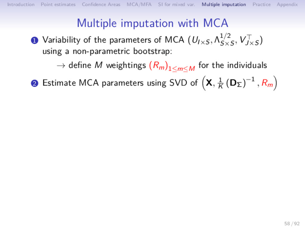
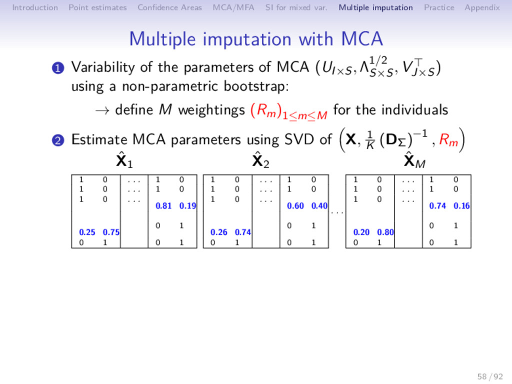
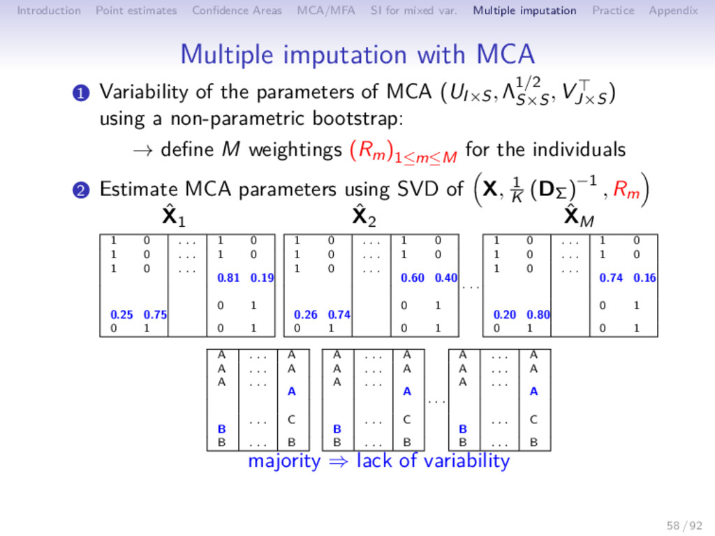
Multiple imputation Practice Appendix Multiple imputation with MCA 1 Variability of the parameters of MCA (UI×S, Λ1/2 S×S , VJ×S ) using a non-parametric bootstrap: → define M weightings (Rm)1≤m≤M for the individuals 58 / 92
Multiple imputation Practice Appendix Multiple imputation with MCA 1 Variability of the parameters of MCA (UI×S, Λ1/2 S×S , VJ×S ) using a non-parametric bootstrap: → define M weightings (Rm)1≤m≤M for the individuals 2 Estimate MCA parameters using SVD of X, 1 K (DΣ)−1 , Rm 58 / 92
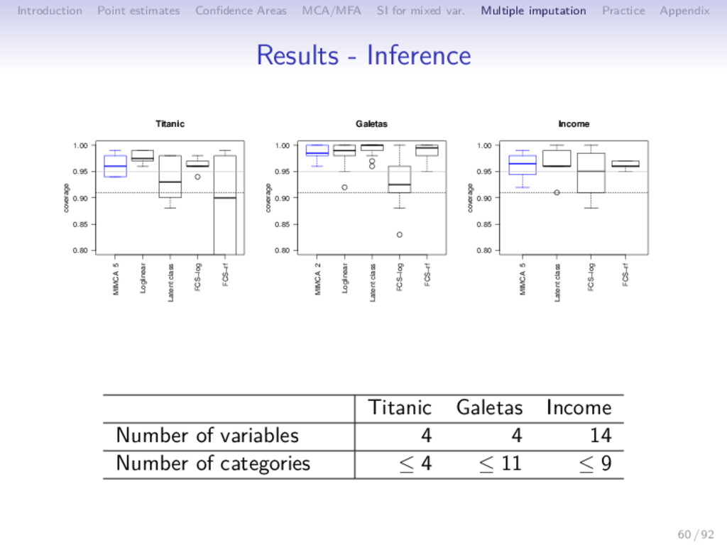
Multiple imputation Practice Appendix Simulations • Quantities of interest: θ = parameters of a logistic model • 200 simulations from real data sets • the real data set is considered as a population • drawn one sample from the data set • generate 20% of missing values • multiple imputation using M = 5 imputed data • Criteria • bias • CI width, coverage 59 / 92
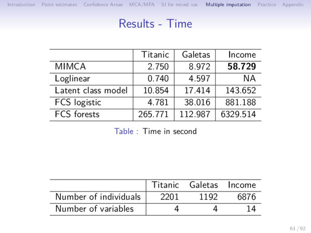
Multiple imputation Practice Appendix Results - Time Titanic Galetas Income MIMCA 2.750 8.972 58.729 Loglinear 0.740 4.597 NA Latent class model 10.854 17.414 143.652 FCS logistic 4.781 38.016 881.188 FCS forests 265.771 112.987 6329.514 Table : Time in second Titanic Galetas Income Number of individuals 2201 1192 6876 Number of variables 4 4 14 61 / 92
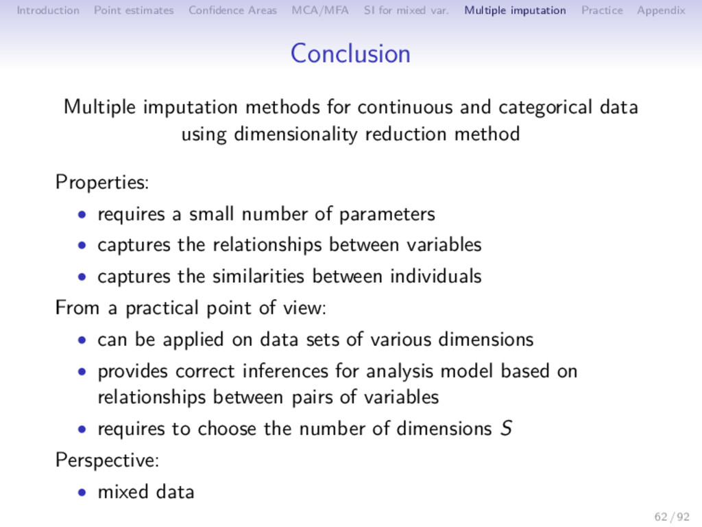
Multiple imputation Practice Appendix Conclusion Multiple imputation methods for continuous and categorical data using dimensionality reduction method Properties: • requires a small number of parameters • captures the relationships between variables • captures the similarities between individuals From a practical point of view: • can be applied on data sets of various dimensions • provides correct inferences for analysis model based on relationships between pairs of variables • requires to choose the number of dimensions S Perspective: • mixed data 62 / 92
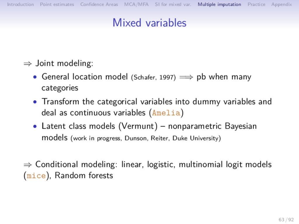
Multiple imputation Practice Appendix Mixed variables ⇒ Joint modeling: • General location model (Schafer, 1997) =⇒ pb when many categories • Transform the categorical variables into dummy variables and deal as continuous variables (Amelia) • Latent class models (Vermunt) – nonparametric Bayesian models (work in progress, Dunson, Reiter, Duke University) ⇒ Conditional modeling: linear, logistic, multinomial logit models (mice), Random forests 63 / 92
Multiple imputation Practice Appendix To conclude Take home message: • “The idea of imputation is both seductive and dangerous. It is seductive because it can lull the user into the pleasurable state of believing that the data are complete after all, and it is dangerous because it lumps together situations where the problem is sufficiently minor that it can be legitimately handled in this way and situations where standard estimators applied to the real and imputed data have substantial biases.” (Dempster and Rubin, 1983) • Advanced methods are available to estimate parameters and their variance (taking into account the variability due to missing values) • Multiple imputation is an appealing method .... but ... how can we do with big data? • Still an active area of research 64 / 92
Multiple imputation Practice Appendix Ressources ⇒ Softwares: • van Buuren webpage: http://www.stefvanbuuren.nl/mi/Software.html • R task View: Official Statistics & Survey Methodology ⇒ Recent Books: • van Buuren (2012). Flexible Imputation of Missing Data. Chapman & Hall/CRC • Carpenter & Kenward (2013). Multiple Imputation and its Application. Wiley • G. Molenberghs, G. Fitzmaurice, M.G. Kenward, A. Tsiatis & G. Verbeke (nov 2014). Handbook of Missing Data. Chapman & Hall/CRC ⇒ Little & Rubin (2002). Statistical Analysis with missing data - Schafer (1997) Analysis of incomplete multivariate data ⇒ J.L. Schafer & J.W. Graham, 2002. Missing Data: Our View of the State of the Art. Psychological Methods, 7 147-177 ⇒ B. Efron. 1989. Missing data, Imputation and the Bootstrap. Journal of the American Statistical Association, 426 463-475 65 / 92
Multiple imputation Practice Appendix Contributors on the topic of multiple imputation • J. Honaker - G. King - M. Blackwell (Harvard): Amelia • S. van Buuren (Utrecht): mice • F. Husson - J. Josse (Rennes): missMDA • A. Gelman - J. Hill - Y. Su (Colombia): mi • J. Reiter (Duke): NPBayesImpute Non-Parametric Bayesian Multiple Imputation for Categorical Data • J. Bartlett - J. Carpenter - M. Kenward (UCL): smcfcs Substantive model compatible FCS multiple imputation • H. Goldstein (Bristol) : realcom for multi-level data • J.K. Vermunt (Tilburg): poLCA latent class models • Shaun Seaman (Medical Research Council Biostatistics Unit, UK), Roderick Little (Michigan)... • Donald B Rubin (Harvard) 66 / 92
Multiple imputation Practice Appendix Outline 1 Introduction 2 Point estimates of the PCA axes and components 3 Uncertainty 4 MCA/MFA 5 Single imputation for mixed variables 6 Multiple imputation 7 Practice 8 Appendix 68 / 92
Multiple imputation Practice Appendix Outline 1 Introduction 2 Point estimates of the PCA axes and components 3 Uncertainty 4 MCA/MFA 5 Single imputation for mixed variables 6 Multiple imputation 7 Practice 8 Appendix 88 / 92
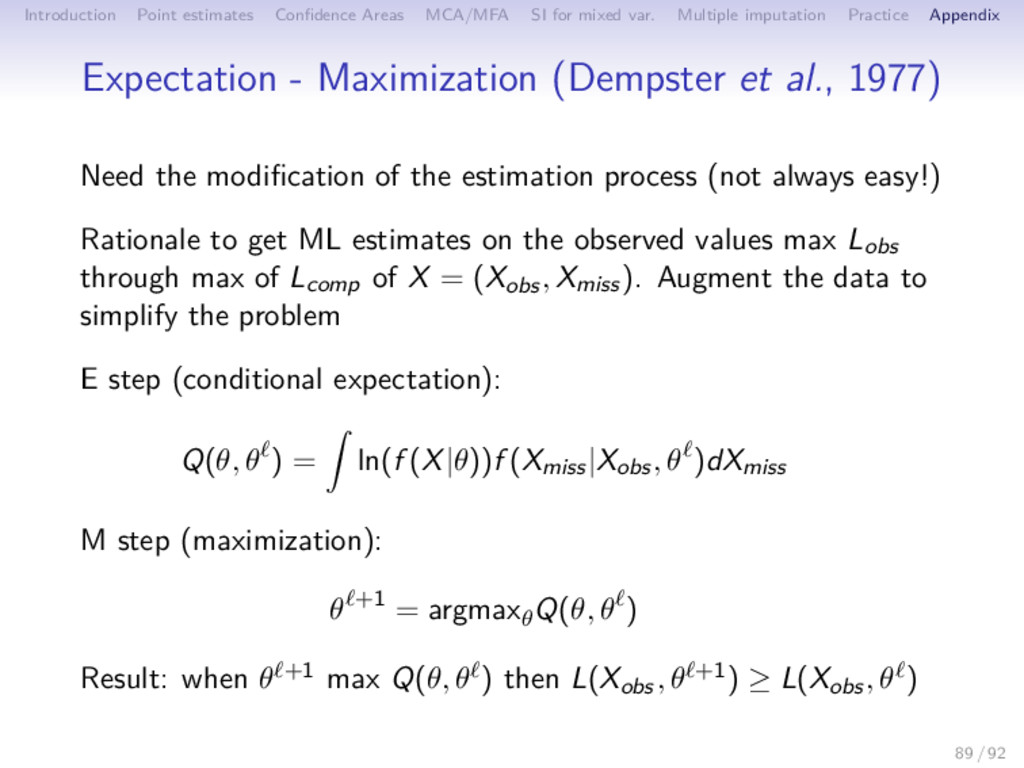
Multiple imputation Practice Appendix Expectation - Maximization (Dempster et al., 1977) Need the modification of the estimation process (not always easy!) Rationale to get ML estimates on the observed values max Lobs through max of Lcomp of X = (Xobs, Xmiss). Augment the data to simplify the problem E step (conditional expectation): Q(θ, θ ) = ln(f (X|θ))f (Xmiss|Xobs, θ )dXmiss M step (maximization): θ +1 = argmaxθ Q(θ, θ ) Result: when θ +1 max Q(θ, θ ) then L(Xobs, θ +1) ≥ L(Xobs, θ ) 89 / 92
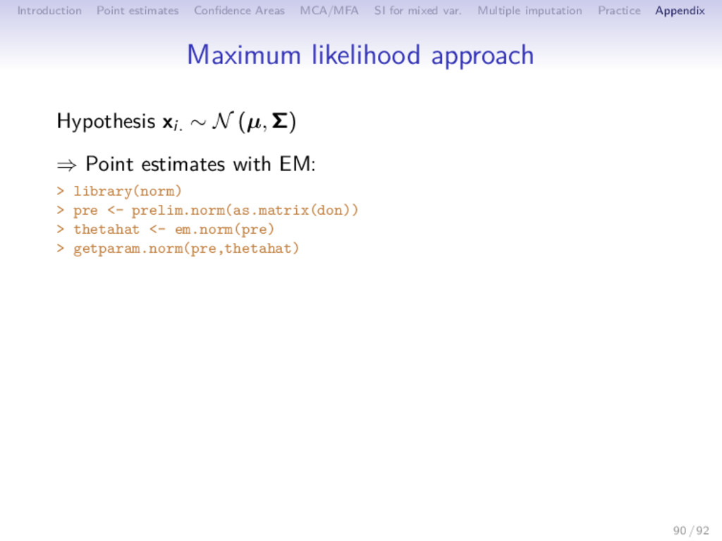
Multiple imputation Practice Appendix Maximum likelihood approach Hypothesis xi. ∼ N (µ, Σ) ⇒ Point estimates with EM: > library(norm) > pre <- prelim.norm(as.matrix(don)) > thetahat <- em.norm(pre) > getparam.norm(pre,thetahat) 90 / 92
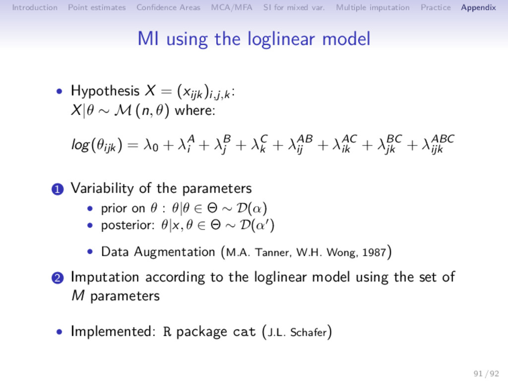
Multiple imputation Practice Appendix MI using the loglinear model • Hypothesis X = (xijk)i,j,k: X|θ ∼ M (n, θ) where: log(θijk) = λ0 + λA i + λB j + λC k + λAB ij + λAC ik + λBC jk + λABC ijk 1 Variability of the parameters • prior on θ : θ|θ ∈ Θ ∼ D(α) • posterior: θ|x, θ ∈ Θ ∼ D(α ) • Data Augmentation (M.A. Tanner, W.H. Wong, 1987) 2 Imputation according to the loglinear model using the set of M parameters • Implemented: R package cat (J.L. Schafer) 91 / 92
Multiple imputation Practice Appendix MI using a DPMPM model (Si and Reiter, 2013) • Hypothesis: P (X = (x1, . . . , xK ); θ) = L =1 θ K k=1 θ( ) xk 1 Variability of the parameters: • a hierarchic prior on θ: α ∼ G(.25, .25) ζ ∼ B(1, α) θ = ζ g< (1 − ζg ) for in 1, . . . , ∞ • posterior on θ: untractable → Gibbs sampler and Data Augmentation 2 Imputation according to the mixture model using the set of M parameters • Implemented: R package mi (Gelman et al.) 92 / 92