Multiple imputation for mixed data

defense of vincent audigier

Transcript

1. Introduction Single Imputation MI with PCA MI with MCA Conclusion References Multiple imputation with principal component methods Vincent Audigier Agrocampus Ouest, Rennes PhD defense, November 25, 2015 1 / 37
2. Introduction Single Imputation MI with PCA MI with MCA Conclusion References 1 Introduction 2 Single imputation based on principal component methods 3 Multiple imputation for continuous data with PCA 4 Multiple imputation for categorical data with MCA 5 Conclusion 2 / 37
3. Introduction Single Imputation MI with PCA MI with MCA Conclusion References Missing values NA NA NA NA NA NA . . . . . . . . . . . . . . . . . . . . . . . . NA NA NA • Aim: inference on a quantity θ from incomplete data → point estimate ˆ θ and associated variability T 3 / 37
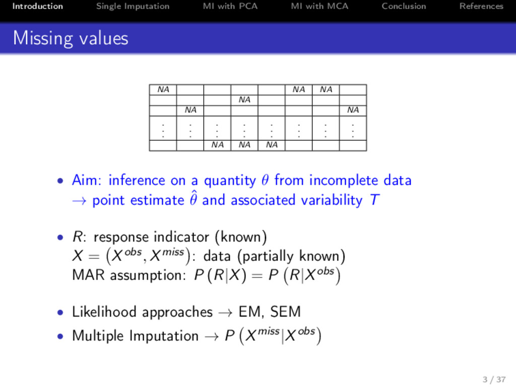
4. Introduction Single Imputation MI with PCA MI with MCA Conclusion References Missing values NA NA NA NA NA NA . . . . . . . . . . . . . . . . . . . . . . . . NA NA NA • Aim: inference on a quantity θ from incomplete data → point estimate ˆ θ and associated variability T • R: response indicator (known) X = Xobs, Xmiss : data (partially known) MAR assumption: P (R|X) = P R|Xobs • Likelihood approaches → EM, SEM • Multiple Imputation → P Xmiss|Xobs 3 / 37
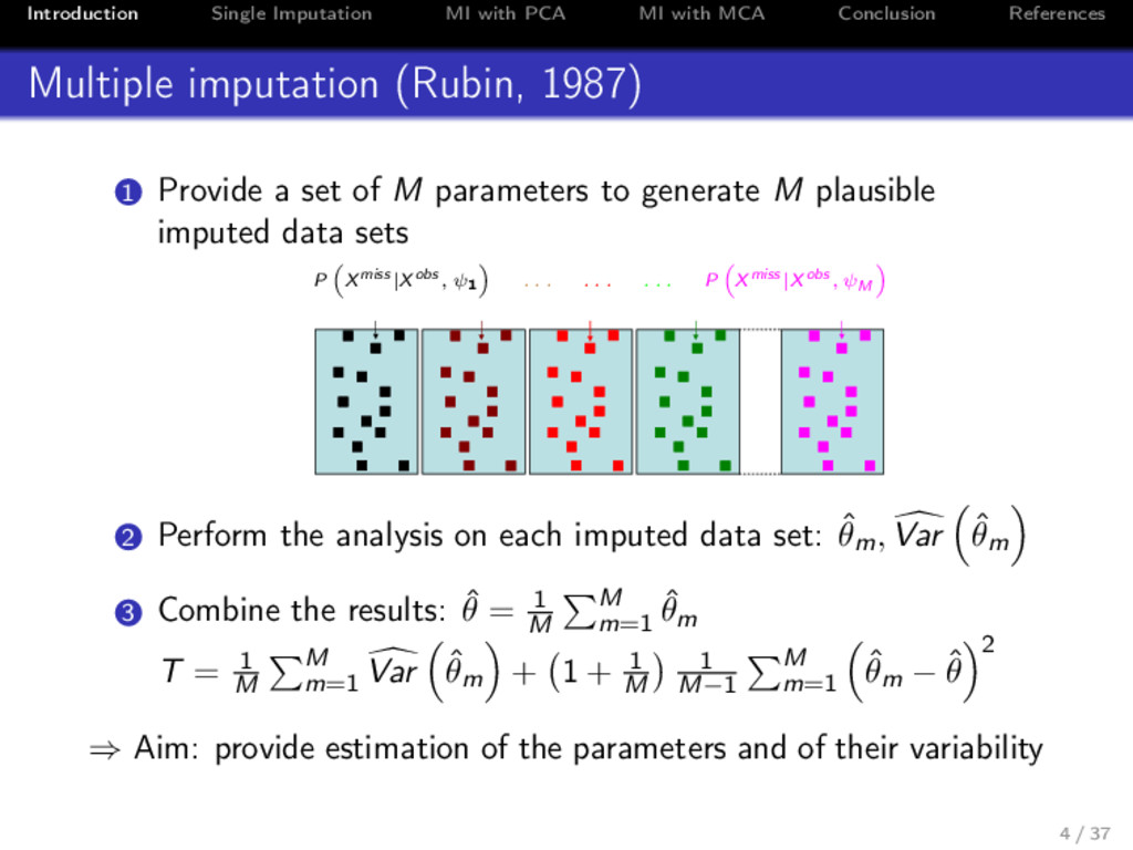
5. Introduction Single Imputation MI with PCA MI with MCA Conclusion References Multiple imputation (Rubin, 1987) 1 Provide a set of M parameters to generate M plausible imputed data sets P Xmiss |Xobs , ψ1 . . . . . . . . . P Xmiss |Xobs , ψM ( ˆ F ˆ u′)ij ( ˆ F ˆ u′)1 ij + ε1 ij ( ˆ F ˆ u′)2 ij + ε2 ij ( ˆ F ˆ u′)3 ij + ε3 ij ( ˆ F ˆ u′)B ij + εB ij 2 Perform the analysis on each imputed data set: ˆ θm, Var ˆ θm 3 Combine the results: ˆ θ = 1 M M m=1 ˆ θm T = 1 M M m=1 Var ˆ θm + 1 + 1 M 1 M−1 M m=1 ˆ θm − ˆ θ 2 ⇒ Aim: provide estimation of the parameters and of their variability 4 / 37
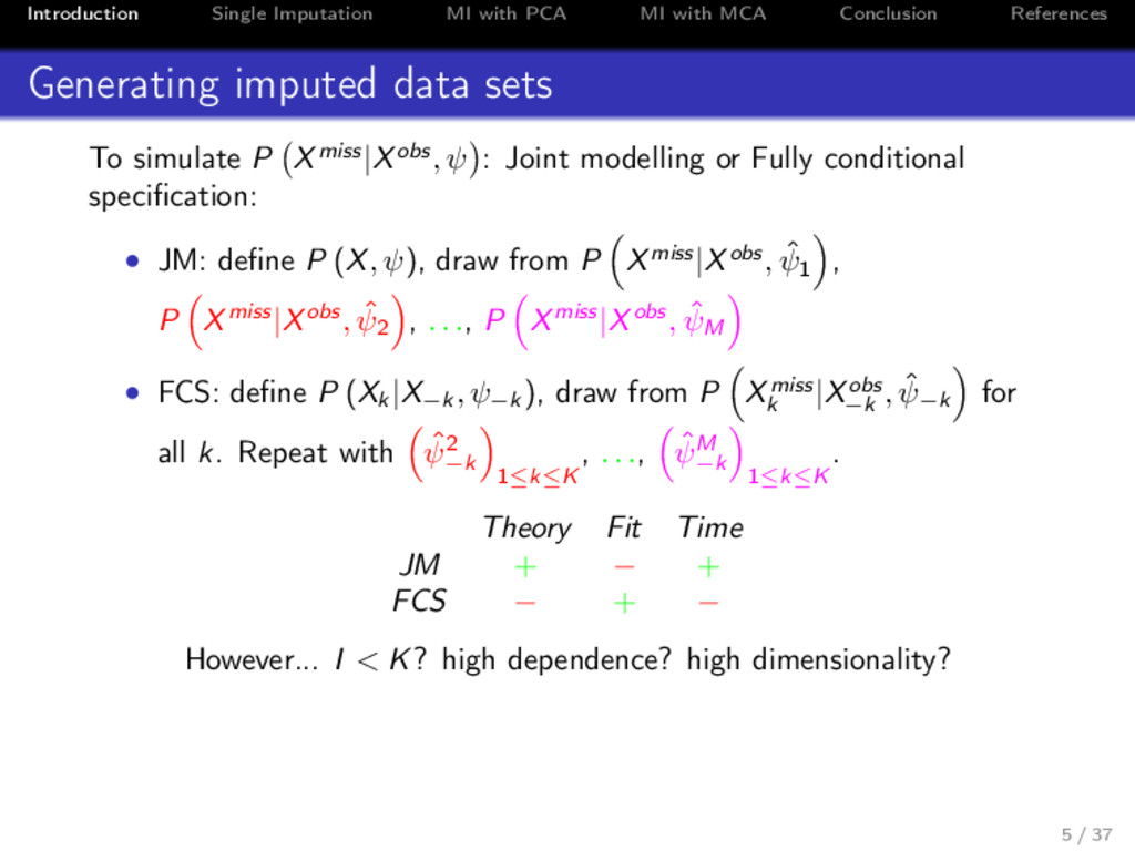
6. Introduction Single Imputation MI with PCA MI with MCA Conclusion References Generating imputed data sets To simulate P Xmiss|Xobs, ψ : Joint modelling or Fully conditional specification: • JM: define P (X, ψ), draw from P Xmiss|Xobs, ˆ ψ1 , P Xmiss|Xobs, ˆ ψ2 , . . ., P Xmiss|Xobs, ˆ ψM • FCS: define P (Xk |X−k , ψ−k ), draw from P Xmiss k |Xobs −k , ˆ ψ−k for all k. Repeat with ˆ ψ2 −k 1≤k≤K , . . ., ˆ ψM −k 1≤k≤K . Theory Fit Time JM + − + FCS − + − However... I < K? high dependence? high dimensionality? 5 / 37
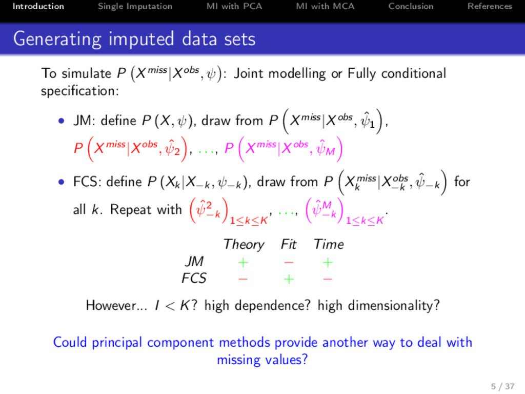
7. Introduction Single Imputation MI with PCA MI with MCA Conclusion References Generating imputed data sets To simulate P Xmiss|Xobs, ψ : Joint modelling or Fully conditional specification: • JM: define P (X, ψ), draw from P Xmiss|Xobs, ˆ ψ1 , P Xmiss|Xobs, ˆ ψ2 , . . ., P Xmiss|Xobs, ˆ ψM • FCS: define P (Xk |X−k , ψ−k ), draw from P Xmiss k |Xobs −k , ˆ ψ−k for all k. Repeat with ˆ ψ2 −k 1≤k≤K , . . ., ˆ ψM −k 1≤k≤K . Theory Fit Time JM + − + FCS − + − However... I < K? high dependence? high dimensionality? Could principal component methods provide another way to deal with missing values? 5 / 37
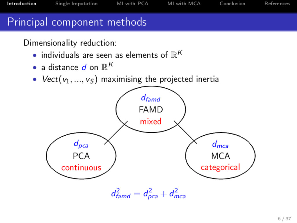
8. Introduction Single Imputation MI with PCA MI with MCA Conclusion References Principal component methods Dimensionality reduction: • individuals are seen as elements of RK • a distance d on RK • Vect(v1, ..., vS ) maximising the projected inertia dfamd FAMD mixed dpca PCA continuous dmca MCA categorical d2 famd = d2 pca + d2 mca 6 / 37
9. Introduction Single Imputation MI with PCA MI with MCA Conclusion References 1 Introduction 2 Single imputation based on principal component methods 3 Multiple imputation for continuous data with PCA 4 Multiple imputation for categorical data with MCA 5 Conclusion 7 / 37
10. Introduction Single Imputation MI with PCA MI with MCA Conclusion References How to perform FAMD? FAMD can be seen as the SVD of X with weights for • the continuous variables and categories: (DΣ)−1 • the individuals: 1 I 1I −→ SVD X, (DΣ)−1 , 1 I 1I 11.04 . . . 2.07 1 0 . . . 1 0 0 10.76 . . . 1.86 1 0 . . . 1 0 0 11.02 . . . 2.04 1 0 . . . 1 0 0 11.02 . . . 1.92 0 1 . . . 0 1 0 X = 11.06 2.01 0 1 0 0 1 10.95 1.67 0 1 0 1 0 σx1 . . . 0 σxk DΣ = Ik+1 0 . . . IK 8 / 37
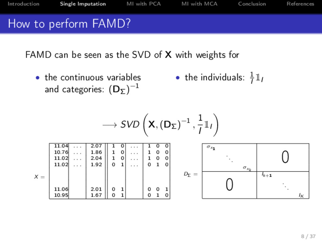
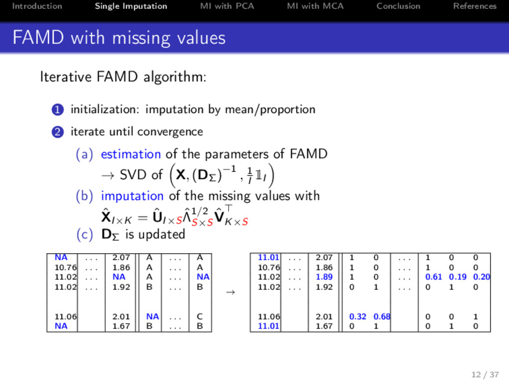
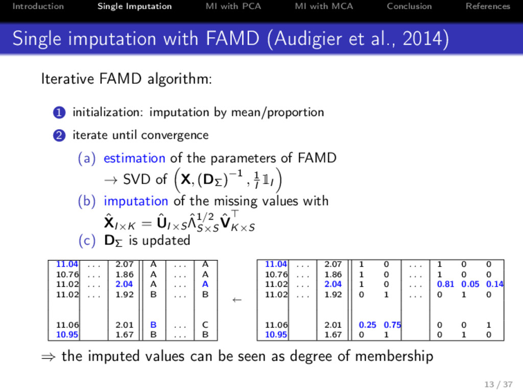
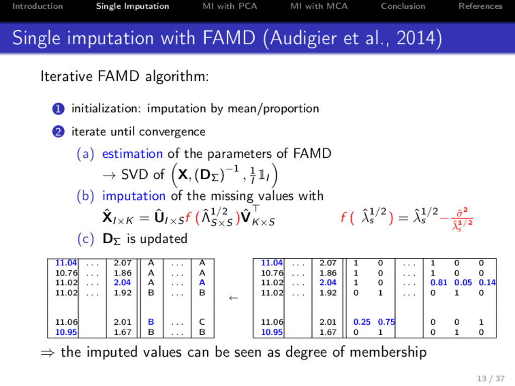
11. Introduction Single Imputation MI with PCA MI with MCA Conclusion References How to perform FAMD? SVD X, (DΣ)−1 , 1 I 1I −→ XI×K = UI×K Λ1/2 K×K VK×K with U 1 I 1I U = 1K V D−1 Σ V = 1K • principal components: ˆ FI×S = ˆ UI×S ˆ Λ1/2 S×S • loadings: ˆ VK×S • fitted matrix: ˆ XI×K = ˆ UI×S ˆ Λ1/2 S×S ˆ VK×S ˆ X − X 2 D−1 Σ ⊗1 I 1 = tr ˆ X − X D−1 Σ ˆ X − X 1 I 1I minimized under the constraint of rank S 9 / 37
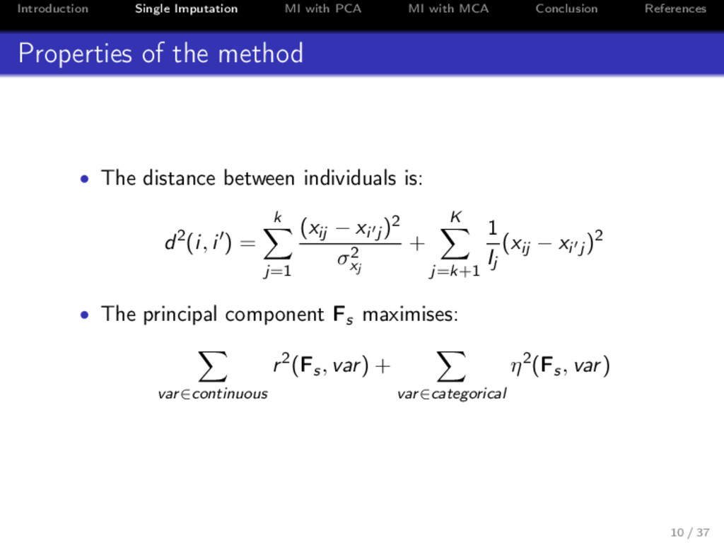
12. Introduction Single Imputation MI with PCA MI with MCA Conclusion References Properties of the method • The distance between individuals is: d2(i, i ) = k j=1 (xij − xi j )2 σ2 xj + K j=k+1 1 Ij (xij − xi j )2 • The principal component Fs maximises: var∈continuous r2(Fs, var) + var∈categorical η2(Fs, var) 10 / 37
13. Introduction Single Imputation MI with PCA MI with MCA Conclusion References FAMD with missing values ⇒ FAMD: least squares XI×K − UI×S Λ 1 2 S×S VK×S 2 ⇒ FAMD with missing values: weighted least squares WI×K ∗ (XI×K − UI×S Λ 1 2 S×S VK×S ) 2 with wij = 0 if xij is missing, wij = 1 otherwise Many algorithms developed for PCA such as NIPALS (Christoffersson, 1970) or iterative PCA (Kiers, 1997) 11 / 37
14. Introduction Single Imputation MI with PCA MI with MCA Conclusion References FAMD with missing values Iterative FAMD algorithm: 1 initialization: imputation by mean/proportion 2 iterate until convergence (a) estimation of the parameters of FAMD → SVD of X, (DΣ )−1 , 1 I 1I (b) imputation of the missing values with ˆ XI×K = ˆ UI×S ˆ Λ1/2 S×S ˆ VK×S (c) DΣ is updated NA . . . 2.07 A . . . A 10.76 . . . 1.86 A . . . A 11.02 . . . NA A . . . NA 11.02 . . . 1.92 B . . . B 11.06 2.01 NA . . . C NA 1.67 B . . . B → NA . . . 2.07 1 0 . . . 1 0 0 10.76 . . . 1.86 1 0 . . . 1 0 0 11.02 . . . NA 1 0 . . . NA NA NA 11.02 . . . 1.92 0 1 . . . 0 1 0 11.06 2.01 NA NA 0 0 1 NA 1.67 0 1 0 1 0 12 / 37
15. Introduction Single Imputation MI with PCA MI with MCA Conclusion References FAMD with missing values Iterative FAMD algorithm: 1 initialization: imputation by mean/proportion 2 iterate until convergence (a) estimation of the parameters of FAMD → SVD of X, (DΣ )−1 , 1 I 1I (b) imputation of the missing values with ˆ XI×K = ˆ UI×S ˆ Λ1/2 S×S ˆ VK×S (c) DΣ is updated NA . . . 2.07 A . . . A 10.76 . . . 1.86 A . . . A 11.02 . . . NA A . . . NA 11.02 . . . 1.92 B . . . B 11.06 2.01 NA . . . C NA 1.67 B . . . B → 11.01 . . . 2.07 1 0 . . . 1 0 0 10.76 . . . 1.86 1 0 . . . 1 0 0 11.02 . . . 1.89 1 0 . . . 0.61 0.19 0.20 11.02 . . . 1.92 0 1 . . . 0 1 0 11.06 2.01 0.32 0.68 0 0 1 11.01 1.67 0 1 0 1 0 12 / 37
16. Introduction Single Imputation MI with PCA MI with MCA Conclusion References FAMD with missing values Iterative FAMD algorithm: 1 initialization: imputation by mean/proportion 2 iterate until convergence (a) estimation of the parameters of FAMD → SVD of X, (DΣ )−1 , 1 I 1I (b) imputation of the missing values with ˆ XI×K = ˆ UI×S ˆ Λ1/2 S×S ˆ VK×S (c) DΣ is updated NA . . . 2.07 A . . . A 10.76 . . . 1.86 A . . . A 11.02 . . . NA A . . . NA 11.02 . . . 1.92 B . . . B 11.06 2.01 NA . . . C NA 1.67 B . . . B → 11.04 . . . 2.07 1 0 . . . 1 0 0 10.76 . . . 1.86 1 0 . . . 1 0 0 11.02 . . . 2.04 1 0 . . . 0.81 0.05 0.14 11.02 . . . 1.92 0 1 . . . 0 1 0 11.06 2.01 0.25 0.75 0 0 1 10.95 1.67 0 1 0 1 0 12 / 37
17. Introduction Single Imputation MI with PCA MI with MCA Conclusion References Single imputation with FAMD (Audigier et al., 2014) Iterative FAMD algorithm: 1 initialization: imputation by mean/proportion 2 iterate until convergence (a) estimation of the parameters of FAMD → SVD of X, (DΣ )−1 , 1 I 1I (b) imputation of the missing values with ˆ XI×K = ˆ UI×S ˆ Λ1/2 S×S ˆ VK×S (c) DΣ is updated 11.04 . . . 2.07 A . . . A 10.76 . . . 1.86 A . . . A 11.02 . . . 2.04 A . . . A 11.02 . . . 1.92 B . . . B 11.06 2.01 B . . . C 10.95 1.67 B . . . B ← 11.04 . . . 2.07 1 0 . . . 1 0 0 10.76 . . . 1.86 1 0 . . . 1 0 0 11.02 . . . 2.04 1 0 . . . 0.81 0.05 0.14 11.02 . . . 1.92 0 1 . . . 0 1 0 11.06 2.01 0.25 0.75 0 0 1 10.95 1.67 0 1 0 1 0 ⇒ the imputed values can be seen as degree of membership 13 / 37
18. Introduction Single Imputation MI with PCA MI with MCA Conclusion References Single imputation with FAMD (Audigier et al., 2014) Iterative FAMD algorithm: 1 initialization: imputation by mean/proportion 2 iterate until convergence (a) estimation of the parameters of FAMD → SVD of X, (DΣ )−1 , 1 I 1I (b) imputation of the missing values with ˆ XI×K = ˆ UI×S f ( ˆ Λ1/2 S×S )ˆ VK×S f ( ˆ λ1/2 s ) = ˆ λ1/2 s − ˆ σ2 ˆ λ1/2 s (c) DΣ is updated 11.04 . . . 2.07 A . . . A 10.76 . . . 1.86 A . . . A 11.02 . . . 2.04 A . . . A 11.02 . . . 1.92 B . . . B 11.06 2.01 B . . . C 10.95 1.67 B . . . B ← 11.04 . . . 2.07 1 0 . . . 1 0 0 10.76 . . . 1.86 1 0 . . . 1 0 0 11.02 . . . 2.04 1 0 . . . 0.81 0.05 0.14 11.02 . . . 1.92 0 1 . . . 0 1 0 11.06 2.01 0.25 0.75 0 0 1 10.95 1.67 0 1 0 1 0 ⇒ the imputed values can be seen as degree of membership 13 / 37
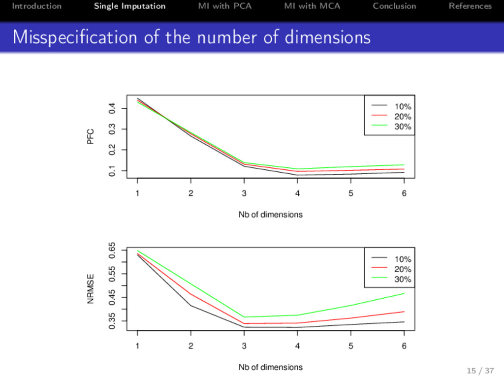
19. Introduction Single Imputation MI with PCA MI with MCA Conclusion References How to choose the number of dimensions? By cross-validation procedures: • adding missing values on the incomplete data set • predicting each of them using FAMD for several number of dimensions • calculating the prediction error Several ways: • Leave-one-out (Bro et al., 2008) • Repeated cross-validation 14 / 37
20. Introduction Single Imputation MI with PCA MI with MCA Conclusion References Misspecification of the number of dimensions 1 2 3 4 5 6 0.1 0.2 0.3 0.4 Nb of dimensions PFC 10% 20% 30% 1 2 3 4 5 6 0.35 0.45 0.55 0.65 Error on categorical variables NRMSE 10% 20% 30% 1 2 3 4 5 6 0.1 0.2 0.3 0.4 Error on categorical variables Nb of dimensions PFC 10% 20% 30% 1 2 3 4 5 6 0.35 0.45 0.55 0.65 Nb of dimensions NRMSE 10% 20% 30% 15 / 37
21. Introduction Single Imputation MI with PCA MI with MCA Conclusion References Simulation results Single imputation with FAMD shows a high quality of prediction compared to random forests (Stekhoven and Bühlmann, 2012) • on real data • when the relationships between continuous variables are linear • for rare categories • with MAR/MCAR mechanism Can impute mixed, continuous or categorical data 16 / 37
22. Introduction Single Imputation MI with PCA MI with MCA Conclusion References Simulation results Single imputation with FAMD shows a high quality of prediction compared to random forests (Stekhoven and Bühlmann, 2012) • on real data • when the relationships between continuous variables are linear • for rare categories • with MAR/MCAR mechanism Can impute mixed, continuous or categorical data But a single imputation method only 16 / 37
23. Introduction Single Imputation MI with PCA MI with MCA Conclusion References From single imputation to multiple imputation P Xmiss |Xobs , ψ1 . . . . . . . . . P Xmiss |Xobs , ψM ( ˆ F ˆ u′)ij ( ˆ F ˆ u′)1 ij + ε1 ij ( ˆ F ˆ u′)2 ij + ε2 ij ( ˆ F ˆ u′)3 ij + ε3 ij ( ˆ F ˆ u′)B ij + εB ij 1 Reflect the variability on the parameters of the imputation model → ˆ UI×S , ˆ Λ1/2 S×S , ˆ VK×S 1 , . . . , ˆ UI×S , ˆ Λ1/2 S×S , ˆ VK×S M Bayesian or Bootstrap 2 Add a disturbance on the prediction by ˆ Xm = ˆ Um ˆ Λ1/2 m ˆ Vm → need to distinguish continuous and categorical data 17 / 37
24. Introduction Single Imputation MI with PCA MI with MCA Conclusion References 1 Introduction 2 Single imputation based on principal component methods 3 Multiple imputation for continuous data with PCA 4 Multiple imputation for categorical data with MCA 5 Conclusion 18 / 37
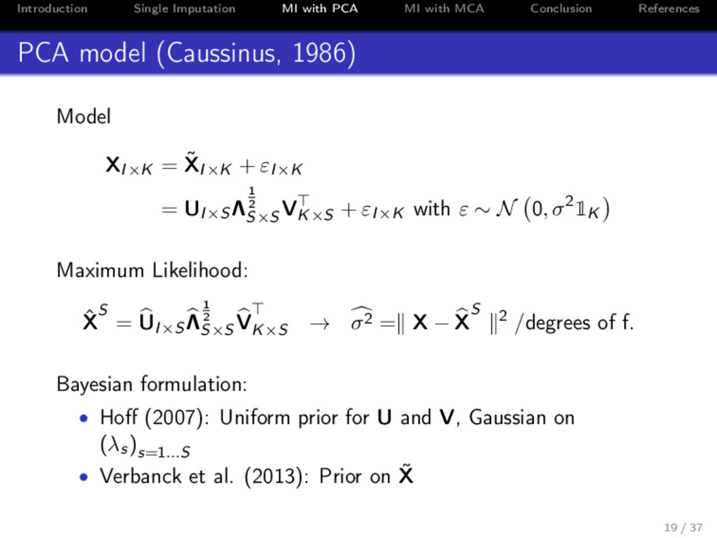
25. Introduction Single Imputation MI with PCA MI with MCA Conclusion References PCA model (Caussinus, 1986) Model XI×K = ˜ XI×K + εI×K = UI×S Λ 1 2 S×S VK×S + εI×K with ε ∼ N 0, σ21K Maximum Likelihood: ˆ XS = UI×S Λ 1 2 S×S VK×S → σ2 = X − X S 2 /degrees of f. Bayesian formulation: • Hoff (2007): Uniform prior for U and V, Gaussian on (λs)s=1...S • Verbanck et al. (2013): Prior on ˜ X 19 / 37
26. Introduction Single Imputation MI with PCA MI with MCA Conclusion References Bayesian PCA (Verbanck et al., 2013) Model: XI×K = ˜ XI×K + εI×K xik = ˜ xik + εik , εik ∼ N(0, σ2) = S s=1 √ λsuisvjs + εik = S s=1 ˜ x(s) ik + εik Prior: ˜ x(s) ik ∼ N(0, τ2 s ) Posterior: ˜ x(s) ik |x(s) ik ∼ N(Φsx(s) ik , Φsσ2) with Φs = τ2 s τ2 s +σ2 Empirical Bayes for τ2 s : ˆ τ2 s = ˆ λs − ˆ σ2 ˆ Φs = ˆ λs − ˆ σ2 ˆ λs = signal variance total variance (Efron and Morris, 1972) 20 / 37
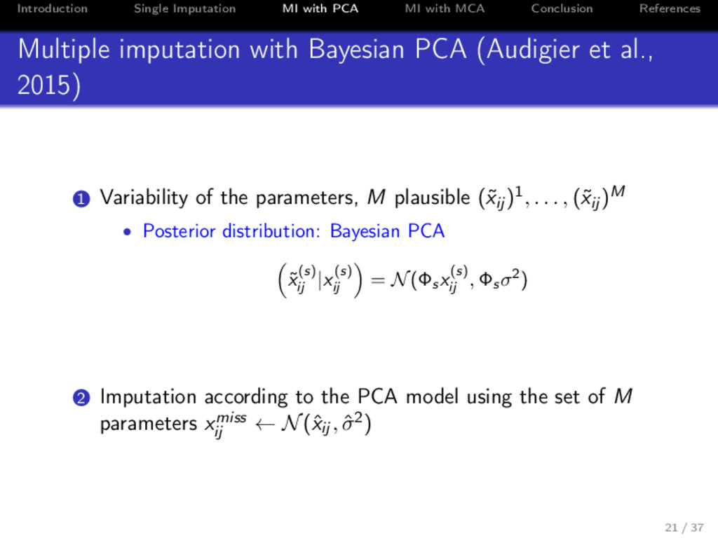
27. Introduction Single Imputation MI with PCA MI with MCA Conclusion References Multiple imputation with Bayesian PCA (Audigier et al., 2015) 1 Variability of the parameters, M plausible (˜ xij )1, . . . , (˜ xij )M • Posterior distribution: Bayesian PCA ˜ x(s) ij |x(s) ij = N(Φs x(s) ij , Φsσ2) 2 Imputation according to the PCA model using the set of M parameters xmiss ij ← N(ˆ xij , ˆ σ2) 21 / 37
28. Introduction Single Imputation MI with PCA MI with MCA Conclusion References Multiple imputation with Bayesian PCA (Audigier et al., 2015) 1 Variability of the parameters, M plausible (˜ xij )1, . . . , (˜ xij )M • Posterior distribution: Bayesian PCA ˜ x(s) ij |x(s) ij = N(Φs x(s) ij , Φsσ2) • Data Augmentation (Tanner and Wong, 1987) 2 Imputation according to the PCA model using the set of M parameters xmiss ij ← N(ˆ xij , ˆ σ2) 21 / 37
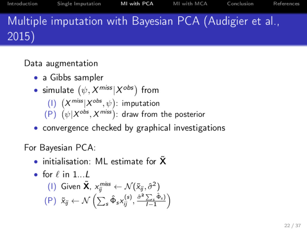
29. Introduction Single Imputation MI with PCA MI with MCA Conclusion References Multiple imputation with Bayesian PCA (Audigier et al., 2015) Data augmentation • a Gibbs sampler • simulate ψ, Xmiss|Xobs from (I) Xmiss|Xobs, ψ : imputation (P) ψ|Xobs, Xmiss : draw from the posterior • convergence checked by graphical investigations For Bayesian PCA: • initialisation: ML estimate for ˜ X • for in 1...L (I) Given ˜ X, xmiss ij ← N(˜ xij , ˆ σ2) (P) ˜ xij ← N s ˆ Φs x(s) ij , ˆ σ2 s ˆ Φs ) I−1 22 / 37
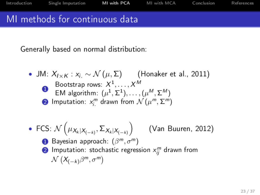
30. Introduction Single Imputation MI with PCA MI with MCA Conclusion References MI methods for continuous data Generally based on normal distribution: • JM: XI×K : xi. ∼ N (µ, Σ) (Honaker et al., 2011) 1 Bootstrap rows: X1, . . . , XM EM algorithm: (µ1, Σ1), . . . , (µM , ΣM ) 2 Imputation: xm i. drawn from N (µm, Σm) • FCS: N µXk |X(−k) , ΣXk |X(−k) (Van Buuren, 2012) 1 Bayesian approach: (βm, σm) 2 Imputation: stochastic regression xm ij drawn from N X(−k) βm, σm 23 / 37
31. Introduction Single Imputation MI with PCA MI with MCA Conclusion References Simulations • Quantities of interest: θ1 = E [Y ] , θ2 = β1, θ3 = ρ • 1000 simulations • data set drawn from Np (µ, Σ) with a two-block structure, varying I (30 or 200), K (6 or 60) and ρ (0.3 or 0.9) 0 0 0 0 0 0 0 0 0.8 0.8 0.8 0.8 0.8 0.8 0.8 0.8 0.8 0.8 0.8 0.8 0.8 0.8 0.8 0.8 • 10% or 30% of missing values using a MCAR mechanism • multiple imputation using M = 20 imputed arrays • Criteria • bias • CI width, coverage 24 / 37
32. Introduction Single Imputation MI with PCA MI with MCA Conclusion References Results for the expectation parameters confidence interval width coverage I K ρ % JM FCS BayesMIPCA JM FCS BayesMIPCA 1 30 6 0.3 0.1 0.803 0.805 0.781 0.955 0.953 0.950 2 30 6 0.3 0.3 1.010 0.898 0.971 0.949 3 30 6 0.9 0.1 0.763 0.759 0.756 0.952 0.95 0.949 4 30 6 0.9 0.3 0.818 0.783 0.965 0.953 5 30 60 0.3 0.1 0.775 0.955 6 30 60 0.3 0.3 0.864 0.952 7 30 60 0.9 0.1 0.742 0.953 8 30 60 0.9 0.3 0.759 0.954 9 200 6 0.3 0.1 0.291 0.294 0.292 0.947 0.947 0.946 10 200 6 0.3 0.3 0.328 0.334 0.325 0.954 0.959 0.952 11 200 6 0.9 0.1 0.281 0.281 0.281 0.953 0.95 0.952 12 200 6 0.9 0.3 0.288 0.289 0.288 0.948 0.951 0.951 13 200 60 0.3 0.1 0.304 0.289 0.957 0.945 14 200 60 0.3 0.3 0.384 0.313 0.981 0.958 15 200 60 0.9 0.1 0.282 0.279 0.951 0.948 16 200 60 0.9 0.3 0.296 0.283 0.958 0.952 25 / 37
33. Introduction Single Imputation MI with PCA MI with MCA Conclusion References Properties for BayesMIPCA A MI method based on a Bayesian treatment of the PCA model advantages • captures the structure of the data: good inferences for regression coefficient, correlation, mean • a dimensionality reduction method: (I < K or I > K, low or high percentage of missing values) • no inversion issue: strong or weak relationships • a regularization strategy improving stability remains competitive if: • the low rank assumption is not verified • the Gaussian assumption is not true 26 / 37
34. Introduction Single Imputation MI with PCA MI with MCA Conclusion References 1 Introduction 2 Single imputation based on principal component methods 3 Multiple imputation for continuous data with PCA 4 Multiple imputation for categorical data with MCA 5 Conclusion 27 / 37
35. Introduction Single Imputation MI with PCA MI with MCA Conclusion References Multiple imputation for categorical data using MCA MI for categorical data is very challenging for a moderate number of variables • estimation issues • storage issues 28 / 37
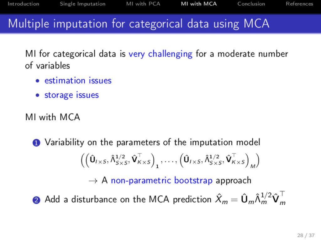
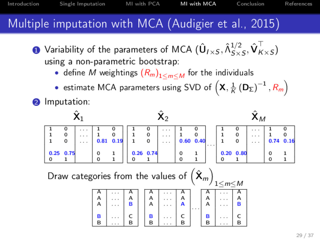
36. Introduction Single Imputation MI with PCA MI with MCA Conclusion References Multiple imputation for categorical data using MCA MI for categorical data is very challenging for a moderate number of variables • estimation issues • storage issues MI with MCA 1 Variability on the parameters of the imputation model ˆ UI×S , ˆ Λ1/2 S×S , ˆ VK×S 1 , . . . , ˆ UI×S , ˆ Λ1/2 S×S , ˆ VK×S M → A non-parametric bootstrap approach 2 Add a disturbance on the MCA prediction ˆ Xm = ˆ Um ˆ Λ1/2 m ˆ Vm 28 / 37
37. Introduction Single Imputation MI with PCA MI with MCA Conclusion References Multiple imputation with MCA (Audigier et al., 2015) 1 Variability of the parameters of MCA (ˆ UI×S , ˆ Λ1/2 S×S , ˆ VK×S ) using a non-parametric bootstrap: • define M weightings (Rm ) 1≤m≤M for the individuals • estimate MCA parameters using SVD of X, 1 K (DΣ )−1 , Rm 2 Imputation: ˆ X1 ˆ X2 ˆ XM 1 0 . . . 1 0 1 0 . . . 1 0 1 0 . . . 0.81 0.19 0.25 0.75 0 1 0 1 0 1 1 0 . . . 1 0 1 0 . . . 1 0 1 0 . . . 0.60 0.40 0.26 0.74 0 1 0 1 0 1 . . . 1 0 . . . 1 0 1 0 . . . 1 0 1 0 . . . 0.74 0.16 0.20 0.80 0 1 0 1 0 1 Draw categories from the values of ˆ Xm 1≤m≤M A . . . A A . . . A A . . . B B . . . C B . . . B A . . . A A . . . A A . . . A B . . . C B . . . B . . . A . . . A A . . . A A . . . B B . . . C B . . . B 29 / 37
38. Introduction Single Imputation MI with PCA MI with MCA Conclusion References Properties MCA address the categorical data challenge by • requiring a small number of parameters • preserving the essential data structure • using a regularisation strategy MIMCA can be applied on various data sets • small or large number of variables/categories • small or large number of individuals 30 / 37
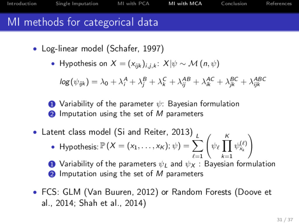
39. Introduction Single Imputation MI with PCA MI with MCA Conclusion References MI methods for categorical data • Log-linear model (Schafer, 1997) • Hypothesis on X = (xijk )i,j,k : X|ψ ∼ M (n, ψ) log(ψijk ) = λ0 + λA i + λB j + λC k + λAB ij + λAC ik + λBC jk + λABC ijk 1 Variability of the parameter ψ: Bayesian formulation 2 Imputation using the set of M parameters • Latent class model (Si and Reiter, 2013) • Hypothesis:P (X = (x1, . . . , xK ); ψ) = L =1 ψ K k=1 ψ( ) xk 1 Variability of the parameters ψL and ψX : Bayesian formulation 2 Imputation using the set of M parameters • FCS: GLM (Van Buuren, 2012) or Random Forests (Doove et al., 2014; Shah et al., 2014) 31 / 37
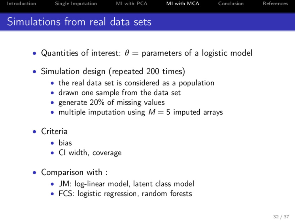
40. Introduction Single Imputation MI with PCA MI with MCA Conclusion References Simulations from real data sets • Quantities of interest: θ = parameters of a logistic model • Simulation design (repeated 200 times) • the real data set is considered as a population • drawn one sample from the data set • generate 20% of missing values • multiple imputation using M = 5 imputed arrays • Criteria • bias • CI width, coverage • Comparison with : • JM: log-linear model, latent class model • FCS: logistic regression, random forests 32 / 37
41. Introduction Single Imputation MI with PCA MI with MCA Conclusion References Results - Inference q MIMCA 5 Loglinear Latent class FCS−log FCS−rf 0.80 0.85 0.90 0.95 1.00 Titanic coverage q q q q MIMCA 2 Loglinear Latent class FCS−log FCS−rf 0.80 0.85 0.90 0.95 1.00 Galetas coverage q MIMCA 5 Latent class FCS−log FCS−rf 0.80 0.85 0.90 0.95 1.00 Income coverage Titanic Galetas Income Number of variables 4 4 14 Number of categories ≤ 4 ≤ 11 ≤ 9 33 / 37
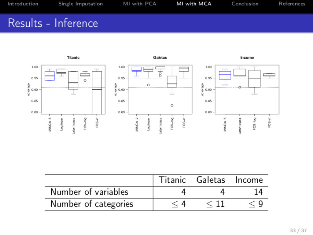
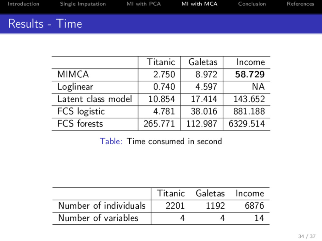
42. Introduction Single Imputation MI with PCA MI with MCA Conclusion References Results - Time Titanic Galetas Income MIMCA 2.750 8.972 58.729 Loglinear 0.740 4.597 NA Latent class model 10.854 17.414 143.652 FCS logistic 4.781 38.016 881.188 FCS forests 265.771 112.987 6329.514 Table: Time consumed in second Titanic Galetas Income Number of individuals 2201 1192 6876 Number of variables 4 4 14 34 / 37
43. Introduction Single Imputation MI with PCA MI with MCA Conclusion References Conclusion MI methods using dimensionality reduction method • captures the relationships between variables • captures the similarities between individuals • requires a small number of parameters Address some imputation issues: • can be applied on various data sets • provide correct inferences for analysis model based on relationships between pairs of variables Available in the R package missMDA 35 / 37
44. Introduction Single Imputation MI with PCA MI with MCA Conclusion References Perspectives To go further: • require a modelisation effort when categorical variables occur • for a deeper understanding of the methods • for an extension of the current methods • for a MI method based on FAMD → some lines of research: • link between CA and log-linear model • link between log-linear model and general locator model • uncertainty on the number of dimensions S 36 / 37
45. Introduction Single Imputation MI with PCA MI with MCA Conclusion References References I V. Audigier, F. Husson, and J. Josse. MIMCA: Multiple imputation for categorical variables with multiple correspondence analysis. Statistics and Computing, 2015a. Minor revision. V. Audigier, F. Husson, and J. Josse. Multiple imputation for continuous variables using a bayesian principal component analysis. Journal of Statistical Computation and Simulation, 2015b. V. Audigier, F. Husson, and J. Josse. A principal component method to impute missing values for mixed data. Advances in Data Analysis and Classification, pages 1–22, 2014. In press. D. B. Rubin. Multiple Imputation for Non-Response in Survey. Wiley, New-York, 1987. J. L. Schafer. Analysis of Incomplete Multivariate Data. Chapman & Hall/CRC, London, 1997. 37 / 37
46. Single imputation MAR • A mixed data set is simulated by splitting normal data • Missing values are added on one variable Y according to a MAR mechanism:P (Y = NA) = exp(β0+β1X1) 1+exp(β0+β1X1) • Data are imputed using FAMD and RF 1 1 1 1 1 1 1 1 1 1 1 1 1 1 1 1 1 1 1 1 1 1 1 1 1 1 1 1 1 1 1 1 1 1 1 1 1 1 1 1 1 1 1 1 1 1 1 1 1 1 1 1 1 1 1 1 1 1 1 1 1 1 1 1 1 1 1 1 1 1 1 1 1 1 1 1 1 1 1 1 1 1 1 1 1 1 1 1 1 1 1 1 1 1 1 1 1 1 1 1 1 1 1 1 1 1 1 1 1 1 1 1 1 1 1 1 1 1 1 1 1 1 1 1 1 1 1 1 1 1 1 1 1 1 1 1 1 1 1 1 1 1 1 1 1 1 1 1 1 1 1 1 1 1 1 1 1 1 1 1 1 1 1 1 1 1 1 1 1 1 1 1 1 1 1 1 1 1 1 1 1 1 1 1 1 1 1 1 1 1 1 1 1 1 1 1 1 1 1 1 1 1 1 1 1 1 1 1 1 1 1 1 1 1 1 1 1 1 1 1 1 1 1 1 1 1 1 1 1 1 1 1 1 1 1 1 1 1 1 1 1 1 1 1 1 1 1 1 1 1 1 1 1 1 1 1 1 1 1 1 1 1 1 1 1 1 1 1 1 1 1 1 1 1 1 1 1 1 1 1 1 1 1 1 1 1 1 1 1 1 1 1 1 1 1 1 1 1 1 1 1 1 1 1 1 1 1 1 1 1 1 1 1 1 1 1 1 1 1 1 1 1 1 1 1 1 1 1 1 1 1 1 1 1 1 1 1 1 1 1 1 1 1 1 1 1 1 1 1 1 1 1 1 1 1 1 1 1 1 1 1 1 1 1 1 1 1 1 1 1 1 1 1 1 1 1 1 1 1 1 1 1 1 1 1 1 1 1 1 1 1 1 1 1 1 1 1 1 1 1 1 1 1 1 1 1 1 1 1 1 1 1 1 1 1 1 1 1 1 1 1 1 1 1 1 1 1 1 1 1 1 1 1 1 1 1 1 1 1 1 1 1 1 1 1 1 1 1 1 1 1 1 1 1 1 1 1 1 1 1 1 1 1 1 1 1 1 1 1 1 1 1 1 1 1 1 1 1 1 1 1 1 1 1 1 1 1 1 1 1 1 1 1 1 1 1 1 1 1 1 1 1 1 1 1 1 1 1 1 1 1 1 1 1 1 1 1 1 1 1 1 1 1 1 1 1 1 1 1 1 1 1 1 1 1 1 1 1 1 1 1 1 1 1 1 1 1 1 1 1 1 1 1 1 1 1 1 1 1 1 1 1 1 1 1 1 1 1 1 1 1 1 1 1 1 1 1 1 1 1 1 1 1 1 1 1 1 1 1 1 1 1 1 1 1 1 1 1 1 1 1 1 1 1 1 1 1 1 1 1 1 1 1 1 1 1 1 1 1 1 1 1 1 1 1 1 1 1 1 1 1 1 1 1 1 1 1 1 1 1 1 1 1 1 1 1 1 1 1 1 1 1 1 1 1 1 1 1 1 1 1 1 1 1 1 1 1 1 1 1 1 1 1 1 1 1 1 1 1 1 1 1 1 1 1 1 1 1 1 1 1 1 1 1 1 1 1 1 1 1 1 1 1 1 1 1 1 1 1 1 1 1 1 1 1 1 1 1 1 1 1 1 1 1 1 1 1 1 1 1 1 1 1 1 1 1 1 1 1 1 1 1 1 1 1 1 1 1 1 1 1 1 1 1 1 1 1 1 1 1 1 1 1 1 1 1 1 1 1 1 1 1 1 1 1 1 1 1 1 1 1 1 1 1 1 1 1 1 1 1 1 1 1 1 1 1 1 1 1 1 1 1 1 1 1 1 1 1 1 1 1 1 1 1 1 1 1 1 1 1 1 1 1 1 1 1 1 1 1 1 1 1 1 1 1 1 1 1 1 1 1 1 1 1 1 1 1 1 1 1 1 1 1 1 1 1 1 1 1 1 1 1 1 1 1 1 1 1 1 1 1 1 1 1 1 1 1 1 1 1 1 1 1 1 1 1 1 1 1 1 1 1 1 1 1 1 1 1 1 1 1 1 1 1 1 1 1 1 1 1 1 1 1 1 1 1 1 1 1 1 1 1 1 1 1 1 1 1 1 1 1 1 1 1 1 1 1 1 1 1 1 1 1 1 1 1 1 1 1 1 1 1 1 1 1 1 1 1 1 1 1 1 1 1 1 1 1 1 1 1 1 1 1 1 1 1 1 1 1 1 1 1 1 1 1 1 1 1 1 1 1 1 1 1 1 1 1 1 1 1 1 −4 −2 0 2 4 0.0 0.2 0.4 0.6 0.8 1.0 x P(y=NA) 2 2 2 2 2 2 2 2 2 2 2 2 2 2 2 2 2 2 2 2 2 2 2 2 2 2 2 2 2 2 2 2 2 2 2 2 2 2 2 2 2 2 2 2 2 2 2 2 2 2 2 2 2 2 2 2 2 2 2 2 2 2 2 2 2 2 2 2 2 2 2 2 2 2 2 2 2 2 2 2 2 2 2 2 2 2 2 2 2 2 2 2 2 2 2 2 2 2 2 2 2 2 2 2 2 2 2 2 2 2 2 2 2 2 2 2 2 2 2 2 2 2 2 2 2 2 2 2 2 2 2 2 2 2 2 2 2 2 2 2 2 2 2 2 2 2 2 2 2 2 2 2 2 2 2 2 2 2 2 2 2 2 2 2 2 2 2 2 2 2 2 2 2 2 2 2 2 2 2 2 2 2 2 2 2 2 2 2 2 2 2 2 2 2 2 2 2 2 2 2 2 2 2 2 2 2 2 2 2 2 2 2 2 2 2 2 2 2 2 2 2 2 2 2 2 2 2 2 2 2 2 2 2 2 2 2 2 2 2 2 2 2 2 2 2 2 2 2 2 2 2 2 2 2 2 2 2 2 2 2 2 2 2 2 2 2 2 2 2 2 2 2 2 2 2 2 2 2 2 2 2 2 2 2 2 2 2 2 2 2 2 2 2 2 2 2 2 2 2 2 2 2 2 2 2 2 2 2 2 2 2 2 2 2 2 2 2 2 2 2 2 2 2 2 2 2 2 2 2 2 2 2 2 2 2 2 2 2 2 2 2 2 2 2 2 2 2 2 2 2 2 2 2 2 2 2 2 2 2 2 2 2 2 2 2 2 2 2 2 2 2 2 2 2 2 2 2 2 2 2 2 2 2 2 2 2 2 2 2 2 2 2 2 2 2 2 2 2 2 2 2 2 2 2 2 2 2 2 2 2 2 2 2 2 2 2 2 2 2 2 2 2 2 2 2 2 2 2 2 2 2 2 2 2 2 2 2 2 2 2 2 2 2 2 2 2 2 2 2 2 2 2 2 2 2 2 2 2 2 2 2 2 2 2 2 2 2 2 2 2 2 2 2 2 2 2 2 2 2 2 2 2 2 2 2 2 2 2 2 2 2 2 2 2 2 2 2 2 2 2 2 2 2 2 2 2 2 2 2 2 2 2 2 2 2 2 2 2 2 2 2 2 2 2 2 2 2 2 2 2 2 2 2 2 2 2 2 2 2 2 2 2 2 2 2 2 2 2 2 2 2 2 2 2 2 2 2 2 2 2 2 2 2 2 2 2 2 2 2 2 2 2 2 2 2 2 2 2 2 2 2 2 2 2 2 2 2 2 2 2 2 2 2 2 2 2 2 2 2 2 2 2 2 2 2 2 2 2 2 2 2 2 2 2 2 2 2 2 2 2 2 2 2 2 2 2 2 2 2 2 2 2 2 2 2 2 2 2 2 2 2 2 2 2 2 2 2 2 2 2 2 2 2 2 2 2 2 2 2 2 2 2 2 2 2 2 2 2 2 2 2 2 2 2 2 2 2 2 2 2 2 2 2 2 2 2 2 2 2 2 2 2 2 2 2 2 2 2 2 2 2 2 2 2 2 2 2 2 2 2 2 2 2 2 2 2 2 2 2 2 2 2 2 2 2 2 2 2 2 2 2 2 2 2 2 2 2 2 2 2 2 2 2 2 2 2 2 2 2 2 2 2 2 2 2 2 2 2 2 2 2 2 2 2 2 2 2 2 2 2 2 2 2 2 2 2 2 2 2 2 2 2 2 2 2 2 2 2 2 2 2 2 2 2 2 2 2 2 2 2 2 2 2 2 2 2 2 2 2 2 2 2 2 2 2 2 2 2 2 2 2 2 2 2 2 2 2 2 2 2 2 2 2 2 2 2 2 2 2 2 2 2 2 2 2 2 2 2 2 2 2 2 2 2 2 2 2 2 2 2 2 2 2 2 2 2 2 2 2 2 2 2 2 2 2 2 2 2 2 2 2 2 2 2 2 2 2 2 2 2 2 2 2 2 2 2 2 2 2 2 2 2 2 2 2 2 2 2 2 2 2 2 2 2 2 2 2 2 2 2 2 2 2 2 2 2 2 2 2 2 2 2 2 2 2 2 2 2 2 2 2 2 2 2 2 2 2 2 2 2 2 2 2 2 2 2 2 2 2 2 2 2 2 2 2 2 2 2 2 2 2 2 2 2 2 2 2 2 2 2 2 2 2 2 2 2 2 2 2 2 2 2 2 2 2 2 2 2 2 2 2 3 3 3 3 3 3 3 3 3 3 3 3 3 3 3 3 3 3 3 3 3 3 3 3 3 3 3 3 3 3 3 3 3 3 3 3 3 3 3 3 3 3 3 3 3 3 3 3 3 3 3 3 3 3 3 3 3 3 3 3 3 3 3 3 3 3 3 3 3 3 3 3 3 3 3 3 3 3 3 3 3 3 3 3 3 3 3 3 3 3 3 3 3 3 3 3 3 3 3 3 3 3 3 3 3 3 3 3 3 3 3 3 3 3 3 3 3 3 3 3 3 3 3 3 3 3 3 3 3 3 3 3 3 3 3 3 3 3 3 3 3 3 3 3 3 3 3 3 3 3 3 3 3 3 3 3 3 3 3 3 3 3 3 3 3 3 3 3 3 3 3 3 3 3 3 3 3 3 3 3 3 3 3 3 3 3 3 3 3 3 3 3 3 3 3 3 3 3 3 3 3 3 3 3 3 3 3 3 3 3 3 3 3 3 3 3 3 3 3 3 3 3 3 3 3 3 3 3 3 3 3 3 3 3 3 3 3 3 3 3 3 3 3 3 3 3 3 3 3 3 3 3 3 3 3 3 3 3 3 3 3 3 3 3 3 3 3 3 3 3 3 3 3 3 3 3 3 3 3 3 3 3 3 3 3 3 3 3 3 3 3 3 3 3 3 3 3 3 3 3 3 3 3 3 3 3 3 3 3 3 3 3 3 3 3 3 3 3 3 3 3 3 3 3 3 3 3 3 3 3 3 3 3 3 3 3 3 3 3 3 3 3 3 3 3 3 3 3 3 3 3 3 3 3 3 3 3 3 3 3 3 3 3 3 3 3 3 3 3 3 3 3 3 3 3 3 3 3 3 3 3 3 3 3 3 3 3 3 3 3 3 3 3 3 3 3 3 3 3 3 3 3 3 3 3 3 3 3 3 3 3 3 3 3 3 3 3 3 3 3 3 3 3 3 3 3 3 3 3 3 3 3 3 3 3 3 3 3 3 3 3 3 3 3 3 3 3 3 3 3 3 3 3 3 3 3 3 3 3 3 3 3 3 3 3 3 3 3 3 3 3 3 3 3 3 3 3 3 3 3 3 3 3 3 3 3 3 3 3 3 3 3 3 3 3 3 3 3 3 3 3 3 3 3 3 3 3 3 3 3 3 3 3 3 3 3 3 3 3 3 3 3 3 3 3 3 3 3 3 3 3 3 3 3 3 3 3 3 3 3 3 3 3 3 3 3 3 3 3 3 3 3 3 3 3 3 3 3 3 3 3 3 3 3 3 3 3 3 3 3 3 3 3 3 3 3 3 3 3 3 3 3 3 3 3 3 3 3 3 3 3 3 3 3 3 3 3 3 3 3 3 3 3 3 3 3 3 3 3 3 3 3 3 3 3 3 3 3 3 3 3 3 3 3 3 3 3 3 3 3 3 3 3 3 3 3 3 3 3 3 3 3 3 3 3 3 3 3 3 3 3 3 3 3 3 3 3 3 3 3 3 3 3 3 3 3 3 3 3 3 3 3 3 3 3 3 3 3 3 3 3 3 3 3 3 3 3 3 3 3 3 3 3 3 3 3 3 3 3 3 3 3 3 3 3 3 3 3 3 3 3 3 3 3 3 3 3 3 3 3 3 3 3 3 3 3 3 3 3 3 3 3 3 3 3 3 3 3 3 3 3 3 3 3 3 3 3 3 3 3 3 3 3 3 3 3 3 3 3 3 3 3 3 3 3 3 3 3 3 3 3 3 3 3 3 3 3 3 3 3 3 3 3 3 3 3 3 3 3 3 3 3 3 3 3 3 3 3 3 3 3 3 3 3 3 3 3 3 3 3 3 3 3 3 3 3 3 3 3 3 3 3 3 3 3 3 3 3 3 3 3 3 3 3 3 3 3 3 3 3 3 3 3 3 3 3 3 3 3 3 3 3 3 3 3 3 3 3 3 3 3 3 3 3 3 3 3 3 3 3 3 3 3 3 3 3 3 3 3 3 3 3 3 3 3 3 3 3 3 3 3 3 3 3 3 3 3 3 3 3 3 3 3 3 3 3 3 3 3 3 3 3 3 3 3 3 3 3 3 3 3 3 3 3 3 3 3 3 3 3 3 3 3 3 3 3 3 3 3 3 3 3 3 3 3 3 3 3 3 3 3 3 3 3 3 3 3 3 3 3 3 3 3 3 3 3 3 3 3 3 3 3 3 3 3 3 3 3 3 3 3 3 3 3 3 3 3 3 3 3 3 3 3 3 3 3 3 3 3 3 3 4 4 4 4 4 4 4 4 4 4 4 4 4 4 4 4 4 4 4 4 4 4 4 4 4 4 4 4 4 4 4 4 4 4 4 4 4 4 4 4 4 4 4 4 4 4 4 4 4 4 4 4 4 4 4 4 4 4 4 4 4 4 4 4 4 4 4 4 4 4 4 4 4 4 4 4 4 4 4 4 4 4 4 4 4 4 4 4 4 4 4 4 4 4 4 4 4 4 4 4 4 4 4 4 4 4 4 4 4 4 4 4 4 4 4 4 4 4 4 4 4 4 4 4 4 4 4 4 4 4 4 4 4 4 4 4 4 4 4 4 4 4 4 4 4 4 4 4 4 4 4 4 4 4 4 4 4 4 4 4 4 4 4 4 4 4 4 4 4 4 4 4 4 4 4 4 4 4 4 4 4 4 4 4 4 4 4 4 4 4 4 4 4 4 4 4 4 4 4 4 4 4 4 4 4 4 4 4 4 4 4 4 4 4 4 4 4 4 4 4 4 4 4 4 4 4 4 4 4 4 4 4 4 4 4 4 4 4 4 4 4 4 4 4 4 4 4 4 4 4 4 4 4 4 4 4 4 4 4 4 4 4 4 4 4 4 4 4 4 4 4 4 4 4 4 4 4 4 4 4 4 4 4 4 4 4 4 4 4 4 4 4 4 4 4 4 4 4 4 4 4 4 4 4 4 4 4 4 4 4 4 4 4 4 4 4 4 4 4 4 4 4 4 4 4 4 4 4 4 4 4 4 4 4 4 4 4 4 4 4 4 4 4 4 4 4 4 4 4 4 4 4 4 4 4 4 4 4 4 4 4 4 4 4 4 4 4 4 4 4 4 4 4 4 4 4 4 4 4 4 4 4 4 4 4 4 4 4 4 4 4 4 4 4 4 4 4 4 4 4 4 4 4 4 4 4 4 4 4 4 4 4 4 4 4 4 4 4 4 4 4 4 4 4 4 4 4 4 4 4 4 4 4 4 4 4 4 4 4 4 4 4 4 4 4 4 4 4 4 4 4 4 4 4 4 4 4 4 4 4 4 4 4 4 4 4 4 4 4 4 4 4 4 4 4 4 4 4 4 4 4 4 4 4 4 4 4 4 4 4 4 4 4 4 4 4 4 4 4 4 4 4 4 4 4 4 4 4 4 4 4 4 4 4 4 4 4 4 4 4 4 4 4 4 4 4 4 4 4 4 4 4 4 4 4 4 4 4 4 4 4 4 4 4 4 4 4 4 4 4 4 4 4 4 4 4 4 4 4 4 4 4 4 4 4 4 4 4 4 4 4 4 4 4 4 4 4 4 4 4 4 4 4 4 4 4 4 4 4 4 4 4 4 4 4 4 4 4 4 4 4 4 4 4 4 4 4 4 4 4 4 4 4 4 4 4 4 4 4 4 4 4 4 4 4 4 4 4 4 4 4 4 4 4 4 4 4 4 4 4 4 4 4 4 4 4 4 4 4 4 4 4 4 4 4 4 4 4 4 4 4 4 4 4 4 4 4 4 4 4 4 4 4 4 4 4 4 4 4 4 4 4 4 4 4 4 4 4 4 4 4 4 4 4 4 4 4 4 4 4 4 4 4 4 4 4 4 4 4 4 4 4 4 4 4 4 4 4 4 4 4 4 4 4 4 4 4 4 4 4 4 4 4 4 4 4 4 4 4 4 4 4 4 4 4 4 4 4 4 4 4 4 4 4 4 4 4 4 4 4 4 4 4 4 4 4 4 4 4 4 4 4 4 4 4 4 4 4 4 4 4 4 4 4 4 4 4 4 4 4 4 4 4 4 4 4 4 4 4 4 4 4 4 4 4 4 4 4 4 4 4 4 4 4 4 4 4 4 4 4 4 4 4 4 4 4 4 4 4 4 4 4 4 4 4 4 4 4 4 4 4 4 4 4 4 4 4 4 4 4 4 4 4 4 4 4 4 4 4 4 4 4 4 4 4 4 4 4 4 4 4 4 4 4 4 4 4 4 4 4 4 4 4 4 4 4 4 4 4 4 4 4 4 4 4 4 4 4 4 4 4 4 4 4 4 4 4 4 4 4 4 4 4 4 4 4 4 4 4 4 4 4 4 4 4 4 4 4 4 4 4 4 4 4 4 4 4 4 4 4 4 4 4 4 4 4 4 4 4 4 4 4 4 4 4 4 4 4 4 4 4 4 4 4 4 4 4 4 4 4 4 4 4 4 4 4 4 4 4 4 4 4 4 4 4 4 4 4 4 4 4 4 4 4 4 4 4 4 4 4 4 5 5 5 5 5 5 5 5 5 5 5 5 5 5 5 5 5 5 5 5 5 5 5 5 5 5 5 5 5 5 5 5 5 5 5 5 5 5 5 5 5 5 5 5 5 5 5 5 5 5 5 5 5 5 5 5 5 5 5 5 5 5 5 5 5 5 5 5 5 5 5 5 5 5 5 5 5 5 5 5 5 5 5 5 5 5 5 5 5 5 5 5 5 5 5 5 5 5 5 5 5 5 5 5 5 5 5 5 5 5 5 5 5 5 5 5 5 5 5 5 5 5 5 5 5 5 5 5 5 5 5 5 5 5 5 5 5 5 5 5 5 5 5 5 5 5 5 5 5 5 5 5 5 5 5 5 5 5 5 5 5 5 5 5 5 5 5 5 5 5 5 5 5 5 5 5 5 5 5 5 5 5 5 5 5 5 5 5 5 5 5 5 5 5 5 5 5 5 5 5 5 5 5 5 5 5 5 5 5 5 5 5 5 5 5 5 5 5 5 5 5 5 5 5 5 5 5 5 5 5 5 5 5 5 5 5 5 5 5 5 5 5 5 5 5 5 5 5 5 5 5 5 5 5 5 5 5 5 5 5 5 5 5 5 5 5 5 5 5 5 5 5 5 5 5 5 5 5 5 5 5 5 5 5 5 5 5 5 5 5 5 5 5 5 5 5 5 5 5 5 5 5 5 5 5 5 5 5 5 5 5 5 5 5 5 5 5 5 5 5 5 5 5 5 5 5 5 5 5 5 5 5 5 5 5 5 5 5 5 5 5 5 5 5 5 5 5 5 5 5 5 5 5 5 5 5 5 5 5 5 5 5 5 5 5 5 5 5 5 5 5 5 5 5 5 5 5 5 5 5 5 5 5 5 5 5 5 5 5 5 5 5 5 5 5 5 5 5 5 5 5 5 5 5 5 5 5 5 5 5 5 5 5 5 5 5 5 5 5 5 5 5 5 5 5 5 5 5 5 5 5 5 5 5 5 5 5 5 5 5 5 5 5 5 5 5 5 5 5 5 5 5 5 5 5 5 5 5 5 5 5 5 5 5 5 5 5 5 5 5 5 5 5 5 5 5 5 5 5 5 5 5 5 5 5 5 5 5 5 5 5 5 5 5 5 5 5 5 5 5 5 5 5 5 5 5 5 5 5 5 5 5 5 5 5 5 5 5 5 5 5 5 5 5 5 5 5 5 5 5 5 5 5 5 5 5 5 5 5 5 5 5 5 5 5 5 5 5 5 5 5 5 5 5 5 5 5 5 5 5 5 5 5 5 5 5 5 5 5 5 5 5 5 5 5 5 5 5 5 5 5 5 5 5 5 5 5 5 5 5 5 5 5 5 5 5 5 5 5 5 5 5 5 5 5 5 5 5 5 5 5 5 5 5 5 5 5 5 5 5 5 5 5 5 5 5 5 5 5 5 5 5 5 5 5 5 5 5 5 5 5 5 5 5 5 5 5 5 5 5 5 5 5 5 5 5 5 5 5 5 5 5 5 5 5 5 5 5 5 5 5 5 5 5 5 5 5 5 5 5 5 5 5 5 5 5 5 5 5 5 5 5 5 5 5 5 5 5 5 5 5 5 5 5 5 5 5 5 5 5 5 5 5 5 5 5 5 5 5 5 5 5 5 5 5 5 5 5 5 5 5 5 5 5 5 5 5 5 5 5 5 5 5 5 5 5 5 5 5 5 5 5 5 5 5 5 5 5 5 5 5 5 5 5 5 5 5 5 5 5 5 5 5 5 5 5 5 5 5 5 5 5 5 5 5 5 5 5 5 5 5 5 5 5 5 5 5 5 5 5 5 5 5 5 5 5 5 5 5 5 5 5 5 5 5 5 5 5 5 5 5 5 5 5 5 5 5 5 5 5 5 5 5 5 5 5 5 5 5 5 5 5 5 5 5 5 5 5 5 5 5 5 5 5 5 5 5 5 5 5 5 5 5 5 5 5 5 5 5 5 5 5 5 5 5 5 5 5 5 5 5 5 5 5 5 5 5 5 5 5 5 5 5 5 5 5 5 5 5 5 5 5 5 5 5 5 5 5 5 5 5 5 5 5 5 5 5 5 5 5 5 5 5 5 5 5 5 5 5 5 5 5 5 5 5 5 5 5 5 5 5 5 5 5 5 5 5 5 5 5 5 5 5 5 5 5 5 5 5 5 5 5 5 5 5 5 5 5 5 5 5 5 5 5 5 5 5 5 5 5 5 5 5 5 5 5 5 5 5 5 5 5 5 5 5 5 5 5 5 5 5 6 6 6 6 6 6 6 6 6 6 6 6 6 6 6 6 6 6 6 6 6 6 6 6 6 6 6 6 6 6 6 6 6 6 6 6 6 6 6 6 6 6 6 6 6 6 6 6 6 6 6 6 6 6 6 6 6 6 6 6 6 6 6 6 6 6 6 6 6 6 6 6 6 6 6 6 6 6 6 6 6 6 6 6 6 6 6 6 6 6 6 6 6 6 6 6 6 6 6 6 6 6 6 6 6 6 6 6 6 6 6 6 6 6 6 6 6 6 6 6 6 6 6 6 6 6 6 6 6 6 6 6 6 6 6 6 6 6 6 6 6 6 6 6 6 6 6 6 6 6 6 6 6 6 6 6 6 6 6 6 6 6 6 6 6 6 6 6 6 6 6 6 6 6 6 6 6 6 6 6 6 6 6 6 6 6 6 6 6 6 6 6 6 6 6 6 6 6 6 6 6 6 6 6 6 6 6 6 6 6 6 6 6 6 6 6 6 6 6 6 6 6 6 6 6 6 6 6 6 6 6 6 6 6 6 6 6 6 6 6 6 6 6 6 6 6 6 6 6 6 6 6 6 6 6 6 6 6 6 6 6 6 6 6 6 6 6 6 6 6 6 6 6 6 6 6 6 6 6 6 6 6 6 6 6 6 6 6 6 6 6 6 6 6 6 6 6 6 6 6 6 6 6 6 6 6 6 6 6 6 6 6 6 6 6 6 6 6 6 6 6 6 6 6 6 6 6 6 6 6 6 6 6 6 6 6 6 6 6 6 6 6 6 6 6 6 6 6 6 6 6 6 6 6 6 6 6 6 6 6 6 6 6 6 6 6 6 6 6 6 6 6 6 6 6 6 6 6 6 6 6 6 6 6 6 6 6 6 6 6 6 6 6 6 6 6 6 6 6 6 6 6 6 6 6 6 6 6 6 6 6 6 6 6 6 6 6 6 6 6 6 6 6 6 6 6 6 6 6 6 6 6 6 6 6 6 6 6 6 6 6 6 6 6 6 6 6 6 6 6 6 6 6 6 6 6 6 6 6 6 6 6 6 6 6 6 6 6 6 6 6 6 6 6 6 6 6 6 6 6 6 6 6 6 6 6 6 6 6 6 6 6 6 6 6 6 6 6 6 6 6 6 6 6 6 6 6 6 6 6 6 6 6 6 6 6 6 6 6 6 6 6 6 6 6 6 6 6 6 6 6 6 6 6 6 6 6 6 6 6 6 6 6 6 6 6 6 6 6 6 6 6 6 6 6 6 6 6 6 6 6 6 6 6 6 6 6 6 6 6 6 6 6 6 6 6 6 6 6 6 6 6 6 6 6 6 6 6 6 6 6 6 6 6 6 6 6 6 6 6 6 6 6 6 6 6 6 6 6 6 6 6 6 6 6 6 6 6 6 6 6 6 6 6 6 6 6 6 6 6 6 6 6 6 6 6 6 6 6 6 6 6 6 6 6 6 6 6 6 6 6 6 6 6 6 6 6 6 6 6 6 6 6 6 6 6 6 6 6 6 6 6 6 6 6 6 6 6 6 6 6 6 6 6 6 6 6 6 6 6 6 6 6 6 6 6 6 6 6 6 6 6 6 6 6 6 6 6 6 6 6 6 6 6 6 6 6 6 6 6 6 6 6 6 6 6 6 6 6 6 6 6 6 6 6 6 6 6 6 6 6 6 6 6 6 6 6 6 6 6 6 6 6 6 6 6 6 6 6 6 6 6 6 6 6 6 6 6 6 6 6 6 6 6 6 6 6 6 6 6 6 6 6 6 6 6 6 6 6 6 6 6 6 6 6 6 6 6 6 6 6 6 6 6 6 6 6 6 6 6 6 6 6 6 6 6 6 6 6 6 6 6 6 6 6 6 6 6 6 6 6 6 6 6 6 6 6 6 6 6 6 6 6 6 6 6 6 6 6 6 6 6 6 6 6 6 6 6 6 6 6 6 6 6 6 6 6 6 6 6 6 6 6 6 6 6 6 6 6 6 6 6 6 6 6 6 6 6 6 6 6 6 6 6 6 6 6 6 6 6 6 6 6 6 6 6 6 6 6 6 6 6 6 6 6 6 6 6 6 6 6 6 6 6 6 6 6 6 6 6 6 6 6 6 6 6 6 6 6 6 6 6 6 6 6 6 6 6 6 6 6 6 6 6 6 6 6 6 6 6 6 6 6 6 6 6 6 6 6 6 6 6 6 6 6 6 6 6 6 6 6 6 6 6 6 6 6 6 6 6 6 6 6 6 6 6 6 6 6 6 6 beta=0 beta=0.2 beta=0.4 beta=0.6 beta=0.8 beta=1 0 1 2 3 4 0.2 0.3 0.4 0.5 0.6 0.7 beta NRMSE RF FAMD 0 1 2 3 4 0.00 0.10 0.20 PFC RF FAMD