Visualization/ellipses PCA

Transcript

1. Introduction Low-rank matrix estimation Confidence areas Bayesian Data visualization with Principal Component Analysis Julie Josse Statistics Department, Agronomy University Agrocampus, Rennes, France Workshop in Biostatistics, Stanford University, 15 January 2015 1 / 57
2. Introduction Low-rank matrix estimation Confidence areas Bayesian Outline 1. Plant-Breeding example 2. Regularized low rank matrix estimation • Singular-values shrinkage • Parametric bootstrap approach 3. Confidence areas for biplots: bootstrap/jaccknife 4. Bayesian treatment of SVD models 2 / 57
3. Introduction Low-rank matrix estimation Confidence areas Bayesian Genotypes - Environement data 16 triticales (6 complete - 8 substituted - 2 checks) 10 locations in Spain (heterogeneous pH) ⇒ Adaptation of the triticales to the Spanish soil ⇒ AMMI (Additive Main effects and Multiplicative Interaction) yij = µ + αi + βj + k l=1 dl uil vjl + εij Y11 G1 E1    Y1J Y21    YIJ    G1 G2    GI    EJ E2    EJ Y G E G1      GI       YJ       E1 EJ ⇒ PCA on the residuals matrix of the 2-way anova 3 / 57
4. Introduction Low-rank matrix estimation Confidence areas Bayesian Principal Component Analysis ⇒ Do the genotypes have different performances in different environments? −3 −2 −1 0 1 2 3 −2 −1 0 1 2 3 Genotypes Dim 1 (71.44%) Dim 2 (16.40%) C_1 C_2 C_3 C_4 C_5 C_6 S_1 S_2 S_3 S_4 S_5 S_6 S_7 S_8 S_F S_M −1.0 −0.5 0.0 0.5 −0.5 0.0 0.5 Variables factor map (PCA) Dim 1 (71.44%) Dim 2 (16.40%) ALBACETE BADAJOZ CORDOBA CORUNA LLEIDA ORENSE SALAMANCA SEVILLA TOLEDO SEVILLA_2 ALBACETE BADAJOZ CORDOBA CORUNA LLEIDA ORENSE SALAMANCA SEVILLA TOLEDO SEVILLA_2 ALBACETE BADAJOZ CORDOBA CORUNA LLEIDA ORENSE SALAMANCA SEVILLA TOLEDO SEVILLA_2 ALBACETE BADAJOZ CORDOBA CORUNA LLEIDA ORENSE SALAMANCA SEVILLA TOLEDO SEVILLA_2 ALBACETE BADAJOZ CORDOBA CORUNA LLEIDA ORENSE SALAMANCA SEVILLA TOLEDO SEVILLA_2 ALBACETE BADAJOZ CORDOBA CORUNA LLEIDA ORENSE SALAMANCA SEVILLA TOLEDO SEVILLA_2 ALBACETE BADAJOZ CORDOBA CORUNA LLEIDA ORENSE SALAMANCA SEVILLA TOLEDO SEVILLA_2 ALBACETE BADAJOZ CORDOBA CORUNA LLEIDA ORENSE SALAMANCA SEVILLA TOLEDO SEVILLA_2 ALBACETE BADAJOZ CORDOBA CORUNA LLEIDA ORENSE SALAMANCA SEVILLA TOLEDO SEVILLA_2 Scores F = UD1/2 and variables coordinates VD1/2 ⇒ Opposition Complete (C) and Substituted (S) 4 / 57
5. Introduction Low-rank matrix estimation Confidence areas Bayesian Clustering on PC 0.0 1.0 2.0 Hierarchical clustering inertia gain S_1 C_1 S_M C_2 C_6 C_4 C_5 C_3 S_4 S_5 S_6 S_3 S_F S_7 S_8 S_2 0.0 0.5 1.0 1.5 2.0 Cluster Dendrogram Height −3 −2 −1 0 1 2 3 −1 0 1 2 clustering Dim 1 (71.44%) Dim 2 (16.40%) C_2 C_4 C_6 C_5 C_3 C_1 S_M S_1 S_F S_7 S_5 S_3 S_6 S_8 S_2 S_4 cluster 1 cluster 2 cluster 3 cluster 4 cluster 1 cluster 2 cluster 3 cluster 4 Clustering on the denoised matrix ˆ µk = k l=1 ul dl v l 5 / 57
6. Introduction Low-rank matrix estimation Confidence areas Bayesian Low-rank matrix estimation ⇒ Gaussian noise model Xn×p = µ + ε, with εij iid ∼ N 0, σ2 with µ of low rank k Image, collaborative filtering... ⇒ Classical solution: truncated SVD ˆ µk = k l=1 ul dl v l Hard thresholding: dl · 1(l ≤ k) = dl · 1(dl ≥ λ) argminµ X − µ 2 2 : rank (µ) ≤ k ⇒ Selecting k? Cross-validation (Josse & Husson, 2012) 6 / 57
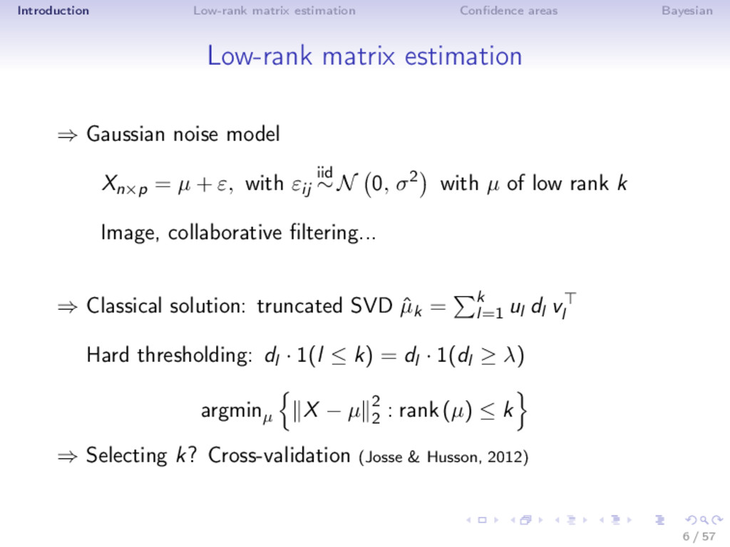
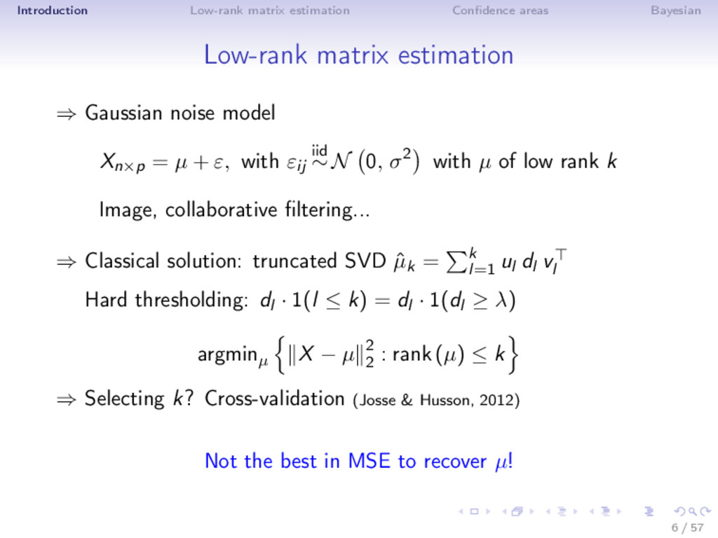
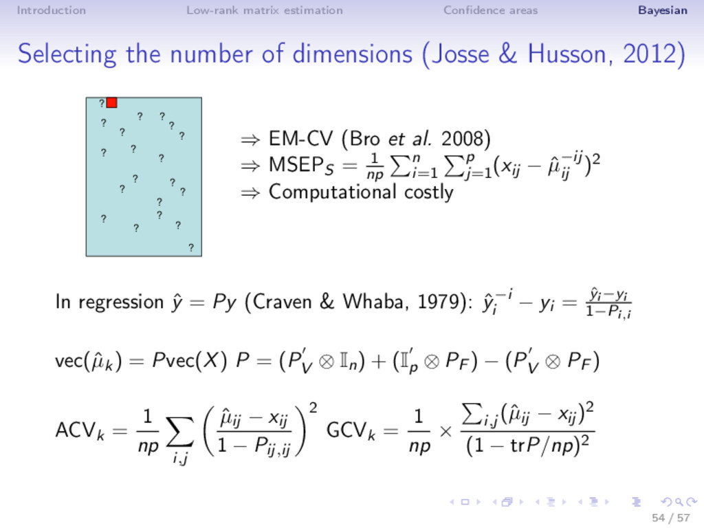
7. Introduction Low-rank matrix estimation Confidence areas Bayesian Low-rank matrix estimation ⇒ Gaussian noise model Xn×p = µ + ε, with εij iid ∼ N 0, σ2 with µ of low rank k Image, collaborative filtering... ⇒ Classical solution: truncated SVD ˆ µk = k l=1 ul dl v l Hard thresholding: dl · 1(l ≤ k) = dl · 1(dl ≥ λ) argminµ X − µ 2 2 : rank (µ) ≤ k ⇒ Selecting k? Cross-validation (Josse & Husson, 2012) Not the best in MSE to recover µ! 6 / 57
8. Introduction Low-rank matrix estimation Confidence areas Bayesian Outline 1. Plant-Breeding example 2. Regularized low rank matrix estimation • Singular-values shrinkers • Bootstrap approach 3. Confidence areas for biplots: bootstrap/jaccknife 4. Bayesian treatment of SVD models 7 / 57
9. Introduction Low-rank matrix estimation Confidence areas Bayesian Shrinking - thresholding SVD ⇒ Soft threshoding: dl max 1 − λ dl , 0 argminµ X − µ 2 2 + λ µ ∗ ⇒ Selecting λ? MSE(λ) = E µ − ˆ µλ 2 Stein’s Unbiased Risk Estimate (Candès et al., 2012) SURE = −npσ2 + min(n,p) l min(λ2, dl ) + 2σ2div(ˆ µλ) Remark: σ2 is known 8 / 57
10. Introduction Low-rank matrix estimation Confidence areas Bayesian Shrinking - thresholding SVD ⇒ Soft threshoding: dl max 1 − λ dl , 0 argminµ X − µ 2 2 + λ µ ∗ ⇒ Selecting λ? MSE(λ) = E µ − ˆ µλ 2 Stein’s Unbiased Risk Estimate (Candès et al., 2012) SURE = −npσ2 + RSS + 2σ2div(ˆ µλ) Remark: σ2 is known 8 / 57
11. Introduction Low-rank matrix estimation Confidence areas Bayesian Shrinking - thresholding SVD ⇒ Non linear shrinkage: ˆ µshrink = min{n, p} l=1 ul ψ (dl ) v l • Shabalin & Nobel (2013); Gavish & Donoho (2014). Asymptotic n = np and p → ∞, np/p → β, 0 < β ≤ 1 ψ(dl ) = 1 dl d2 l − (β − 1)nσ2 2 − 4βnσ4 · 1 l ≥ (1 + β)nσ2 • Verbank, Josse & Husson (2013). Asymptotic n, p fixed, σ → 0 X = µ + ε, with εij ∼ N 0, σ2 Fixed genotypes and locations ψ(dl ) = dl d2 l − σ2 d2 l · 1(l ≤ k) signal variance total variance 9 / 57
12. Introduction Low-rank matrix estimation Confidence areas Bayesian Shrinking - thresholding SVD ⇒ Non linear shrinkage: ˆ µshrink = min{n, p} l=1 ul ψ (dl ) v l • Shabalin & Nobel (2013); Gavish & Donoho (2014). Asymptotic n = np and p → ∞, np/p → β, 0 < β ≤ 1 ψ(dl ) = 1 dl d2 l − (β − 1)nσ2 2 − 4βnσ4 · 1 l ≥ (1 + β)nσ2 • Verbank, Josse & Husson (2013). Asymptotic n, p fixed, σ → 0 X = µ + ε, with εij ∼ N 0, σ2 Fixed genotypes and locations ψ(dl ) = dl d2 l − σ2 d2 l · 1(l ≤ k) = dl − σ2 dl · 1(l ≤ k) 9 / 57
13. Introduction Low-rank matrix estimation Confidence areas Bayesian Illustration of the regularization Xsim 4×10 = µ4×10 + εsim 4×10 sim = 1, ..., 1000 PCA rPCA ⇒ rPCA more biased less variable 10 / 57
14. Introduction Low-rank matrix estimation Confidence areas Bayesian Shrinking - thresholding SVD • Josse & Sardy (2014). Adaptive estimator. Finite sample. ψ(dl ) = dl max 1 − λγ dγ l , 0 argminµ X − µ 2 2 + α µ ∗,w ⇒ Selecting (λ, γ)? Data dependent: SURE = −npσ2 + min(n,p) l=1 d2 l min λ2γ d2γ l , 1 + 2σ2div(ˆ µτ,γ) GSURE = RSS (1−div(ˆ µτ,γ)/(np))2 (σ2 unknown) 11 / 57
15. Introduction Low-rank matrix estimation Confidence areas Bayesian Outline 1. Plant-Breeding example 2. Regularized low rank matrix estimation • Singular-values shrinkage • Bootstrap approach (Josse & Wager, 2015...) 3. Confidence areas for biplots: bootstrap/jaccknife 4. Bayesian treatment of SVD models 12 / 57
16. Introduction Low-rank matrix estimation Confidence areas Bayesian SVD via the autoencoder Gaussian model: X = µ + ε, with εij iid ∼ N 0, σ2 ⇒ Classical formulation: • ˆ µk = argminµ X − µ 2 2 : rank (µ) ≤ k • TSVD: ˆ µk = k l=1 ul dl v l 13 / 57
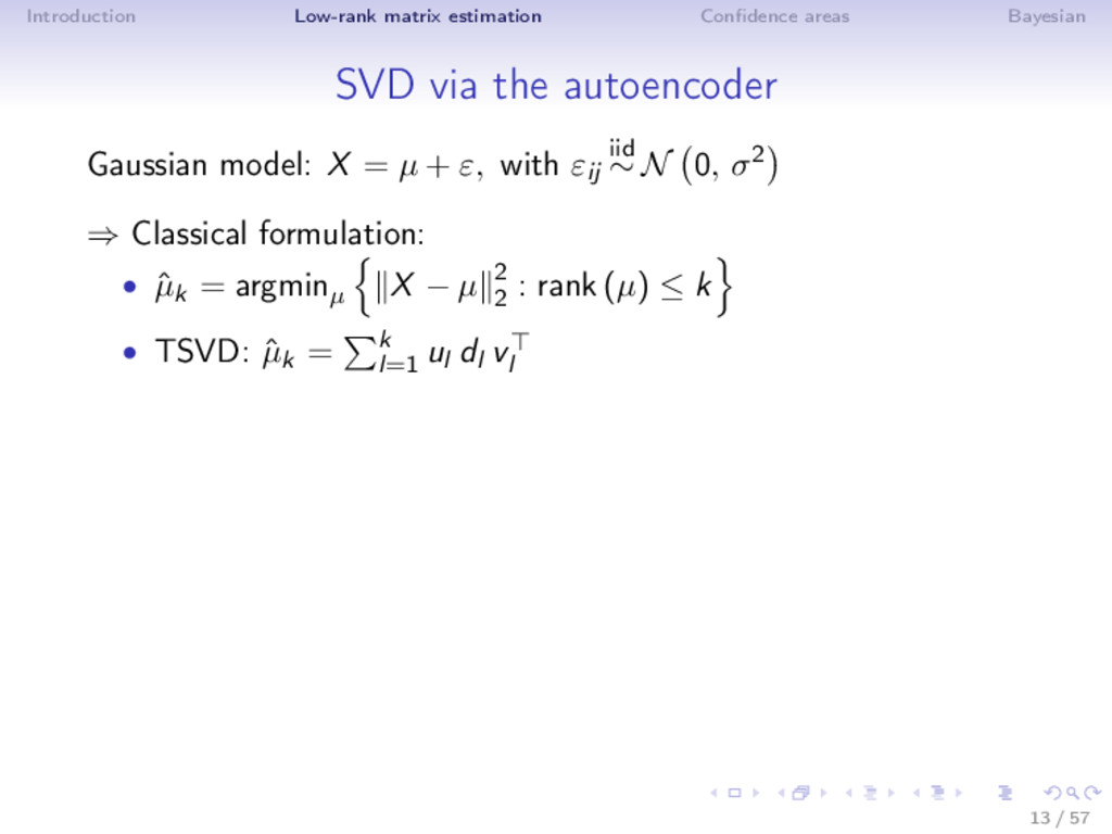
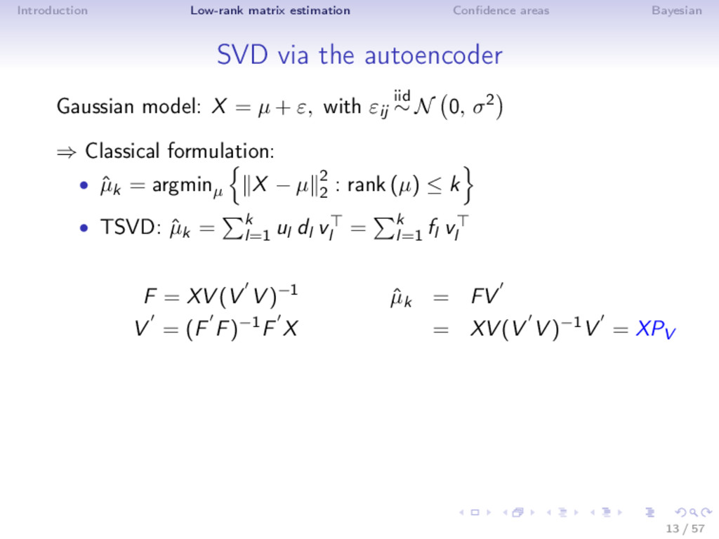
17. Introduction Low-rank matrix estimation Confidence areas Bayesian SVD via the autoencoder Gaussian model: X = µ + ε, with εij iid ∼ N 0, σ2 ⇒ Classical formulation: • ˆ µk = argminµ X − µ 2 2 : rank (µ) ≤ k • TSVD: ˆ µk = k l=1 ul dl v l = k l=1 fl v l F = XV (V V )−1 V = (F F)−1F X ˆ µk = FV = XV (V V )−1V = XPV 13 / 57
18. Introduction Low-rank matrix estimation Confidence areas Bayesian SVD via the autoencoder Gaussian model: X = µ + ε, with εij iid ∼ N 0, σ2 ⇒ Classical formulation: • ˆ µk = argminµ X − µ 2 2 : rank (µ) ≤ k • TSVD: ˆ µk = k l=1 ul dl v l = k l=1 fl v l F = XV (V V )−1 V = (F F)−1F X ˆ µk = FV = XV (V V )−1V = XPV ⇒ Another formulation: autoencoder (Boulard & Kamp, 1988) ˆ µk = XBk, where Bk = argminB X − XB 2 2 : rank (B) ≤ k 13 / 57
19. Introduction Low-rank matrix estimation Confidence areas Bayesian Parametric Bootstrap Model: X = µ + ε, with εij ∼ N 0, σ2 ⇒ Autoencoder: compress X ˆ µk = XBk, where Bk = argminB X − XB 2 2 : rank (B) ≤ k ⇒ Aim: recover µ ˆ µ∗ k = XB∗ k , B∗ k = argminB EX∼L(µ) µ − XB 2 2 : rank (B) ≤ k 14 / 57
20. Introduction Low-rank matrix estimation Confidence areas Bayesian Parametric Bootstrap Model: X = µ + ε, with εij ∼ N 0, σ2 ⇒ Autoencoder: compress X ˆ µk = XBk, where Bk = argminB X − XB 2 2 : rank (B) ≤ k ⇒ Aim: recover µ ˆ µ∗ k = XB∗ k , B∗ k = argminB EX∼L(µ) µ − XB 2 2 : rank (B) ≤ k ⇒ Parametric Bootstrap ˆ µboot k = XBk, Bk = argminB EX∼L(X) X − XB 2 2 : rank (B) ≤ k 14 / 57
21. Introduction Low-rank matrix estimation Confidence areas Bayesian Stable Autoencoder ⇒ Bootstrap = Feature noising ˆ µboot k = XBk, Bk = argminB EX∼L(X) X − XB 2 2 : rkB ≤ k Bk = argminB Eε X − (X + ε)B 2 2 : rkB ≤ k 15 / 57
22. Introduction Low-rank matrix estimation Confidence areas Bayesian Stable Autoencoder ⇒ Bootstrap = Feature noising ˆ µboot k = XBk, Bk = argminB EX∼L(X) X − XB 2 2 : rkB ≤ k Bk = argminB Eε X − (X + ε)B 2 2 : rkB ≤ k ⇒ Equivalent to a ridge autoencoder problem ˆ µ(k) λ = XBλ, Bλ = argminB X − XB 2 2 + λ B 2 2 : rkB ≤ k 15 / 57
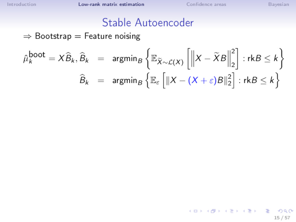
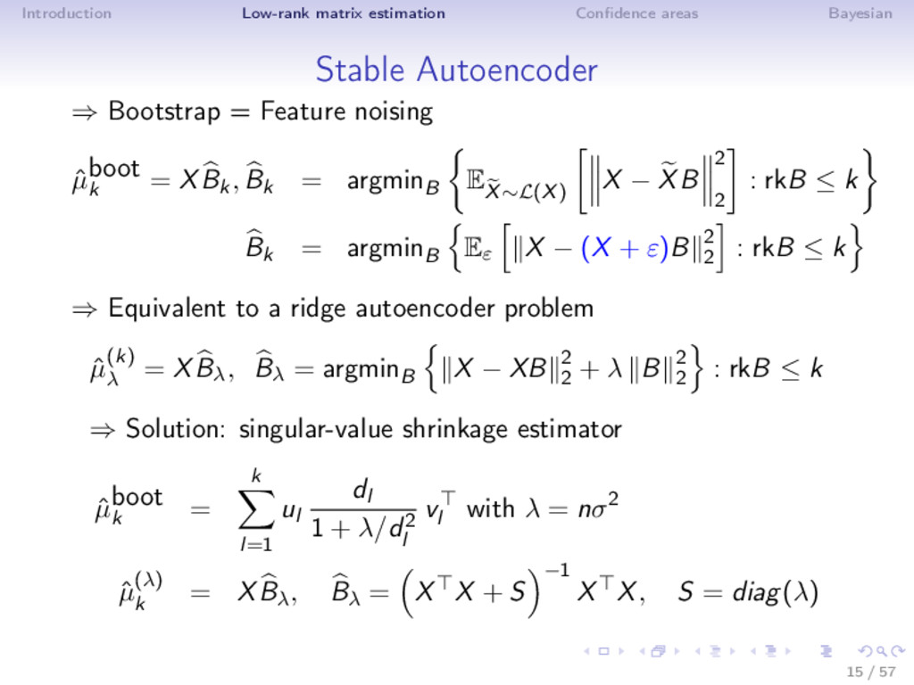
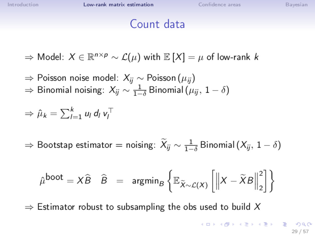
23. Introduction Low-rank matrix estimation Confidence areas Bayesian Stable Autoencoder ⇒ Bootstrap = Feature noising ˆ µboot k = XBk, Bk = argminB EX∼L(X) X − XB 2 2 : rkB ≤ k Bk = argminB Eε X − (X + ε)B 2 2 : rkB ≤ k ⇒ Equivalent to a ridge autoencoder problem ˆ µ(k) λ = XBλ, Bλ = argminB X − XB 2 2 + λ B 2 2 : rkB ≤ k ⇒ Solution: singular-value shrinkage estimator ˆ µboot k = k l=1 ul dl 1 + λ/d2 l vl with λ = nσ2 ˆ µ(λ) k = XBλ, Bλ = X X + S −1 X X, S = diag(λ) 15 / 57
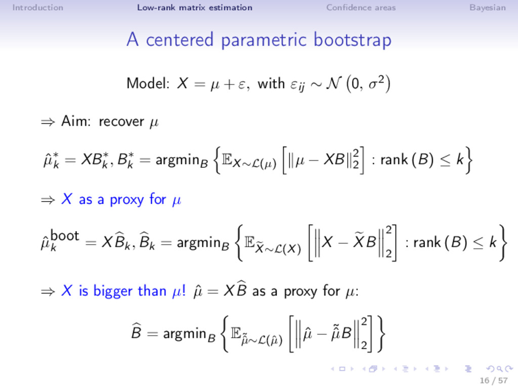
24. Introduction Low-rank matrix estimation Confidence areas Bayesian A centered parametric bootstrap Model: X = µ + ε, with εij ∼ N 0, σ2 ⇒ Aim: recover µ ˆ µ∗ k = XB∗ k , B∗ k = argminB EX∼L(µ) µ − XB 2 2 : rank (B) ≤ k ⇒ X as a proxy for µ ˆ µboot k = XBk, Bk = argminB EX∼L(X) X − XB 2 2 : rank (B) ≤ k ⇒ X is bigger than µ! ˆ µ = XB as a proxy for µ: B = argminB E˜ ˆ µ∼L(ˆ µ) ˆ µ − ˜ ˆ µB 2 2 16 / 57
25. Introduction Low-rank matrix estimation Confidence areas Bayesian Iterated Stable Autoencoder ˆ µISA = X ˆ B B = argminB E˜ ˆ µ∼L(ˆ µ) ˆ µ − ˜ ˆ µB 2 2 Iterative algorithm. Initialization: ˆ µ = X 1. ˆ µ = X ˆ B 2. B = argminB E˜ ˆ µ∼L(ˆ µ) ˆ µ − ˜ ˆ µB 2 2 1. ˆ µ = X ˆ B 2. ˆ B = (ˆ µ ˆ µ + S)−1 ˆ µ ˆ µ S = diag(nσ2) ⇒ ˆ µISA will be automatically of low rank!! 17 / 57
26. Introduction Low-rank matrix estimation Confidence areas Bayesian Simulations X200×500 = µ + ε k SNR Bootstrap TSVD Adaptive Asympt Soft SA ISA (σ, k) (σ) (k) (σ) - SURE (σ) (σ) - SURE MSE 10 4 0.004 0.004 0.004 0.004 0.004 0.008 100 4 0.037 0.036 0.037 0.037 0.037 0.045 10 2 0.017 0.017 0.017 0.017 0.017 0.033 100 2 0.142 0.143 0.152 0.142 0.146 0.156 10 1 0.067 0.067 0.072 0.067 0.067 0.116 100 1 0.511 0.775 0.733 0.448 0.600 0.448 10 0.5 0.277 0.251 0.321 0.253 0.250 0.353 100 0.5 1.600 1.000 3.164 0.852 0.961 0.852 Rank 10 4 10 11 10 65 100 4 100 103 100 193 10 2 10 11 10 63 100 2 100 114 100 181 10 1 10 11 10 59 100 1 29.6 154 64 154 10 0.5 10 15 10 51 100 0.5 0 87 15 86 18 / 57
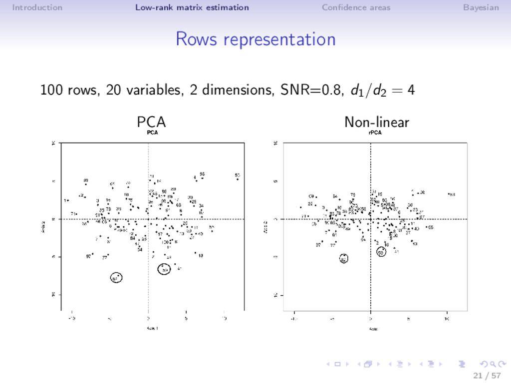
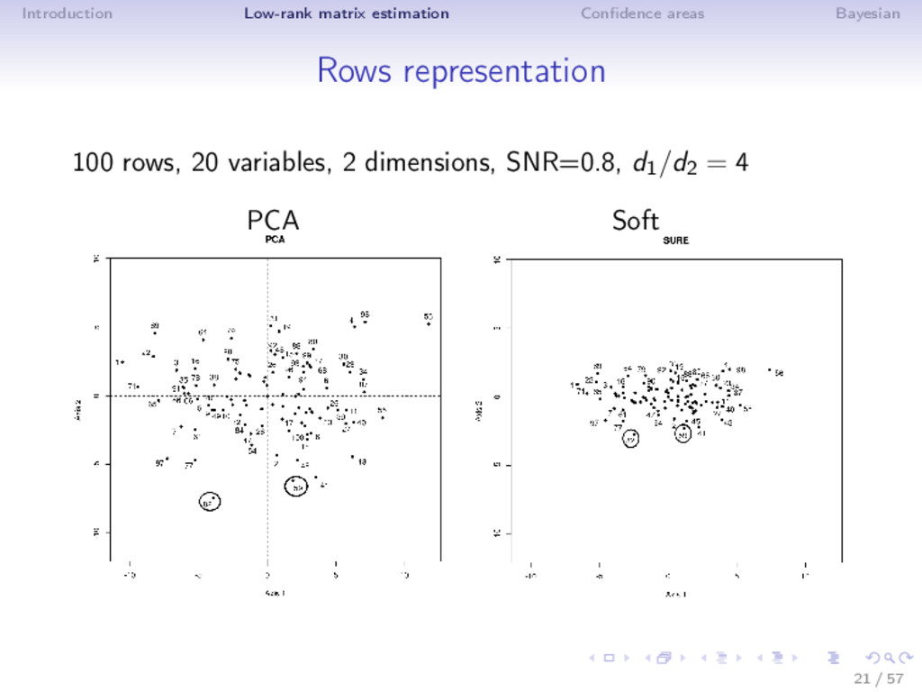
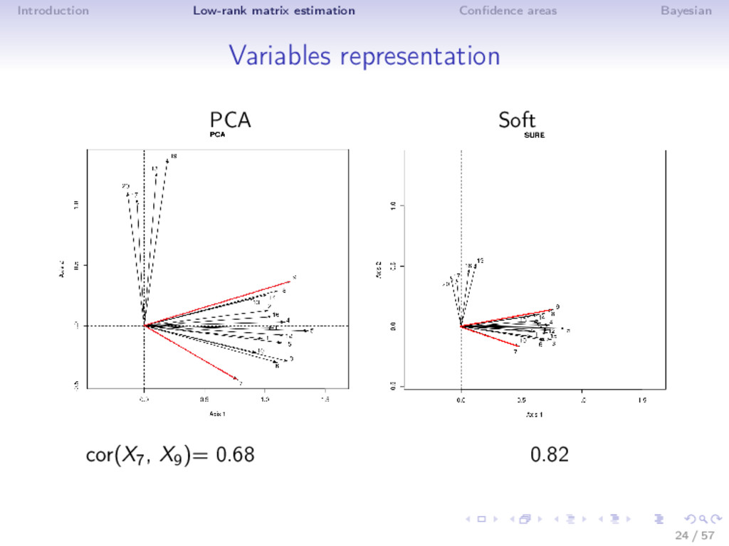
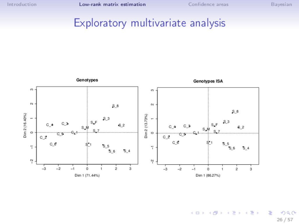
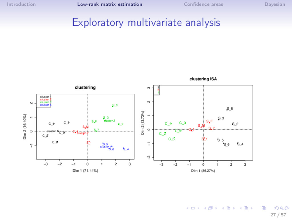
27. Introduction Low-rank matrix estimation Confidence areas Bayesian Simulation results ⇒ Different noise regime • low noise: truncated SVD • moderate noise: Asympt, SA, ISA (non-linear transformation) • high noise (SNR low, k large): Soft thresholding ⇒ Adaptive estimator is very flexible! (selection with SURE) ⇒ ISA performs well in MSE (even outside the Gaussian noise) and as a by-product estimates accurately the rank! Rq: not the usual behavior n > p: rows more perturbed than the columns; n < p: columns more perturbed; n = p 19 / 57
28. Introduction Low-rank matrix estimation Confidence areas Bayesian Rows representation 100 rows, 20 variables, 2 dimensions, SNR=0.8, d1/d2 = 4 True configuration PCA 20 / 57
29. Introduction Low-rank matrix estimation Confidence areas Bayesian Rows representation 100 rows, 20 variables, 2 dimensions, SNR=0.8, d1/d2 = 4 PCA Non-linear 21 / 57
30. Introduction Low-rank matrix estimation Confidence areas Bayesian Rows representation 100 rows, 20 variables, 2 dimensions, SNR=0.8, d1/d2 = 4 PCA Soft 21 / 57
31. Introduction Low-rank matrix estimation Confidence areas Bayesian Rows representation 100 rows, 20 variables, 2 dimensions, SNR=0.8, d1/d2 = 4 True configuration Non-linear ⇒ Improve the recovery of the inner-product matrix µµ 22 / 57
32. Introduction Low-rank matrix estimation Confidence areas Bayesian Variables representation True configuration PCA cor(X7, X9)= 1 0.68 23 / 57
33. Introduction Low-rank matrix estimation Confidence areas Bayesian Variables representation PCA Non-linear cor(X7, X9)= 0.68 0.81 24 / 57
34. Introduction Low-rank matrix estimation Confidence areas Bayesian Variables representation PCA Soft cor(X7, X9)= 0.68 0.82 24 / 57
35. Introduction Low-rank matrix estimation Confidence areas Bayesian Variables representation True configuration Non-linear cor(X7, X9)= 1 0.81 ⇒ Improve the recovery of the covariance matrix µ µ 25 / 57
36. Introduction Low-rank matrix estimation Confidence areas Bayesian Exploratory multivariate analysis −3 −2 −1 0 1 2 3 −2 −1 0 1 2 3 Genotypes Dim 1 (71.44%) Dim 2 (16.40%) C_1 C_2 C_3 C_4 C_5 C_6 S_1 S_2 S_3 S_4 S_5 S_6 S_7 S_8 S_F S_M −3 −2 −1 0 1 2 3 −2 −1 0 1 2 3 Genotypes ISA Dim 1 (86.27%) Dim 2 (13.73%) C_1 C_2 C_3 C_4 C_5 C_6 S_1 S_2 S_3 S_4 S_5 S_6 S_7 S_8 S_F S_M 26 / 57
37. Introduction Low-rank matrix estimation Confidence areas Bayesian Exploratory multivariate analysis −3 −2 −1 0 1 2 3 −1 0 1 2 clustering Dim 1 (71.44%) Dim 2 (16.40%) C_2 C_4 C_6 C_5 C_3 C_1 S_M S_1 S_F S_7 S_5 S_3 S_6 S_8 S_2 S_4 cluster 1 cluster 2 cluster 3 cluster 4 cluster 1 cluster 2 cluster 3 cluster 4 −3 −2 −1 0 1 2 3 −2 −1 0 1 2 3 clustering ISA Dim 1 (86.27%) Dim 2 (13.73%) C_1 C_2 C_3 C_4 C_5 C_6 S_1 S_2 S_3 S_4 S_5 S_6 S_7 S_8 S_F S_M 3 2 1 27 / 57
38. Introduction Low-rank matrix estimation Confidence areas Bayesian Outline 1. Plant-Breeding example 2. Regularized low rank matrix estimation • Singular-values shrinkage • Bootstrap approach (Josse & Wager, 2015...) • Bootstrap outside the Gaussian noise 3. Confidence areas for biplots: bootstrap/jaccknife 4. Bayesian treatment of SVD models 28 / 57
39. Introduction Low-rank matrix estimation Confidence areas Bayesian Count data ⇒ Model: X ∈ Rn×p ∼ L(µ) with E [X] = µ of low-rank k ⇒ Poisson noise model: Xij ∼ Poisson (µij ) ⇒ Binomial noising: Xij ∼ 1 1−δ Binomial (µij , 1 − δ) ⇒ ˆ µk = k l=1 ul dl v l ⇒ Bootstap estimator = noising: Xij ∼ 1 1−δ Binomial (Xij , 1 − δ) ˆ µboot = XB B = argminB EX∼L(X) X − XB 2 2 ⇒ Estimator robust to subsampling the obs used to build X 29 / 57
40. Introduction Low-rank matrix estimation Confidence areas Bayesian Bootstrap estimators ⇒ Feature noising = regularization B = argminB X − XB 2 2 + S 1 2 B 2 2 Sjj = n i=1 Var X∼L(X) Xij ˆ µ = X(X X + δ 1−δ S)−1X X, S diagonal with row-sums of X ⇒ New estimator ˆ µ that does not reduce to singular value shrinkage ⇒ ISA estimator - iterative algorithm 1. ˆ µ = X ˆ B 2. ˆ B = (ˆ µ ˆ µ + S)−1 ˆ µ ˆ µ 30 / 57
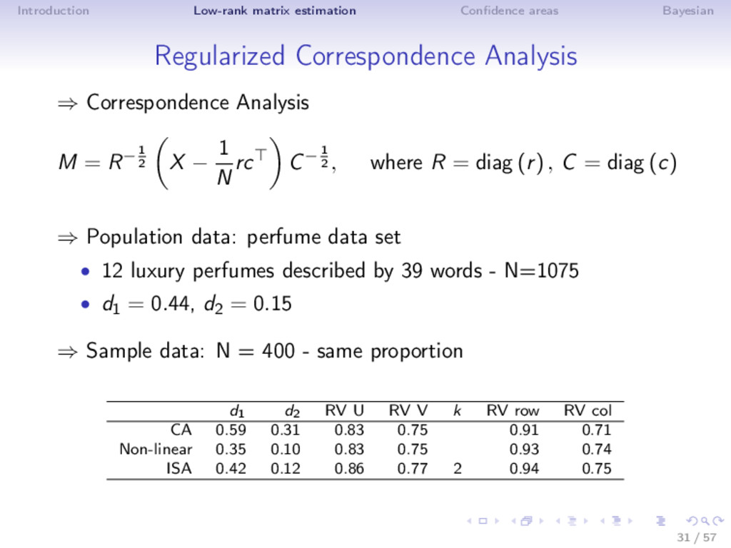
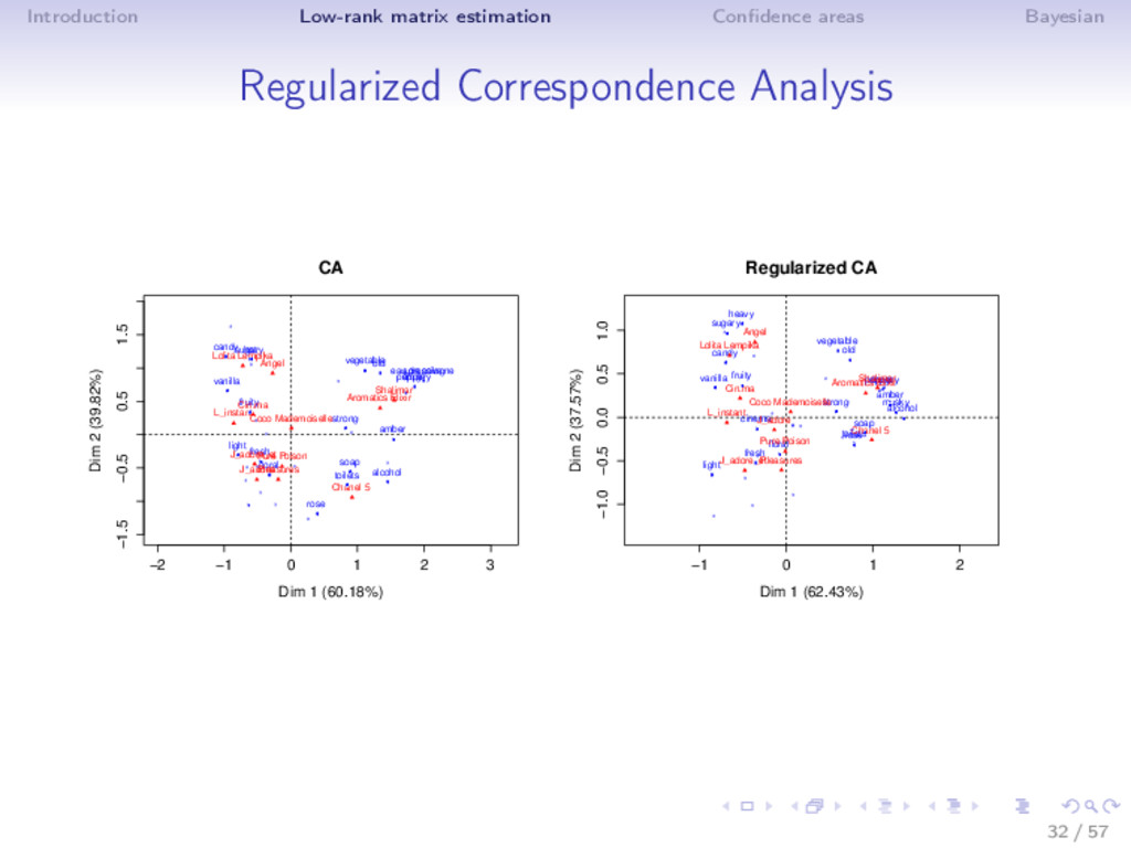
41. Introduction Low-rank matrix estimation Confidence areas Bayesian Regularized Correspondence Analysis ⇒ Correspondence Analysis M = R−1 2 X − 1 N rc C−1 2 , where R = diag (r) , C = diag (c) ⇒ Population data: perfume data set • 12 luxury perfumes described by 39 words - N=1075 • d1 = 0.44, d2 = 0.15 ⇒ Sample data: N = 400 - same proportion d1 d2 RV U RV V k RV row RV col CA 0.59 0.31 0.83 0.75 0.91 0.71 Non-linear 0.35 0.10 0.83 0.75 0.93 0.74 ISA 0.42 0.12 0.86 0.77 2 0.94 0.75 31 / 57
42. Introduction Low-rank matrix estimation Confidence areas Bayesian Regularized Correspondence Analysis −2 −1 0 1 2 3 −1.5 −0.5 0.5 1.5 CA Dim 1 (60.18%) Dim 2 (39.82%) floral fruity strong light sugary fresh soap vanilla old agressive toilets alcohol drugs hot peppery rose candy vegetable eau.de.cologne amber Angel Aromatics Elixir Chanel 5 Cin.ma Coco Mademoiselle J_adore J_adore_et L_instant Lolita Lempika Pleasures Pure Poison Shalimar −1 0 1 2 −1.0 −0.5 0.0 0.5 1.0 Regularized CA Dim 1 (62.43%) Dim 2 (37.57%) floral fruity strong cinema light sugary fresh soap vanilla old toilets alcohol heavy drugs peppery rose candy musky vegetable amber Angel Aromatics Elixir Chanel 5 Cin.ma Coco Mademoiselle J_adore J_adore_et L_instant Lolita Lempika Pleasures Pure Poison Shalimar 32 / 57
43. Introduction Low-rank matrix estimation Confidence areas Bayesian Regularized Correspondence Analysis q −1.0 −0.5 0.0 0.5 1.0 1.5 −1.0 −0.5 0.0 0.5 1.0 Factor map Dim 1 (65.41%) Dim 2 (34.59%) J_adore J_adore_et Pleasures cinema Pure Poison Coco Mademoiselle Lolita Lempika L_instant Angel Shalimar Chanel 5 Aromatics Elixir cluster 1 cluster 2 cluster 3 cluster 4 q q q q q q q q q q q q cluster 1 cluster 2 cluster 3 cluster 4 q −0.5 0.0 0.5 1.0 −1.0 −0.5 0.0 0.5 Factor map Dim 1 (77.13%) Dim 2 (22.87%) J_adore J_adore_et Pleasures cinema Pure Poison Coco Mademoiselle Lolita Lempika L_instant Angel Shalimar Chanel 5 Aromatics Elixir cluster 1 cluster 2 cluster 3 q q q q q q q q q q q q cluster 1 cluster 2 cluster 3 33 / 57
44. Introduction Low-rank matrix estimation Confidence areas Bayesian Outline 1. Plant-Breeding example 2. Regularized low rank matrix estimation • Singular-values shrinkage • Bootstrap approach 3. Confidence areas for biplots: bootstrap/jaccknife (Josse, Husson & Wager, 2014) 4. Bayesian treatment of SVD models 34 / 57
45. Introduction Low-rank matrix estimation Confidence areas Bayesian Inference in PCA −3 −2 −1 0 1 2 3 −2 −1 0 1 2 3 Genotypes Dim 1 (71.44%) Dim 2 (16.40%) C_1 C_2 C_3 C_4 C_5 C_6 S_1 S_2 S_3 S_4 S_5 S_6 S_7 S_8 S_F S_M 35 / 57
46. Introduction Low-rank matrix estimation Confidence areas Bayesian Inference in PCA −3 −2 −1 0 1 2 3 −3 −2 −1 0 1 2 Bootstrap Dim 1 (71.44%) Dim 2 (16.40%) C_1 C_2 C_3 C_4 C_5 C_6 S_1 S_2 S_3 S_4 S_5 S_6 S_7 S_8 S_F S_M 35 / 57
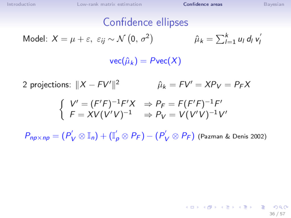
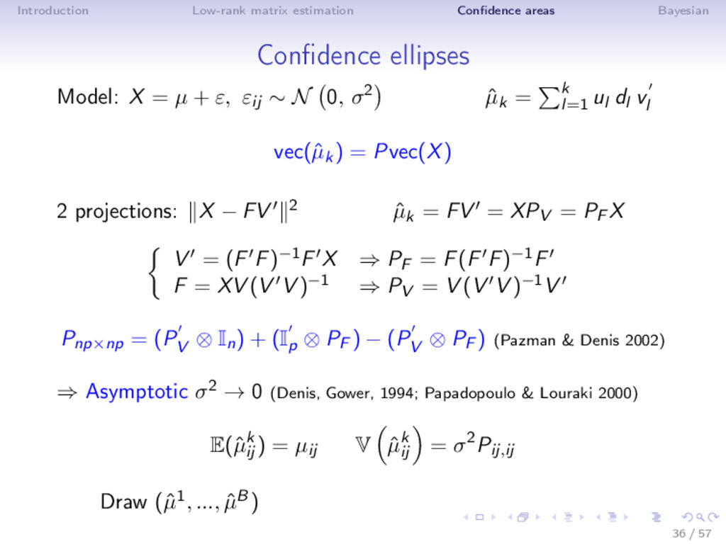
47. Introduction Low-rank matrix estimation Confidence areas Bayesian Confidence ellipses Model: X = µ + ε, εij ∼ N 0, σ2 ˆ µk = k l=1 ul dl v l vec(ˆ µk) = Pvec(X) 2 projections: X − FV 2 ˆ µk = FV = XPV = PF X V = (F F)−1F X ⇒ PF = F(F F)−1F F = XV (V V )−1 ⇒ PV = V (V V )−1V Pnp×np = (PV ⊗ In) + (Ip ⊗ PF ) − (PV ⊗ PF ) (Pazman & Denis 2002) 36 / 57
48. Introduction Low-rank matrix estimation Confidence areas Bayesian Confidence ellipses Model: X = µ + ε, εij ∼ N 0, σ2 ˆ µk = k l=1 ul dl v l vec(ˆ µk) = Pvec(X) 2 projections: X − FV 2 ˆ µk = FV = XPV = PF X V = (F F)−1F X ⇒ PF = F(F F)−1F F = XV (V V )−1 ⇒ PV = V (V V )−1V Pnp×np = (PV ⊗ In) + (Ip ⊗ PF ) − (PV ⊗ PF ) (Pazman & Denis 2002) ⇒ Asymptotic σ2 → 0 (Denis, Gower, 1994; Papadopoulo & Louraki 2000) E(ˆ µk ij ) = µij V ˆ µk ij = σ2Pij,ij Draw (ˆ µ1, ..., ˆ µB) 36 / 57
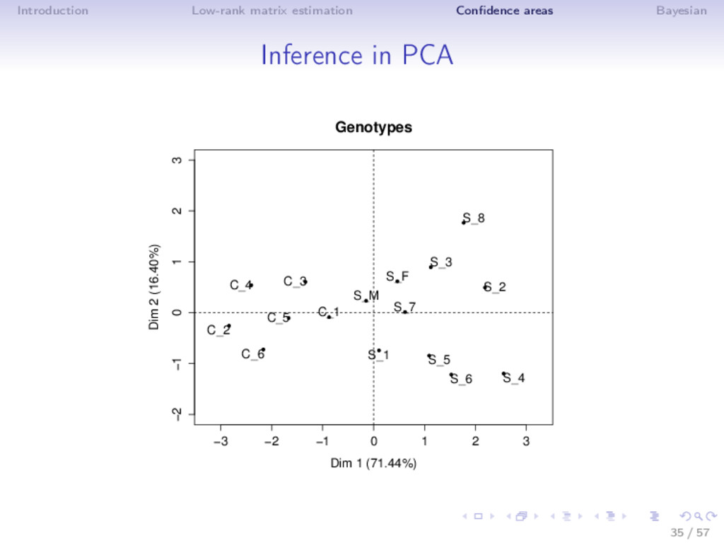
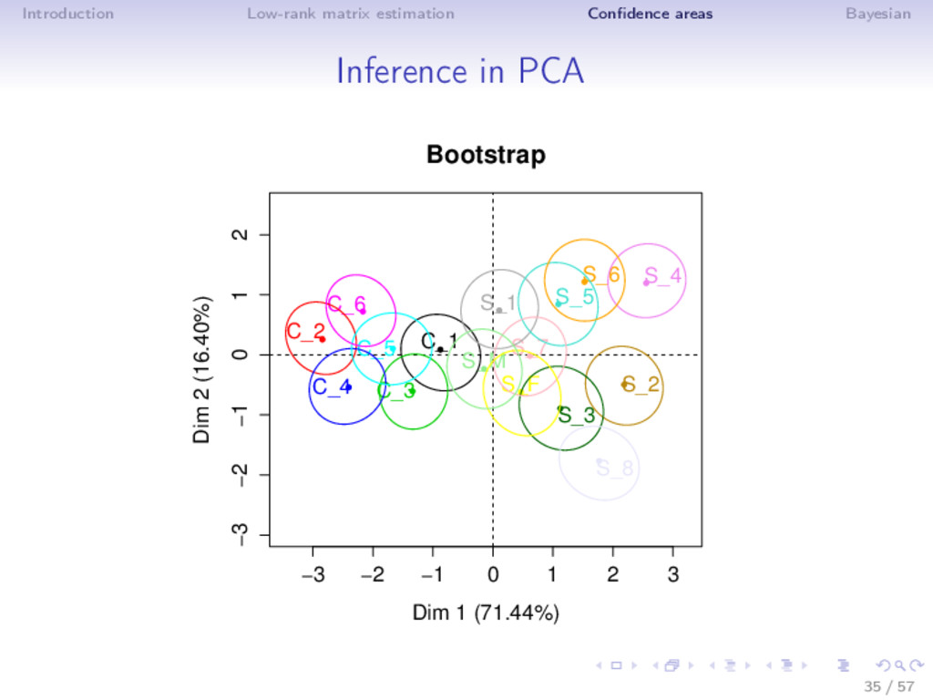
49. Introduction Low-rank matrix estimation Confidence areas Bayesian Confidence ellipses ⇒ Bootstrap ⇒ Rows bootstrap (Holmes, 1985, Timmerman et al, 2007) • random sample from a population - sampling variance • confidence areas around the position of the variables ⇒ Residuals bootstrap • full population data - X = µ + ε - noise fluctuation • confidence areas around the individuals and the variables 37 / 57
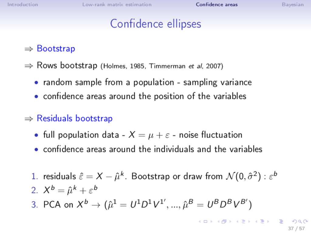
50. Introduction Low-rank matrix estimation Confidence areas Bayesian Confidence ellipses ⇒ Bootstrap ⇒ Rows bootstrap (Holmes, 1985, Timmerman et al, 2007) • random sample from a population - sampling variance • confidence areas around the position of the variables ⇒ Residuals bootstrap • full population data - X = µ + ε - noise fluctuation • confidence areas around the individuals and the variables 1. residuals ˆ ε = X − ˆ µk. Bootstrap or draw from N(0, ˆ σ2) : εb 2. Xb = ˆ µk + εb 3. PCA on Xb → (ˆ µ1 = U1D1V 1 , ..., ˆ µB = UBDBV B ) 37 / 57
51. Introduction Low-rank matrix estimation Confidence areas Bayesian Confidence ellipses ⇒ Jackknife 38 / 57
52. Introduction Low-rank matrix estimation Confidence areas Bayesian Confidence ellipses ⇒ Cell-wise Jackknife ˆ µ(k)(−ij) the estimator from the matrix without the cell (ij) ˆ µ(k)(ij) jackk = ˆ µk + √ np ˆ µ(k)(−ij) − ˆ µk Represent pseudo-values: (ˆ µ1, ..., ˆ µnp) Requires a method to deal with missing values - costly 38 / 57
53. Introduction Low-rank matrix estimation Confidence areas Bayesian Confidence ellipses ⇒ Cell-wise Jackknife ˆ µ(k)(−ij) the estimator from the matrix without the cell (ij) ˆ µ(k)(ij) jackk = ˆ µk + √ np ˆ µ(k)(−ij) − ˆ µk Represent pseudo-values: (ˆ µ1, ..., ˆ µnp) Requires a method to deal with missing values - costly ⇒ Approximate Jackknife (Craven & Wahba, 1979 lemma) In regression ˆ y = Py: ˆ y−i i − yi = ˆ yi −yi 1−Pi,i In PCA vec(ˆ µk) = Pvec(X) xij − ˆ µ(k)(−ij) ij xij − ˆ µk ij 1 − Pij,ij 38 / 57
54. Introduction Low-rank matrix estimation Confidence areas Bayesian Visualizing confidence areas ⇒ Spread of (ˆ µ1, ..., ˆ µB) gives the variability of PCA PCA Procrustes rotation PCA rotation 39 / 57
55. Introduction Low-rank matrix estimation Confidence areas Bayesian Simulations Model: X = µ + ε, εij ∼ N 0, σ2 • n/p: 100/20, 50/50 and 20/100 • k: 2, 4 - the ratio d1/d2: 4, 1 - SNR: 4, 1, 0.8 Coverage properties q −20 −10 0 10 20 30 −20 −10 0 10 20 Dim 1 (41.59%) Dim 2 (14.72%) q q q q q q q q q q q q q q q q q q q q ⇒ Different regimes: • High SNR - n large: Asymptotic ≈ Bootstrap • Small SNR: Jackknifes 40 / 57
56. Introduction Low-rank matrix estimation Confidence areas Bayesian Inference in PCA graphs −3 −2 −1 0 1 2 3 −3 −2 −1 0 1 2 Bootstrap Dim 1 (71.44%) Dim 2 (16.40%) C_1 C_2 C_3 C_4 C_5 C_6 S_1 S_2 S_3 S_4 S_5 S_6 S_7 S_8 S_F S_M −4 −2 0 2 4 6 −6 −4 −2 0 2 Jackknife Dim 1 (71.44%) Dim 2 (16.40%) C_1 C_2 C_3 C_4 C_5 C_6 S_1 S_2 S_3 S_4 S_5 S_6 S_7 S_8 S_F S_M 41 / 57
57. Introduction Low-rank matrix estimation Confidence areas Bayesian Inference in PCA graphs ⇒ Simulation based on the GE data (fitted rank 2: true) σ Asympt Bootstrap Jack Approx. Jack. 1 0.05 93.50 93.56 92.56 90.34 2 0.10 94.56 94.47 93.81 91.97 3 0.15 93.47 94.06 94.09 92.25 4 0.30 90.97 93.06 94.66 91.72 5 0.50 84.94 90.81 95.97 91.22 6 0.80 71.72 84.72 97.16 89.44 7 1.00 66.59 81.38 97.16 88.44 42 / 57
58. Introduction Low-rank matrix estimation Confidence areas Bayesian Confidences ellipses • k > 2 • Incorporating the uncertainty of k! Inference after model selection... • Variance of other estimators 43 / 57
59. Introduction Low-rank matrix estimation Confidence areas Bayesian Outline 1. Plant-Breeding example 2. Regularized low rank matrix estimation • Singular-values shrinkage • Bootstrap approach (Josse & Wager, 2015...) • Bootstrap outside the Gaussian noise 3. Confidence areas for biplots: bootstrap/jaccknife 4. Bayesian treatment of SVD models 44 / 57
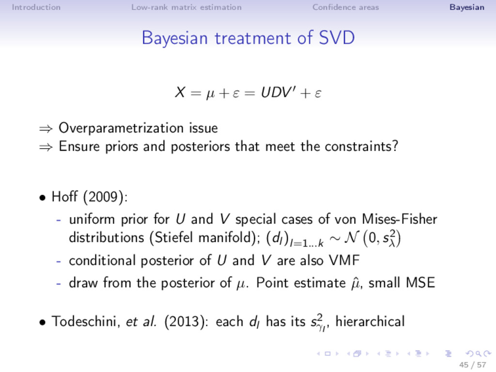
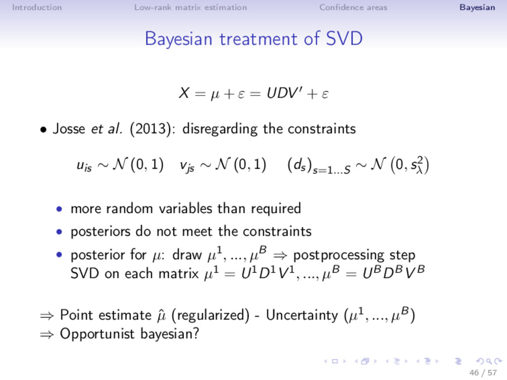
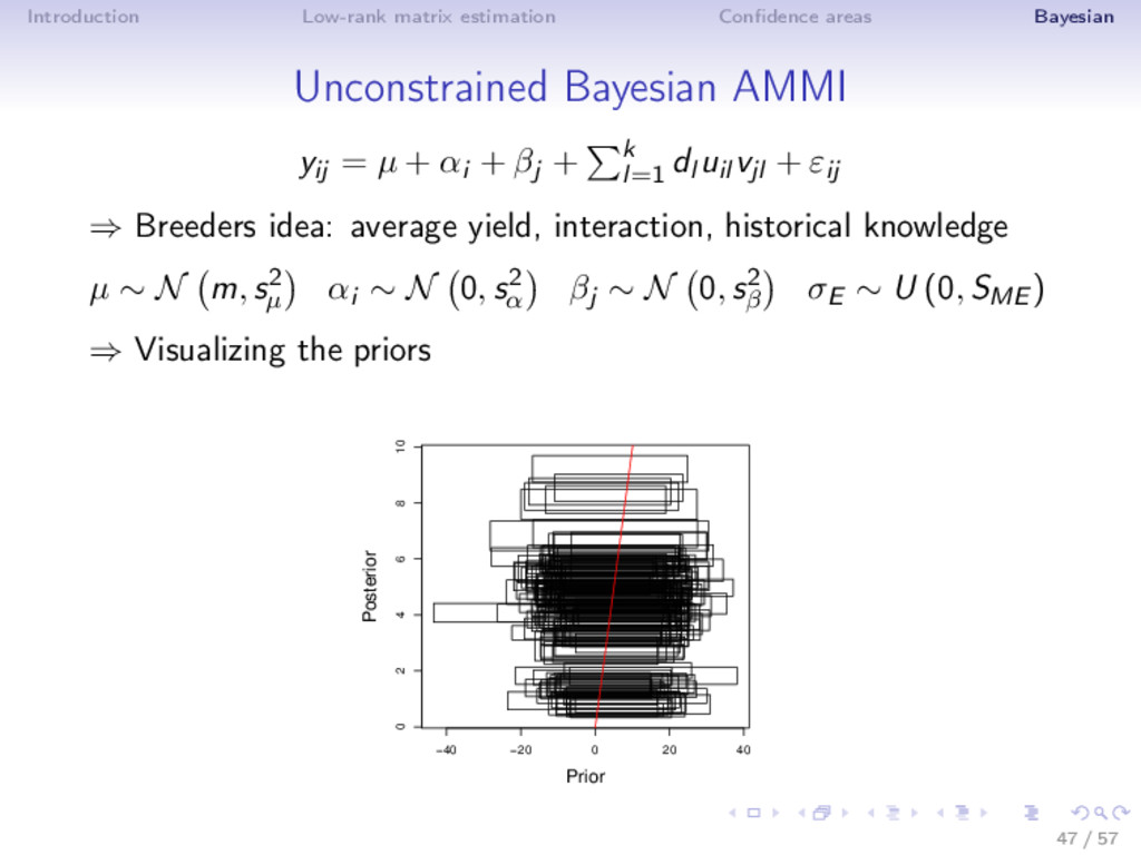
60. Introduction Low-rank matrix estimation Confidence areas Bayesian Bayesian treatment of SVD X = µ + ε = UDV + ε ⇒ Overparametrization issue ⇒ Ensure priors and posteriors that meet the constraints? • Hoff (2009): - uniform prior for U and V special cases of von Mises-Fisher distributions (Stiefel manifold); (dl )l=1...k ∼ N 0, s2 λ - conditional posterior of U and V are also VMF - draw from the posterior of µ. Point estimate ˆ µ, small MSE • Todeschini, et al. (2013): each dl has its s2 γl , hierarchical 45 / 57
61. Introduction Low-rank matrix estimation Confidence areas Bayesian Bayesian treatment of SVD X = µ + ε = UDV + ε • Josse et al. (2013): disregarding the constraints uis ∼ N (0, 1) vjs ∼ N (0, 1) (ds)s=1...S ∼ N 0, s2 λ • more random variables than required • posteriors do not meet the constraints • posterior for µ: draw µ1, ..., µB ⇒ postprocessing step SVD on each matrix µ1 = U1D1V 1, ..., µB = UBDBV B ⇒ Point estimate ˆ µ (regularized) - Uncertainty (µ1, ..., µB) ⇒ Opportunist bayesian? 46 / 57
62. Introduction Low-rank matrix estimation Confidence areas Bayesian Unconstrained Bayesian AMMI yij = µ + αi + βj + k l=1 dl uil vjl + εij ⇒ Breeders idea: average yield, interaction, historical knowledge µ ∼ N m, s2 µ αi ∼ N 0, s2 α βj ∼ N 0, s2 β σE ∼ U (0, SME ) ⇒ Visualizing the priors −40 −20 0 20 40 0 2 4 6 8 10 Prior Posterior 47 / 57
63. Introduction Low-rank matrix estimation Confidence areas Bayesian Unconstrained Bayesian AMMI 48 / 57
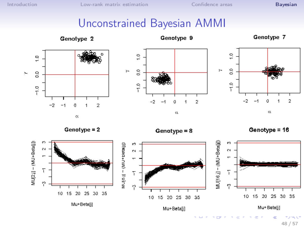
64. Introduction Low-rank matrix estimation Confidence areas Bayesian Unconstrained Bayesian AMMI ⇒ Easy to answer questions in a unique framework: best genotypes across environments, for one environment, stability, probability that a genotype produces less than a certain threshold? ⇒ To use for PCA graphs (shrinked biplot + ellipses) ⇒ Properties? Comparison? ⇒ Uncertainty on k... 49 / 57
65. Introduction Low-rank matrix estimation Confidence areas Bayesian Discussion ⇒ Low rank matrix estimation: point estimates/variability • Iterated Stable Autoencoder: good denoiser - automatic rank • ISA count data, networks - graphs (spectral clustering), latent semantic analysis • Bayesian ISA? • R package • Extension tensor: Hoff (2013): Bayesian Tucker • Missing values 50 / 57
66. Introduction Low-rank matrix estimation Confidence areas Bayesian 51 / 57
67. Introduction Low-rank matrix estimation Confidence areas Bayesian 52 / 57
68. Introduction Low-rank matrix estimation Confidence areas Bayesian Estimation of σ2 ⇒ Number of independent parameters ˆ σ2 = RSS ddl = n p l=k+1 dl np − p − nk − pk + k2 + k (Xn×p; Fn×k; Vp×k) ⇒ Trace of the PCA projection matrix 2 projection matrices: Xn×p − Fn×kV k×p 2 V = (F F)−1F X ⇒ PF = F(F F)−1F F = XV (V V )−1 ⇒ PV = V (V V )−1V ˆ µk = FV = XPV = PF X vec(ˆ µ) = Pvec(X) Pnp×np = (PV ⊗ In) + (Ip ⊗ PF ) − (PV ⊗ PF ) Pazman & Denis, 2002; Candes & Tao, 2009 53 / 57
69. Introduction Low-rank matrix estimation Confidence areas Bayesian Selecting the number of dimensions (Josse & Husson, 2012) ? ? ? ? ? ? ? ? ? ? ? ? ? ? ? ? ? ? ? ? ⇒ EM-CV (Bro et al. 2008) ⇒ MSEPS = 1 np n i=1 p j=1 (xij − ˆ µ−ij ij )2 ⇒ Computational costly In regression ˆ y = Py (Craven & Whaba, 1979): ˆ y−i i − yi = ˆ yi −yi 1−Pi,i vec(ˆ µk) = Pvec(X) P = (PV ⊗ In) + (Ip ⊗ PF ) − (PV ⊗ PF ) ACVk = 1 np i,j ˆ µij − xij 1 − Pij,ij 2 GCVk = 1 np × i,j (ˆ µij − xij )2 (1 − trP/np)2 54 / 57
70. Introduction Low-rank matrix estimation Confidence areas Bayesian Selecting the number of dimensions (Josse & Husson, 2012) ? ? ? ? ? ? ? ? ? ? ? ? ? ? ? ? ? ? ? ? ⇒ EM-CV (Bro et al. 2008) ⇒ MSEPS = 1 np n i=1 p j=1 (xij − ˆ µ−ij ij )2 ⇒ Computational costly In regression ˆ y = Py (Craven & Whaba, 1979): ˆ y−i i − yi = ˆ yi −yi 1−Pi,i vec(ˆ µk) = Pvec(X) P = (PV ⊗ In) + (Ip ⊗ PF ) − (PV ⊗ PF ) ACVk = 1 np i,j ˆ µij − xij 1 − Pij,ij 2 GCVk = 1 np × i,j (ˆ µij − xij )2 (1 − trP/np)2 54 / 57
71. Introduction Low-rank matrix estimation Confidence areas Bayesian Selecting the number of dimensions (Josse & Husson, 2012) ? ? ? ? ? ? ? ? ? ? ? ? ? ? ? ? ? ? ? ? ⇒ EM-CV (Bro et al. 2008) ⇒ MSEPS = 1 np n i=1 p j=1 (xij − ˆ µ−ij ij )2 ⇒ Computational costly In regression ˆ y = Py (Craven & Whaba, 1979): ˆ y−i i − yi = ˆ yi −yi 1−Pi,i vec(ˆ µk) = Pvec(X) P = (PV ⊗ In) + (Ip ⊗ PF ) − (PV ⊗ PF ) ACVk = 1 np i,j ˆ µij − xij 1 − Pij,ij 2 GCVk = 1 np × i,j (ˆ µij − xij )2 (1 − trP/np)2 54 / 57
72. Introduction Low-rank matrix estimation Confidence areas Bayesian Real data set • 27 chickens submitted to 4 nutritional statuses • 12664 gene expressions PCA rPCA 55 / 57
73. Introduction Low-rank matrix estimation Confidence areas Bayesian Real data set PCA rPCA Bi-clustering from rPCA better find the 4 nutritional statuses! 56 / 57
74. Introduction Low-rank matrix estimation Confidence areas Bayesian Random effect models: Probabilistic PCA ⇒ A specific factor analysis model (Roweis, 1998, Tipping & Bishop, 1999) xij = (Zn×kB p×k )ij + εij , zi ∼ N(0, Ik), εi ∼ N(0, σ2 Ip) • Conditional independence : xi |zi ∼ N(Bzi , σ2 Ip) • Distribution i.i.d: xi ∼ N(0, Σ = BB + σ2 Ip) • Max Lik.: ˆ σ2 = 1 p−k p l=k+1 λl ˆ B = V (D − σ2 Ik)1 2 ⇒ BLUP E(zi |xi ): ˆ Z = X ˆ B(ˆ B ˆ B + σ2 Ik)−1 ˆ µppca = ˆ Z ˆ B ˆ µ ppca ij = k l=1 dl − σ2 dl uil vjl ⇒ Bayesian SVD with a priori on U: Regularized PCA 57 / 57