Model Predictive Control for Uncertain Systems: Robust & Data-Driven Designs

Keynote talk at the Control Colloquium, Bosch Research, Renningen. Covers recent advances in robust and data-driven MPC for guaranteeing safety, stability, and performance under model uncertainty.

Transcript

1. Model predictive control for uncertain systems Robust & data-driven designs Johannes Köhler Imperial College London Bosch CR Colloquium Control Engineering - 5th October 2026 1
2. Control applications Cluttered [Köhler et al., 2025] Drone [Benders et al., 2025c] Racecars [Pabon et al., 2024] Robotic manipulators [Nubert et al., 2020, Wullt et al., 2026] Soft robots [Alora et al., 2023] 2
3. Challenges in control design 3
4. Challenges in control design How can we enforce safety-critical constraints for nonlinear systems? ⇒ Optimization-based design using predictive control 3
5. Challenges in control design How can we enforce safety-critical constraints for nonlinear systems? ⇒ Optimization-based design using predictive control How can we account for the uncertainty? ⇒ Robust design using contraction metrics 3
6. Challenges in control design How can we enforce safety-critical constraints for nonlinear systems? ⇒ Optimization-based design using predictive control How can we account for the uncertainty? ⇒ Robust design using contraction metrics How to characterize system dynamics and model uncertainty? ⇒ Data-driven designs and online adaptation/learning 3
7. Outline Model predictive control Robust design Data-driven design 4
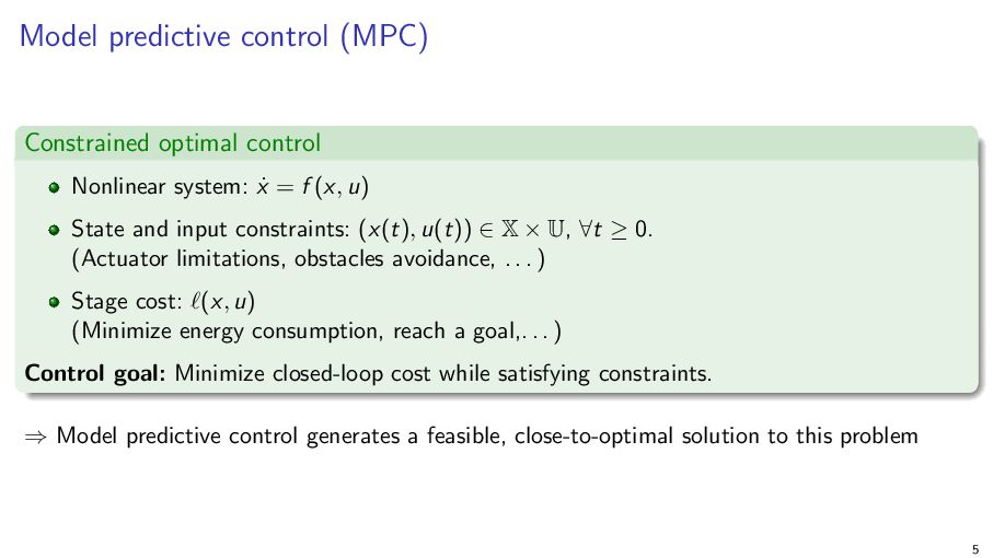
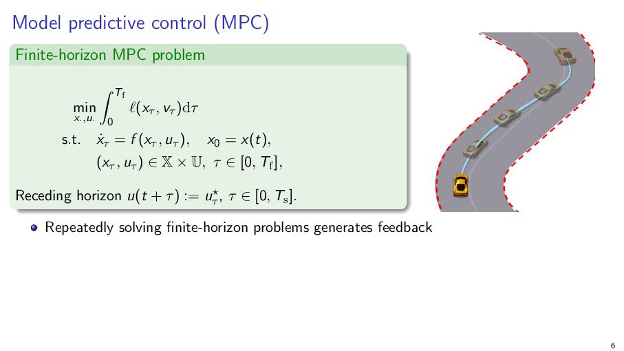
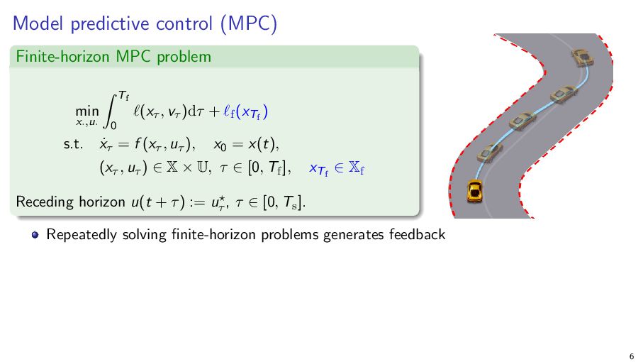
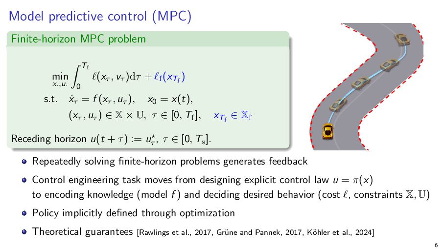
8. Model predictive control (MPC) Constrained optimal control Nonlinear system: ẋ = f (x, u) State and input constraints: (x(t), u(t)) ∈ X × U, ∀t ≥ 0. (Actuator limitations, obstacles avoidance, . . . ) Stage cost: ℓ(x, u) (Minimize energy consumption, reach a goal,. . . ) Control goal: Minimize closed-loop cost while satisfying constraints. ⇒ Model predictive control generates a feasible, close-to-optimal solution to this problem 5
9. Model predictive control (MPC) Finite-horizon MPC problem min x· ,u· Z Tf ℓ(xτ , vτ )dτ 0 s.t. ẋτ = f (xτ , uτ ), x0 = x(t), (xτ , uτ ) ∈ X × U, τ ∈ [0, Tf ], Receding horizon u(t + τ ) := uτ⋆ , τ ∈ [0, Ts ]. Repeatedly solving finite-horizon problems generates feedback 6
10. Model predictive control (MPC) Finite-horizon MPC problem min x· ,u· Z Tf 0 ℓ(xτ , vτ )dτ + ℓf (xTf ) s.t. ẋτ = f (xτ , uτ ), x0 = x(t), (xτ , uτ ) ∈ X × U, τ ∈ [0, Tf ], xTf ∈ Xf Receding horizon u(t + τ ) := uτ⋆ , τ ∈ [0, Ts ]. Repeatedly solving finite-horizon problems generates feedback 6
11. Model predictive control (MPC) Finite-horizon MPC problem min x· ,u· Z Tf 0 ℓ(xτ , vτ )dτ + ℓf (xTf ) s.t. ẋτ = f (xτ , uτ ), x0 = x(t), (xτ , uτ ) ∈ X × U, τ ∈ [0, Tf ], xTf ∈ Xf Receding horizon u(t + τ ) := uτ⋆ , τ ∈ [0, Ts ]. Repeatedly solving finite-horizon problems generates feedback Control engineering task moves from designing explicit control law u = π(x) to encoding knowledge (model f ) and deciding desired behavior (cost ℓ, constraints X, U) Policy implicitly defined through optimization Theoretical guarantees [Rawlings et al., 2017, Grüne and Pannek, 2017, Köhler et al., 2024] 6
12. MPC in practice Solving MPC online can be challenging in fast applications 7
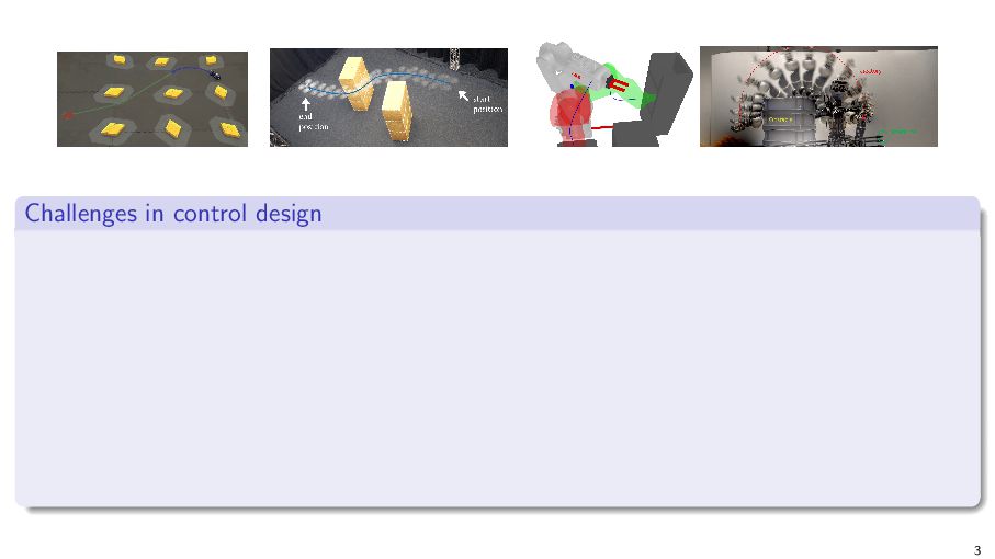
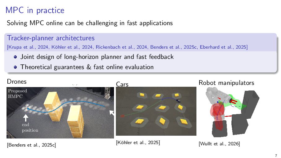
13. MPC in practice Solving MPC online can be challenging in fast applications Baseline SMPC Tracker-planner architectures [Krupa et al., 2024, Köhler et al., 2024, Rickenbach et al., 2024, Benders et al., 2025c, Eberhard et al., 2025] start position Joint design of long-horizon planner and fast feedback Theoretical guarantees & fast online evaluation end obstacles position Drones (a) Cars Robot manipulators Proposed HMPC start position end position [Benders et al., 2025c] (b) [Köhler et al., 2025] [Wullt et al., 2026] 7
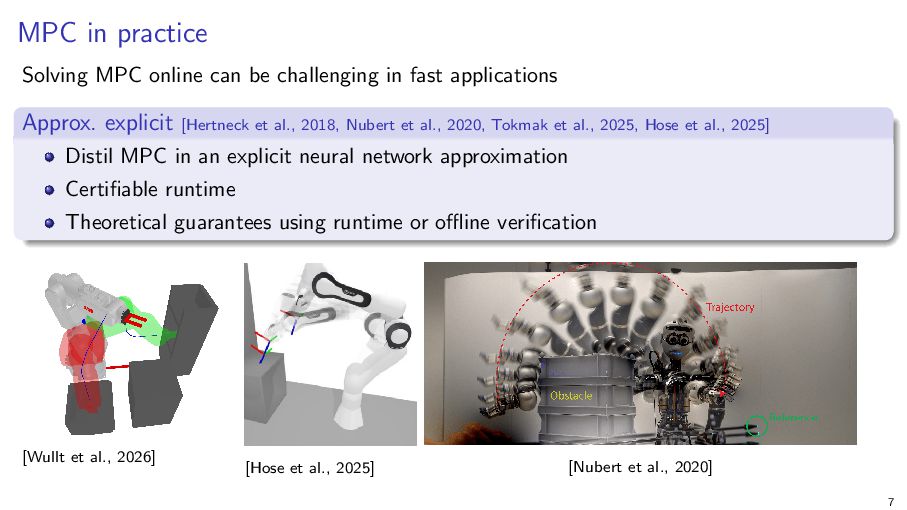
14. MPC in practice Solving MPC online can be challenging in fast applications Approx. explicit [Hertneck et al., 2018, Nubert et al., 2020, Tokmak et al., 2025, Hose et al., 2025] Distil MPC in an explicit neural network approximation Certifiable runtime Theoretical guarantees using runtime or offline verification [Wullt et al., 2026] [Hose et al., 2025] [Nubert et al., 2020] 7
15. MPC in practice Solving MPC online can be challenging in fast applications Tracker-planner architectures and explicit approximations can alleviate this issue. However, practical challenges go beyond computational speed. Problem MPC may fail if experiment deviates from model. . . ⇒ This talk focuses on model uncertainty. 7
16. Outline Model predictive control Robust design Data-driven design 8
17. Robust MPC design Robust control design Given a model with a known bound on the model mismatch. Design a controller that ensures satisfaction of safety-critical constraints x(t) ∈ X. 9
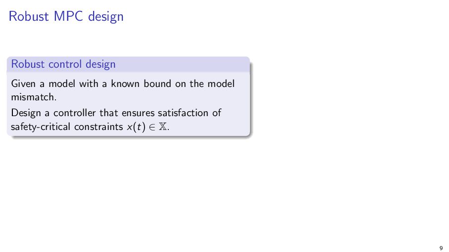
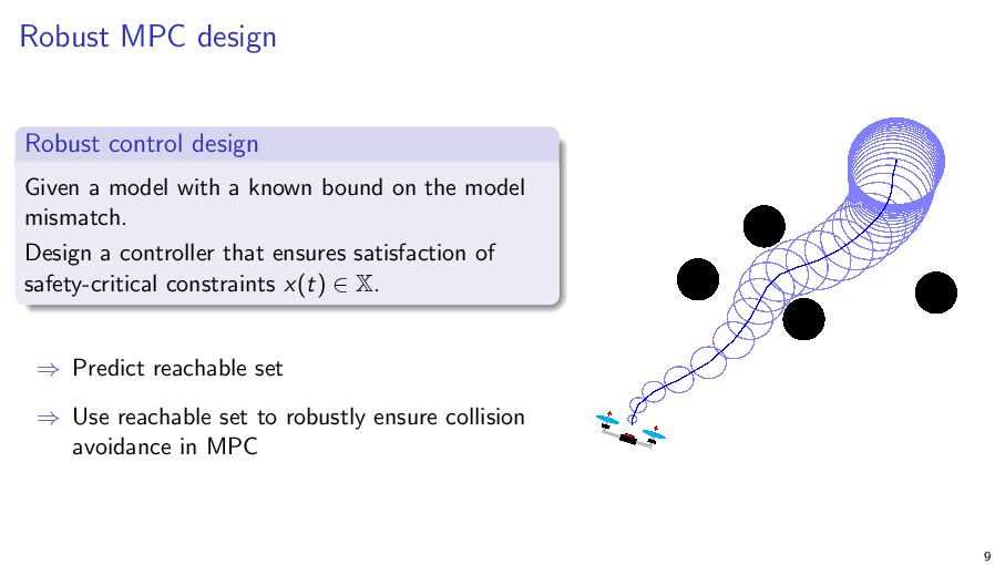
18. Robust MPC design Robust control design Given a model with a known bound on the model mismatch. Design a controller that ensures satisfaction of safety-critical constraints x(t) ∈ X. ⇒ Predict reachable set ⇒ Use reachable set to robustly ensure collision avoidance in MPC 9
19. Tube MPC [Köhler et al., 2021, Sasfi et al., 2023] Uncertain dynamics ẋ = fw (x, u, d), d ∈ D Nominal prediction: ż = f (z, v ) Feedback: u = κ(x, z, v ) Parametrised tube: R(t) = {x| Vδ (x, z(t)) ≤ δ(t)} Tube design Design feedback κ Choose ”distance measure”Vδ ; Find dynamics δ̇ = fδ (z, v , δ) Plots from [Zhao et al., 2022, Sasfi et al., 2023] ⇒ We address these steps with contraction metrics. 10
20. What are contraction metrics? Incremental exponential stability ∥x(t) − z(t)∥ ≤ Ce −ρt ∥x(0) − z(0)∥, ∀t ≥ 0, ẋ = f (x, u), ż = f (z, u), C ≥ 1, ρ > 0 Stability between trajectories ⇒ Natural tool for reachability analysis 11
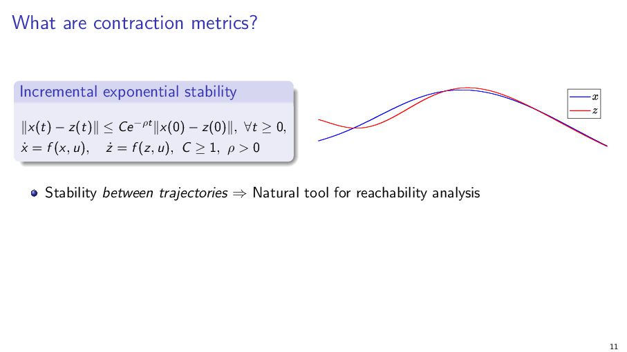
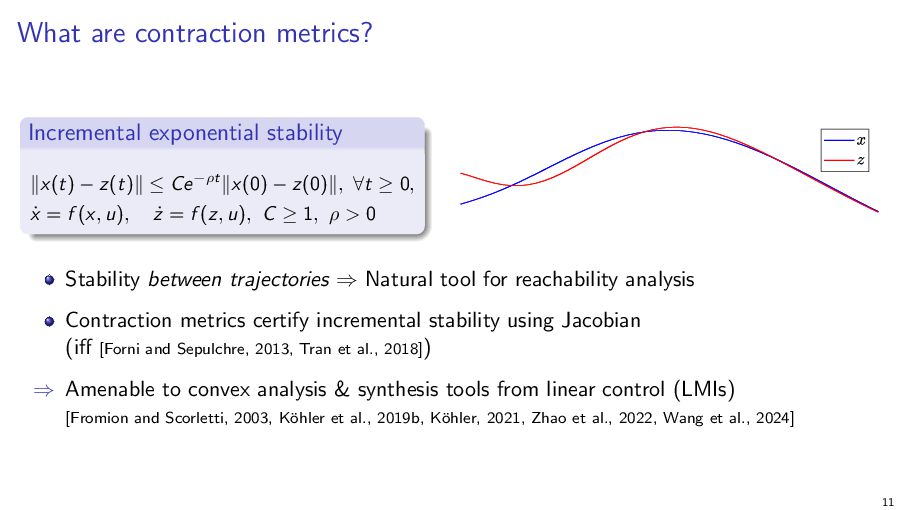
21. What are contraction metrics? Incremental exponential stability ∥x(t) − z(t)∥ ≤ Ce −ρt ∥x(0) − z(0)∥, ∀t ≥ 0, ẋ = f (x, u), ż = f (z, u), C ≥ 1, ρ > 0 Stability between trajectories ⇒ Natural tool for reachability analysis Contraction metrics certify incremental stability using Jacobian (iff [Forni and Sepulchre, 2013, Tran et al., 2018]) ⇒ Amenable to convex analysis & synthesis tools from linear control (LMIs) [Fromion and Scorletti, 2003, Köhler et al., 2019b, Köhler, 2021, Zhao et al., 2022, Wang et al., 2024] 11
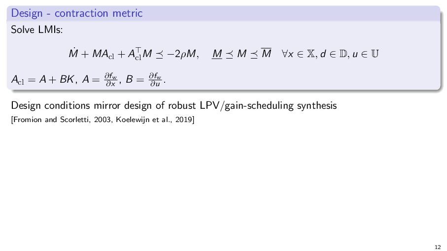
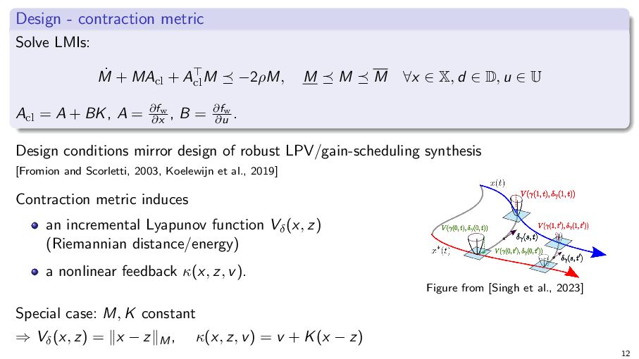
22. Design - contraction metric Solve LMIs: Ṁ + MAcl + A⊤ cl M ⪯ −2ρM, M⪯M⪯M ∀x ∈ X, d ∈ D, u ∈ U ∂fw w Acl = A + BK , A = ∂f ∂x , B = ∂u . Design conditions mirror design of robust LPV/gain-scheduling synthesis [Fromion and Scorletti, 2003, Koelewijn et al., 2019] 12
23. Design - contraction metric Solve LMIs: Ṁ + MAcl + A⊤ cl M ⪯ −2ρM, M⪯M⪯M ∀x ∈ X, d ∈ D, u ∈ U ∂fw w Acl = A + BK , A = ∂f ∂x , B = ∂u . Design conditions mirror design of robust LPV/gain-scheduling synthesis [Fromion and Scorletti, 2003, Koelewijn et al., 2019] Contraction metric induces an incremental Lyapunov function Vδ (x, z) (Riemannian distance/energy) a nonlinear feedback κ(x, z, v ). Figure from [Singh et al., 2023] Special case: M, K constant ⇒ Vδ (x, z) = ∥x − z∥M , κ(x, z, v ) = v + K (x − z) 12
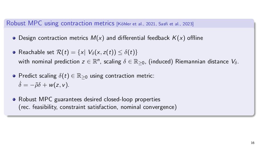
24. Incremental input-to-state stability [Sasfi et al., 2023] d Vδ (x, z) ≤ −ρ̃Vδ (x, z) + max ∥E (z, v )d∥M(z) d∈D dt | {z } w (z,v ) ẋ = f (x, u) + E (x, u)d, ż = f (z, v ), u = κ(x, z, v ), d ∈ D. Bound error based on disturbance d and contraction ρ̃ > 0 Uncertainty bound w (z, v ): worst-case model-mismatch for different state/input 13
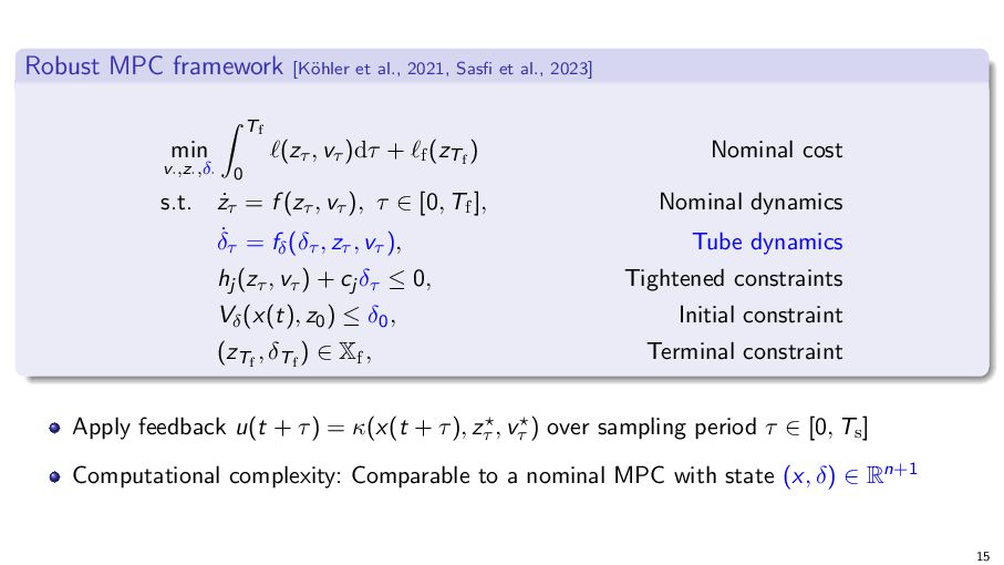
25. Robust reachability using contraction metrics [Sasfi et al., 2023] Consider Nominal dynamics: ż(t) = f (z(t), v (t)) Tube prediction: δ̇(t) = −ρ̃δ(t) + w (z(t), v (t)) Tightened constraints: Initial condition: hj (z(t), v (t)) + cj δ(t) ≤ 0, j = 1, . . . , r Vδ (x0 , z0 ) ≤ δ0 , Then, for all t ≥ 0, d(t) ∈ D: Predict robust reachable set: Vδ (x(t), z(t)) ≤ δ(t) Robust constraint satisfaction: (x(t), u(t)) ∈ X × U Tube scaling δ depends on the nominal trajectory z, v ⇒ if we operate the system in an area with more model error, we get a larger tube δ. 14
26. Robust MPC framework [Köhler et al., 2021, Sasfi et al., 2023] Z Tf ℓ(zτ , vτ )dτ + ℓf (zTf ) Nominal cost s.t. żτ = f (zτ , vτ ), τ ∈ [0, Tf ], Nominal dynamics δ̇τ = fδ (δτ , zτ , vτ ), Tube dynamics min v· ,z· ,δ· 0 hj (zτ , vτ ) + cj δτ ≤ 0, Tightened constraints Vδ (x(t), z0 ) ≤ δ0 , Initial constraint (zTf , δTf ) ∈ Xf , Terminal constraint Apply feedback u(t + τ ) = κ(x(t + τ ), zτ⋆ , vτ⋆ ) over sampling period τ ∈ [0, Ts ] Computational complexity: Comparable to a nominal MPC with state (x, δ) ∈ Rn+1 15
27. Robust MPC using contraction metrics [Köhler et al., 2021, Sasfi et al., 2023] Design contraction metrics M(x) and differential feedback K (x) offline Reachable set R(t) = {x| Vδ (x, z(t)) ≤ δ(t)} with nominal prediction z ∈ Rn , scaling δ ∈ R≥0 , (induced) Riemannian distance Vδ . Predict scaling δ(t) ∈ R≥0 using contraction metric: δ̇ = −ρ̃δ + w (z, v ). Robust MPC guarantees desired closed-loop properties (rec. feasibility, constraint satisfaction, nominal convergence) 16
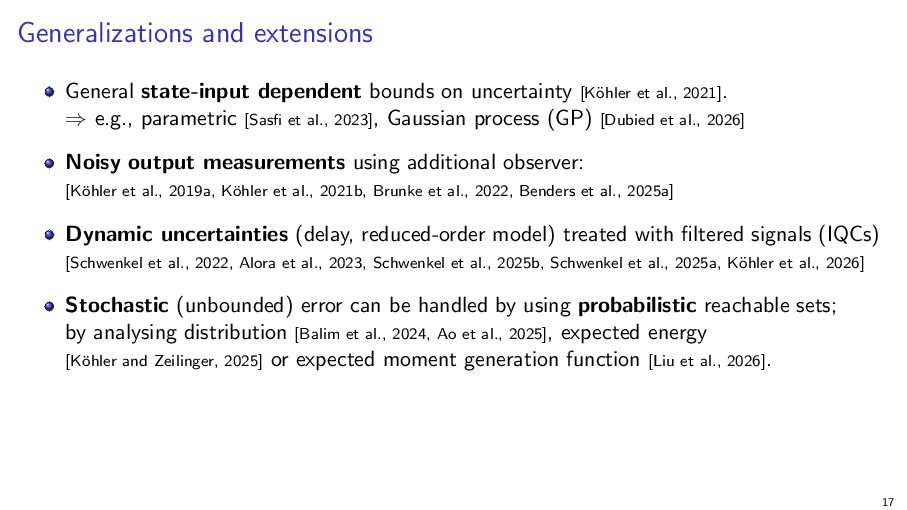
28. Generalizations and extensions General state-input dependent bounds on uncertainty [Köhler et al., 2021]. ⇒ e.g., parametric [Sasfi et al., 2023], Gaussian process (GP) [Dubied et al., 2026] Noisy output measurements using additional observer: [Köhler et al., 2019a, Köhler et al., 2021b, Brunke et al., 2022, Benders et al., 2025a] Dynamic uncertainties (delay, reduced-order model) treated with filtered signals (IQCs) [Schwenkel et al., 2022, Alora et al., 2023, Schwenkel et al., 2025b, Schwenkel et al., 2025a, Köhler et al., 2026] Stochastic (unbounded) error can be handled by using probabilistic reachable sets; by analysing distribution [Balim et al., 2024, Ao et al., 2025], expected energy [Köhler and Zeilinger, 2025] or expected moment generation function [Liu et al., 2026]. 17
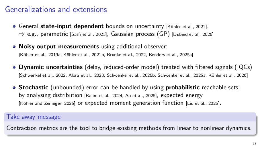
29. Generalizations and extensions General state-input dependent bounds on uncertainty [Köhler et al., 2021]. ⇒ e.g., parametric [Sasfi et al., 2023], Gaussian process (GP) [Dubied et al., 2026] Noisy output measurements using additional observer: [Köhler et al., 2019a, Köhler et al., 2021b, Brunke et al., 2022, Benders et al., 2025a] Dynamic uncertainties (delay, reduced-order model) treated with filtered signals (IQCs) [Schwenkel et al., 2022, Alora et al., 2023, Schwenkel et al., 2025b, Schwenkel et al., 2025a, Köhler et al., 2026] Stochastic (unbounded) error can be handled by using probabilistic reachable sets; by analysing distribution [Balim et al., 2024, Ao et al., 2025], expected energy [Köhler and Zeilinger, 2025] or expected moment generation function [Liu et al., 2026]. Take away message Contraction metrics are the tool to bridge existing methods from linear to nonlinear dynamics. 17
30. Numerical results Quadrotor - robust design [Sasfi et al., 2023] Model-mismatch depends on thrust/angle Offline design: 20 minutes Online optimization: 4-times slower than nominal Optimized trajectory: Slows down near obstacles; reduces uncertainty growth; squeezes through gap between obstacles 18
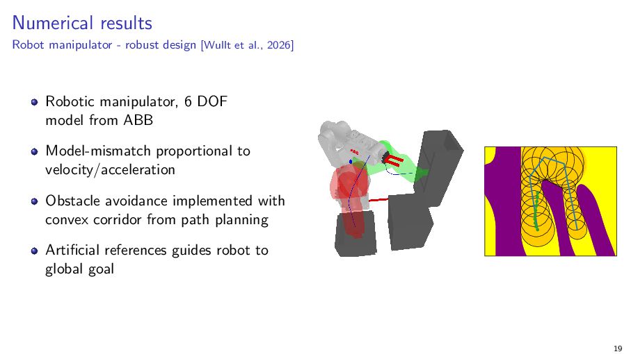
31. Numerical results Robot manipulator - robust design [Wullt et al., 2026] Robotic manipulator, 6 DOF model from ABB Model-mismatch proportional to velocity/acceleration Obstacle avoidance implemented with convex corridor from path planning Artificial references guides robot to global goal 19
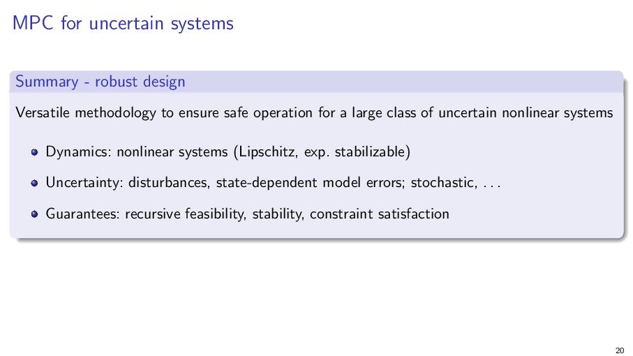
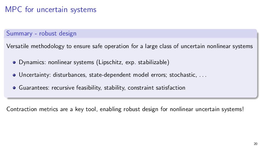
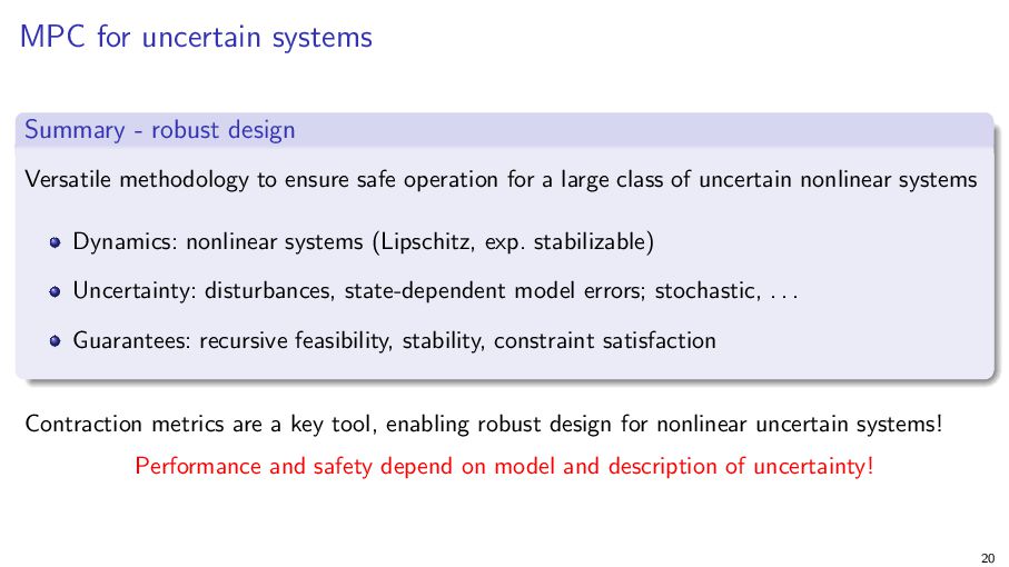
32. MPC for uncertain systems Summary - robust design Versatile methodology to ensure safe operation for a large class of uncertain nonlinear systems Dynamics: nonlinear systems (Lipschitz, exp. stabilizable) Uncertainty: disturbances, state-dependent model errors; stochastic, . . . Guarantees: recursive feasibility, stability, constraint satisfaction 20
33. MPC for uncertain systems Summary - robust design Versatile methodology to ensure safe operation for a large class of uncertain nonlinear systems Dynamics: nonlinear systems (Lipschitz, exp. stabilizable) Uncertainty: disturbances, state-dependent model errors; stochastic, . . . Guarantees: recursive feasibility, stability, constraint satisfaction Contraction metrics are a key tool, enabling robust design for nonlinear uncertain systems! 20
34. MPC for uncertain systems Summary - robust design Versatile methodology to ensure safe operation for a large class of uncertain nonlinear systems Dynamics: nonlinear systems (Lipschitz, exp. stabilizable) Uncertainty: disturbances, state-dependent model errors; stochastic, . . . Guarantees: recursive feasibility, stability, constraint satisfaction Contraction metrics are a key tool, enabling robust design for nonlinear uncertain systems! Performance and safety depend on model and description of uncertainty! 20
35. Outline Model predictive control Robust design Data-driven design 21
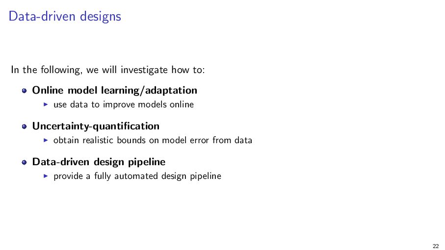
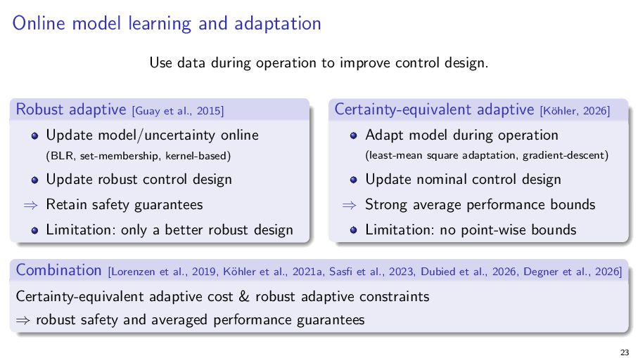
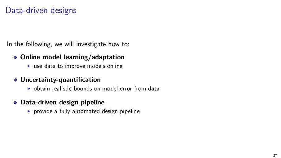
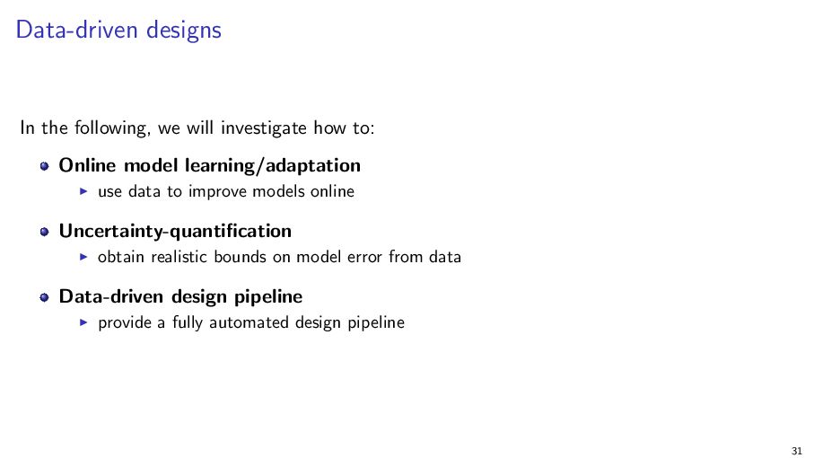
36. Data-driven designs In the following, we will investigate how to: Online model learning/adaptation ▶ use data to improve models online Uncertainty-quantification ▶ obtain realistic bounds on model error from data Data-driven design pipeline ▶ provide a fully automated design pipeline 22
37. Online model learning and adaptation Use data during operation to improve control design. 23
38. Online model learning and adaptation Use data during operation to improve control design. Robust adaptive [Guay et al., 2015] Update model/uncertainty online (BLR, set-membership, kernel-based) Update robust control design ⇒ Retain safety guarantees Limitation: only a better robust design 23
39. Online model learning and adaptation Use data during operation to improve control design. Robust adaptive [Guay et al., 2015] Certainty-equivalent adaptive [Köhler, 2026] Update model/uncertainty online Adapt model during operation (BLR, set-membership, kernel-based) (least-mean square adaptation, gradient-descent) Update robust control design Update nominal control design ⇒ Retain safety guarantees Limitation: only a better robust design ⇒ Strong average performance bounds Limitation: no point-wise bounds 23
40. Online model learning and adaptation Use data during operation to improve control design. Robust adaptive [Guay et al., 2015] Certainty-equivalent adaptive [Köhler, 2026] Update model/uncertainty online Adapt model during operation (BLR, set-membership, kernel-based) (least-mean square adaptation, gradient-descent) Update robust control design Update nominal control design ⇒ Retain safety guarantees Limitation: only a better robust design ⇒ Strong average performance bounds Limitation: no point-wise bounds Combination [Lorenzen et al., 2019, Köhler et al., 2021a, Sasfi et al., 2023, Dubied et al., 2026, Degner et al., 2026] Certainty-equivalent adaptive cost & robust adaptive constraints ⇒ robust safety and averaged performance guarantees 23
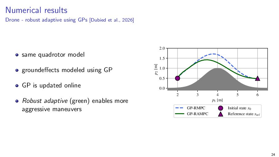
41. Numerical results Drone - robust adaptive using GPs [Dubied et al., 2026] 2.0 same quadrotor model p2 [m] groundeffects modeled using GP 1.5 1.0 0.5 GP is updated online 0.0 2 Robust adaptive (green) enables more aggressive maneuvers 3 GP-RMPC GP-RAMPC 4 p1 [m] 5 6 Initial state x0 Reference state xref 24
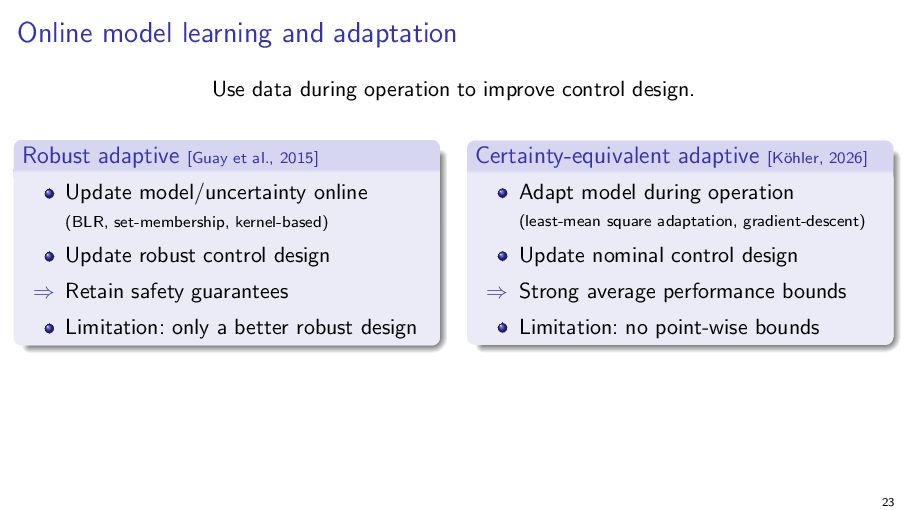
42. Numerical results Drone - certainty-equivalent adaptive tracking MPC [Köhler, 2026] Certainty-equivalent tracking MPC; soft state constraints Drone navigating obstacles Adapt model with simple least-mean square ⇒ Adaptive MPC ensures bounds despite (unknown) time-varying parameters process noise ▶ measurement noise. ▶ ▶ Implementation requires only minimal modification compared to a standard MPC Fast online adaptation crucial for stability. 25
43. Experimental results Repetitive tasks with drone & soft robots [Pabon et al., 2024] Numerical simulations with deformable soft robot Hardware experiments with small racing car 26
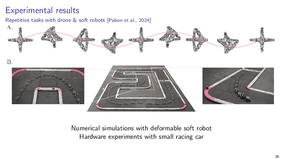
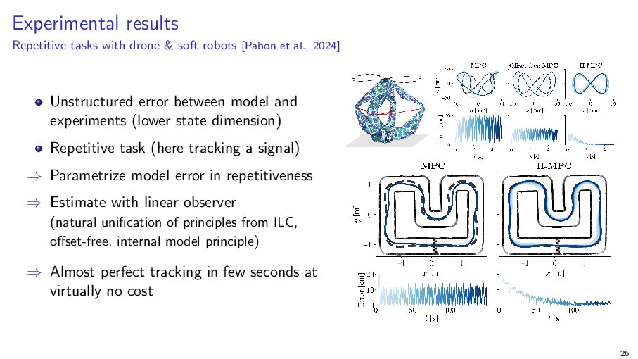
44. Experimental results Repetitive tasks with drone & soft robots [Pabon et al., 2024] Unstructured error between model and experiments (lower state dimension) Repetitive task (here tracking a signal) ⇒ Parametrize model error in repetitiveness ⇒ Estimate with linear observer (natural unification of principles from ILC, offset-free, internal model principle) ⇒ Almost perfect tracking in few seconds at virtually no cost 26
45. Data-driven designs In the following, we will investigate how to: Online model learning/adaptation ▶ use data to improve models online Uncertainty-quantification ▶ obtain realistic bounds on model error from data Data-driven design pipeline ▶ provide a fully automated design pipeline 27
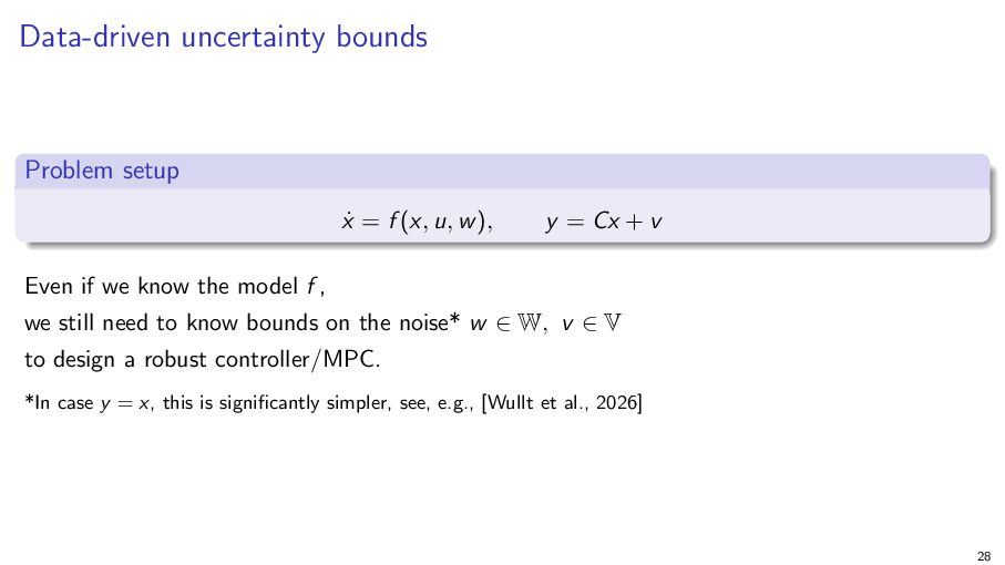
46. Data-driven uncertainty bounds Problem setup ẋ = f (x, u, w ), y = Cx + v Even if we know the model f , we still need to know bounds on the noise* w ∈ W, v ∈ V to design a robust controller/MPC. *In case y = x, this is significantly simpler, see, e.g., [Wullt et al., 2026] 28
47. Data-driven uncertainty bounds [Benders et al., 2025b] 29
48. Data-driven uncertainty bounds [Benders et al., 2025b] Estimating noise bounds We estimate the most likely noise (assuming i.i.d. Gaussian with unknown covariance), ⇒ maximum likelihood estimation (MLE) ⇒ receding-horizon approximation (MHE) ⇒ estimated noise w i , v i ⇒ set W, V 29
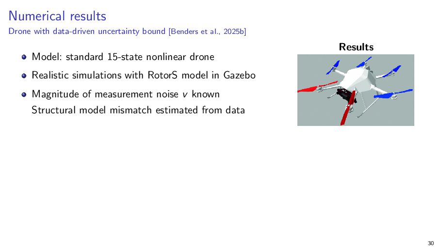
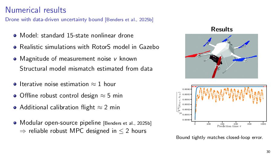
49. Numerical results Drone with data-driven uncertainty bound [Benders et al., 2025b] Model: standard 15-state nonlinear drone Results Realistic simulations with RotorS model in Gazebo Magnitude of measurement noise v known Structural model mismatch estimated from data 30
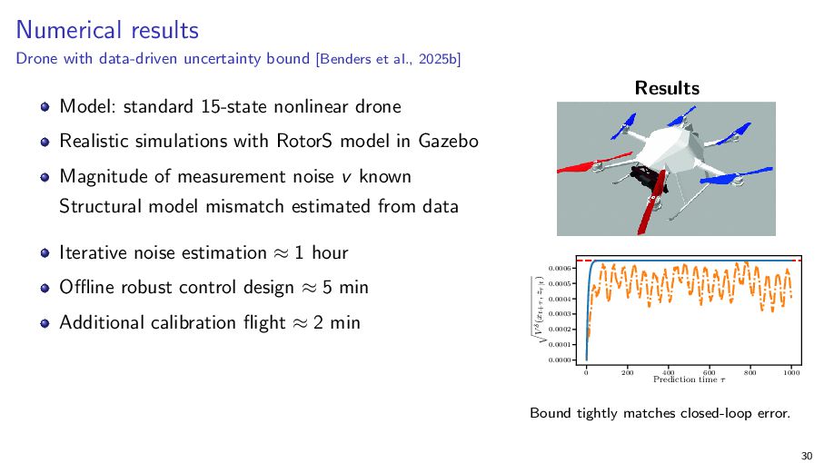
50. Numerical results Drone with data-driven uncertainty bound [Benders et al., 2025b] Results Model: standard 15-state nonlinear drone Realistic simulations with RotorS model in Gazebo Magnitude of measurement noise v known Structural model mismatch estimated from data Iterative noise estimation ≈ 1 hour 0.0005 0.0004 0.0003 0.0002 q Additional calibration flight ≈ 2 min V δ (xt+τ , zτ |t ) 0.0006 Offline robust control design ≈ 5 min 0.0001 0.0000 0 200 400 600 Prediction time τ 800 1000 Bound tightly matches closed-loop error. 30
51. Numerical results Drone with data-driven uncertainty bound [Benders et al., 2025b] Results Model: standard 15-state nonlinear drone Realistic simulations with RotorS model in Gazebo Magnitude of measurement noise v known Structural model mismatch estimated from data Iterative noise estimation ≈ 1 hour 0.0005 0.0004 0.0003 0.0002 q Additional calibration flight ≈ 2 min V δ (xt+τ , zτ |t ) 0.0006 Offline robust control design ≈ 5 min 0.0001 Modular open-source pipeline [Benders et al., 2025b] ⇒ reliable robust MPC designed in ≤ 2 hours 0.0000 0 200 400 600 Prediction time τ 800 1000 Bound tightly matches closed-loop error. 30
52. Data-driven designs In the following, we will investigate how to: Online model learning/adaptation ▶ use data to improve models online Uncertainty-quantification ▶ obtain realistic bounds on model error from data Data-driven design pipeline ▶ provide a fully automated design pipeline 31
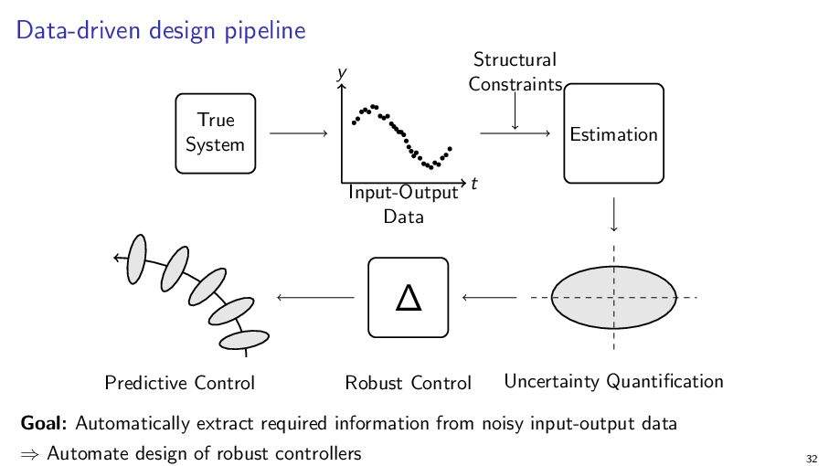
53. Data-driven design pipeline Structural Constraints y True System Estimation Input-Output t Data ∆ Predictive Control Robust Control Uncertainty Quantification Goal: Automatically extract required information from noisy input-output data ⇒ Automate design of robust controllers 32
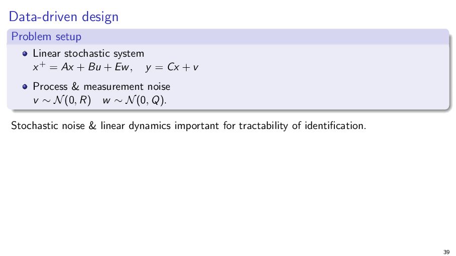
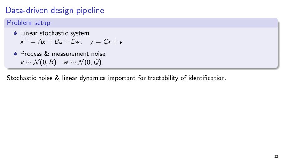
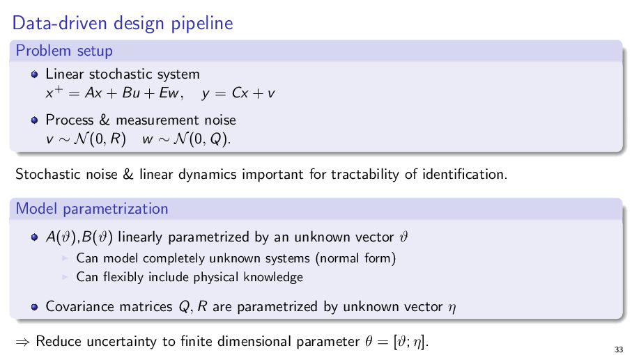
54. Data-driven design pipeline Problem setup Linear stochastic system x + = Ax + Bu + Ew , y = Cx + v Process & measurement noise v ∼ N (0, R) w ∼ N (0, Q). Stochastic noise & linear dynamics important for tractability of identification. 33
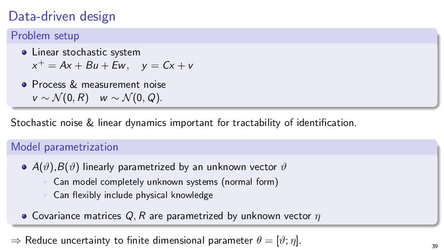
55. Data-driven design pipeline Problem setup Linear stochastic system x + = Ax + Bu + Ew , y = Cx + v Process & measurement noise v ∼ N (0, R) w ∼ N (0, Q). Stochastic noise & linear dynamics important for tractability of identification. Model parametrization A(ϑ),B(ϑ) linearly parametrized by an unknown vector ϑ ▶ ▶ Can model completely unknown systems (normal form) Can flexibly include physical knowledge Covariance matrices Q, R are parametrized by unknown vector η ⇒ Reduce uncertainty to finite dimensional parameter θ = [ϑ; η]. 33
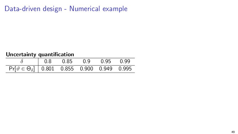
56. Numerical results Data-driven design pipeline [Balim et al., 2024] Numerical results Chain of masses: 10 states, 23 unknown parameters Estimate ϑ̂, Q,R using MLE with GEM: 6 [s] Uncertainty quantification: Pr [ϑ ∈ Θ] = 94.9% ≈ δ = 95% Robust control using full-block S-procedure ∀θ ∈ Θ: 6 [s] MPC: ensures probabilistic constraints with stochastic noise and parametric uncertainty Automated design of controller from data in few seconds Provide performance and safety guarantees despite uncertainty 34
57. Data-driven design pipeline Limitation What about an automated data-driven design for nonlinear systems? 35
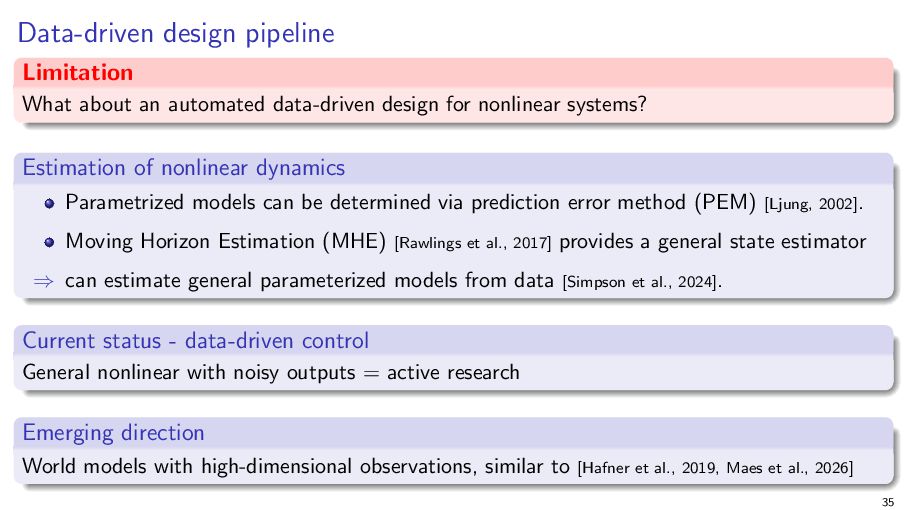
58. Data-driven design pipeline Limitation What about an automated data-driven design for nonlinear systems? Estimation of nonlinear dynamics Parametrized models can be determined via prediction error method (PEM) [Ljung, 2002]. Moving Horizon Estimation (MHE) [Rawlings et al., 2017] provides a general state estimator ⇒ can estimate general parameterized models from data [Simpson et al., 2024]. Current status - data-driven control General nonlinear with noisy outputs = active research Emerging direction World models with high-dimensional observations, similar to [Hafner et al., 2019, Maes et al., 2026] 35
59. Conclusion MPC: optimization-based control ⇒ Performance/stability & constraint satisfaction 36
60. Conclusion MPC: optimization-based control ⇒ Performance/stability & constraint satisfaction Robust designs - via contraction metrics Account for model uncertainty ⇒ Robust guarantees: constraint satisfaction, performance, stability 36
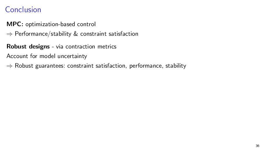
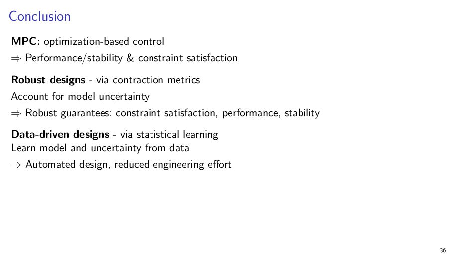
61. Conclusion MPC: optimization-based control ⇒ Performance/stability & constraint satisfaction Robust designs - via contraction metrics Account for model uncertainty ⇒ Robust guarantees: constraint satisfaction, performance, stability Data-driven designs - via statistical learning Learn model and uncertainty from data ⇒ Automated design, reduced engineering effort 36
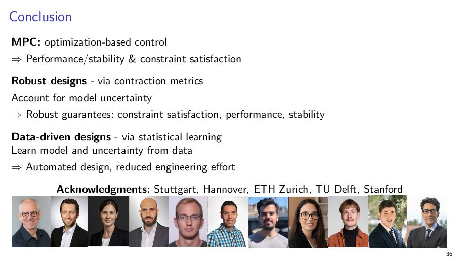
62. Conclusion MPC: optimization-based control ⇒ Performance/stability & constraint satisfaction Robust designs - via contraction metrics Account for model uncertainty ⇒ Robust guarantees: constraint satisfaction, performance, stability Data-driven designs - via statistical learning Learn model and uncertainty from data ⇒ Automated design, reduced engineering effort Acknowledgments: Stuttgart, Hannover, ETH Zurich, TU Delft, Stanford 36
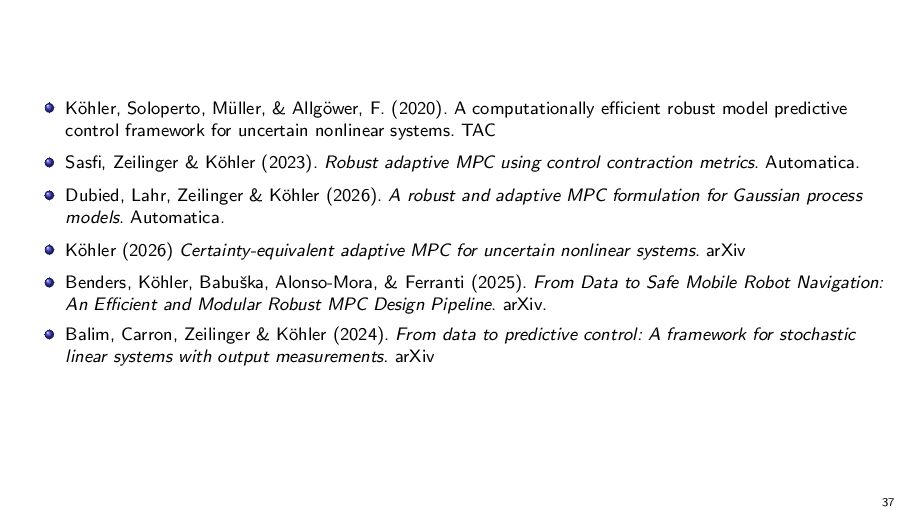
63. Köhler, Soloperto, Müller, & Allgöwer, F. (2020). A computationally efficient robust model predictive control framework for uncertain nonlinear systems. TAC Sasfi, Zeilinger & Köhler (2023). Robust adaptive MPC using control contraction metrics. Automatica. Dubied, Lahr, Zeilinger & Köhler (2026). A robust and adaptive MPC formulation for Gaussian process models. Automatica. Köhler (2026) Certainty-equivalent adaptive MPC for uncertain nonlinear systems. arXiv Benders, Köhler, Babuška, Alonso-Mora, & Ferranti (2025). From Data to Safe Mobile Robot Navigation: An Efficient and Modular Robust MPC Design Pipeline. arXiv. Balim, Carron, Zeilinger & Köhler (2024). From data to predictive control: A framework for stochastic linear systems with output measurements. arXiv 37
64. Alora, J. I., Pabon, L. A., Köhler, J., Cenedese, M., Schmerling, E., Zeilinger, M. N., Haller, G., and Pavone, M. (2023). Robust nonlinear reduced-order model predictive control. In Proc. 62nd IEEE Conference on Decision and Control (CDC), pages 4798–4805. IEEE. Angeli, D., Amrit, R., and Rawlings, J. B. (2011). On average performance and stability of economic model predictive control. IEEE transactions on automatic control, 57(7):1615–1626. Ao, Y., Köhler, J., Prajapat, M., As, Y., Zeilinger, M., Fürnstahl, P., and Krause, A. (2025). Stochastic model predictive control for sub-gaussian noise. arXiv preprint arXiv:2503.08795. Arcari, E., Iannelli, A., Carron, A., and Zeilinger, M. N. (2023). Stochastic mpc with robustness to bounded parameteric uncertainty. IEEE Transactions on Automatic Control, 68(12):7601–7615. Arnström, D. (2023). Real-time Certified MPC Reliable Active-Set QP Solvers. Linkopings Universitet (Sweden). Balim, H., Carron, A., Zeilinger, M. N., and Köhler, J. (2024). From data to predictive control: A framework for stochastic linear systems with output measurements. arXiv preprint arXiv:2407.17277. Benders, D., Ferranti, L., and Köhler, J. (2025a). A step-by-step guide on nonlinear model predictive control for safe mobile robot navigation. 37
65. arXiv preprint arXiv:2507.17856. Benders, D., Köhler, J., Babuška, R., Alonso-Mora, J., and Ferranti, L. (2025b). From data to safe mobile robot navigation: An efficient and modular robust MPC design pipeline. arXiv preprint arXiv:2508.07045. Benders, D., Köhler, J., Niesten, T., Babuška, R., Alonso-Mora, J., and Ferranti, L. (2025c). Embedded hierarchical MPC for autonomous navigation. IEEE Transactions on Robotics. Brunke, L., Zhou, S., and Schoellig, A. P. (2022). Robust predictive output-feedback safety filter for uncertain nonlinear control systems. In 2022 IEEE 61st Conference on Decision and Control (CDC), pages 3051–3058. IEEE. Cramér, H. (1999). Mathematical methods of statistics, volume 43. Princeton university press. Degner, M., Soloperto, R., Zeilinger, M. N., Lygeros, J., and Köhler, J. (2026). Adaptive economic model predictive control: Performance guarantees for nonlinear systems. IEEE Trans. Autom. Control. Dubied, M., Lahr, A., Zeilinger, M. N., and Köhler, J. (2026). A robust and adaptive mpc formulation for gaussian process models. Automatica, 194:113276. Eberhard, P. B., Köhler, J., Hüsser, O., Zeilinger, M. N., and Carron, A. (2025). Time-varying coverage control: A distributed tracker-planner mpc framework. 37
66. arXiv preprint arXiv:2507.01567. Forni, F. and Sepulchre, R. (2013). A differential lyapunov framework for contraction analysis. IEEE transactions on automatic control, 59(3):614–628. Fromion, V. and Scorletti, G. (2003). A theoretical framework for gain scheduling. International Journal of Robust and Nonlinear Control: IFAC-Affiliated Journal, 13(10):951–982. Gibson, S. and Ninness, B. (2005). Robust maximum-likelihood estimation of multivariable dynamic systems. Automatica, 41(10):1667–1682. Grüne, L. and Pannek, J. (2017). Nonlinear Model Predictive Control. Springer. Guay, M., Adetola, V., and DeHaan, D. (2015). Robust and Adaptive Model Predictive Control of Nonlinear Systems. Institution of Engineering and Technology. Hafner, D., Lillicrap, T., Ba, J., and Norouzi, M. (2019). Dream to control: Learning behaviors by latent imagination. arXiv preprint arXiv:1912.01603. Hertneck, M., Köhler, J., Trimpe, S., and Allgöwer, F. (2018). Learning an approximate model predictive controller with guarantees. 37
67. IEEE Control Systems Letters, 2(3):543–548. Hose, H., Köhler, J., Zeilinger, M. N., and Trimpe, S. (2025). Approximate nonlinear model predictive control with safety-augmented neural networks. IEEE Transactions on Control Systems Technology. Koelewijn, P., Tóth, R., and Nijmeijer, H. (2019). Linear parameter-varying control of nonlinear systems based on incremental stability. IFAC-PapersOnLine, 52(28):38–43. Köhler, J. (2021). Analysis and design of MPC frameworks for dynamic operation of nonlinear constrained systems. PhD thesis, Universität Stuttgart. doi:10.18419/opus-11742. Köhler, J. (2026). Certainty-equivalent adaptive MPC for uncertain nonlinear systems. arXiv preprint arXiv:2603.17843. Köhler, J., Allgöwer, F., and Müller, M. A. (2019a). A simple framework for nonlinear robust output-feedback MPC. In Proc. 18th European Control Conference (ECC), pages 793–798. IEEE. Köhler, J., Kötting, P., Soloperto, R., Allgöwer, F., and Müller, M. A. (2021a). A robust adaptive model predictive control framework for nonlinear uncertain systems. International Journal of Robust and Nonlinear Control, 31(18):8725–8749. Köhler, J., Müller, M. A., and Allgöwer, F. (2019b). 37
68. A nonlinear model predictive control framework using reference generic terminal ingredients. IEEE Transactions on Automatic Control, 65(8):3576–3583. Köhler, J., Müller, M. A., and Allgöwer, F. (2020). Periodic optimal control of nonlinear constrained systems using economic model predictive control. Journal of Process Control, 92:185–201. Köhler, J., Müller, M. A., and Allgöwer, F. (2021b). Robust output feedback model predictive control using online estimation bounds. arXiv preprint arXiv:2105.03427. Köhler, J., Müller, M. A., and Allgöwer, F. (2024). Analysis and design of model predictive control frameworks for dynamic operation—an overview. Annual Reviews in Control, 57:100929. Köhler, J., Scholz, C., and Zeilinger, M. (2026). Robust reduced-order model predictive control using peak-to-peak analysis of filtered signals. European Journal of Control, page 101569. Köhler, J., Soloperto, R., Müller, M. A., and Allgöwer, F. (2021). A computationally efficient robust model predictive control framework for uncertain nonlinear systems. IEEE Trans. Automat. Control, 66(2):794–801. Köhler, J. and Zeilinger, M. N. (2025). Predictive control for nonlinear stochastic systems: Closed-loop guarantees with unbounded noise. IEEE Transactions on Automatic Control. Köhler, J., Zhang, D., Soloperto, R., Carron, A., and Zeilinger, M. (2025). 37
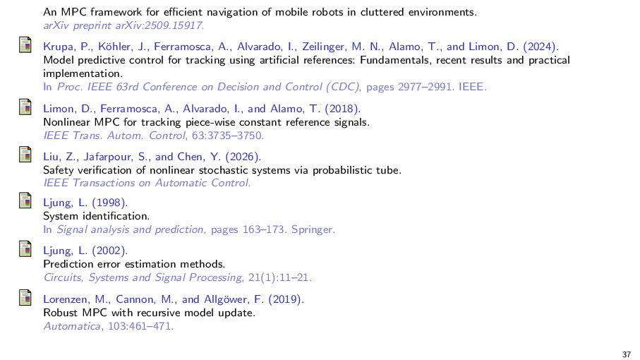
69. An MPC framework for efficient navigation of mobile robots in cluttered environments. arXiv preprint arXiv:2509.15917. Krupa, P., Köhler, J., Ferramosca, A., Alvarado, I., Zeilinger, M. N., Alamo, T., and Limon, D. (2024). Model predictive control for tracking using artificial references: Fundamentals, recent results and practical implementation. In Proc. IEEE 63rd Conference on Decision and Control (CDC), pages 2977–2991. IEEE. Limon, D., Ferramosca, A., Alvarado, I., and Alamo, T. (2018). Nonlinear MPC for tracking piece-wise constant reference signals. IEEE Trans. Autom. Control, 63:3735–3750. Liu, Z., Jafarpour, S., and Chen, Y. (2026). Safety verification of nonlinear stochastic systems via probabilistic tube. IEEE Transactions on Automatic Control. Ljung, L. (1998). System identification. In Signal analysis and prediction, pages 163–173. Springer. Ljung, L. (2002). Prediction error estimation methods. Circuits, Systems and Signal Processing, 21(1):11–21. Lorenzen, M., Cannon, M., and Allgöwer, F. (2019). Robust MPC with recursive model update. Automatica, 103:461–471. 37
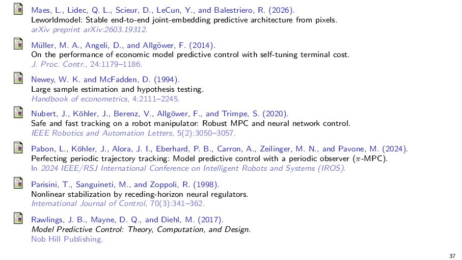
70. Maes, L., Lidec, Q. L., Scieur, D., LeCun, Y., and Balestriero, R. (2026). Leworldmodel: Stable end-to-end joint-embedding predictive architecture from pixels. arXiv preprint arXiv:2603.19312. Müller, M. A., Angeli, D., and Allgöwer, F. (2014). On the performance of economic model predictive control with self-tuning terminal cost. J. Proc. Contr., 24:1179–1186. Newey, W. K. and McFadden, D. (1994). Large sample estimation and hypothesis testing. Handbook of econometrics, 4:2111–2245. Nubert, J., Köhler, J., Berenz, V., Allgöwer, F., and Trimpe, S. (2020). Safe and fast tracking on a robot manipulator: Robust MPC and neural network control. IEEE Robotics and Automation Letters, 5(2):3050–3057. Pabon, L., Köhler, J., Alora, J. I., Eberhard, P. B., Carron, A., Zeilinger, M. N., and Pavone, M. (2024). Perfecting periodic trajectory tracking: Model predictive control with a periodic observer (π-MPC). In 2024 IEEE/RSJ International Conference on Intelligent Robots and Systems (IROS). Parisini, T., Sanguineti, M., and Zoppoli, R. (1998). Nonlinear stabilization by receding-horizon neural regulators. International Journal of Control, 70(3):341–362. Rawlings, J. B., Mayne, D. Q., and Diehl, M. (2017). Model Predictive Control: Theory, Computation, and Design. Nob Hill Publishing. 37
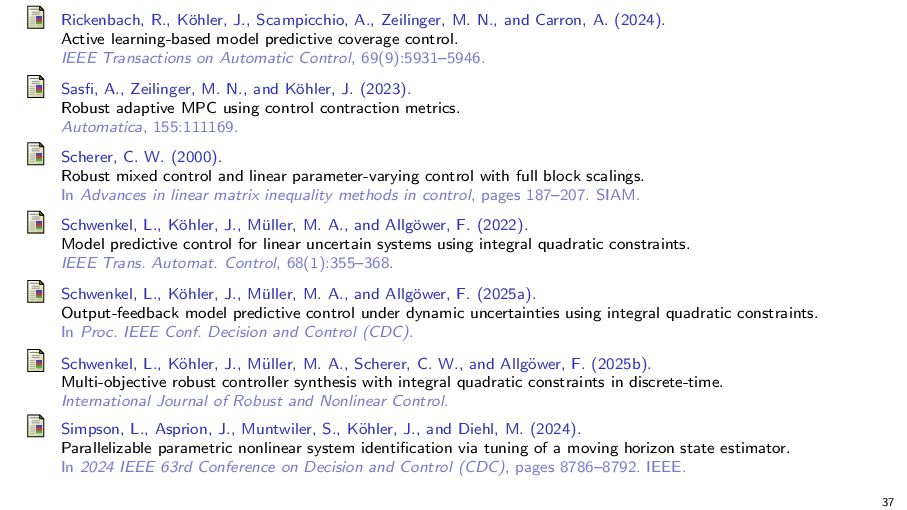
71. Rickenbach, R., Köhler, J., Scampicchio, A., Zeilinger, M. N., and Carron, A. (2024). Active learning-based model predictive coverage control. IEEE Transactions on Automatic Control, 69(9):5931–5946. Sasfi, A., Zeilinger, M. N., and Köhler, J. (2023). Robust adaptive MPC using control contraction metrics. Automatica, 155:111169. Scherer, C. W. (2000). Robust mixed control and linear parameter-varying control with full block scalings. In Advances in linear matrix inequality methods in control, pages 187–207. SIAM. Schwenkel, L., Köhler, J., Müller, M. A., and Allgöwer, F. (2022). Model predictive control for linear uncertain systems using integral quadratic constraints. IEEE Trans. Automat. Control, 68(1):355–368. Schwenkel, L., Köhler, J., Müller, M. A., and Allgöwer, F. (2025a). Output-feedback model predictive control under dynamic uncertainties using integral quadratic constraints. In Proc. IEEE Conf. Decision and Control (CDC). Schwenkel, L., Köhler, J., Müller, M. A., Scherer, C. W., and Allgöwer, F. (2025b). Multi-objective robust controller synthesis with integral quadratic constraints in discrete-time. International Journal of Robust and Nonlinear Control. Simpson, L., Asprion, J., Muntwiler, S., Köhler, J., and Diehl, M. (2024). Parallelizable parametric nonlinear system identification via tuning of a moving horizon state estimator. In 2024 IEEE 63rd Conference on Decision and Control (CDC), pages 8786–8792. IEEE. 37
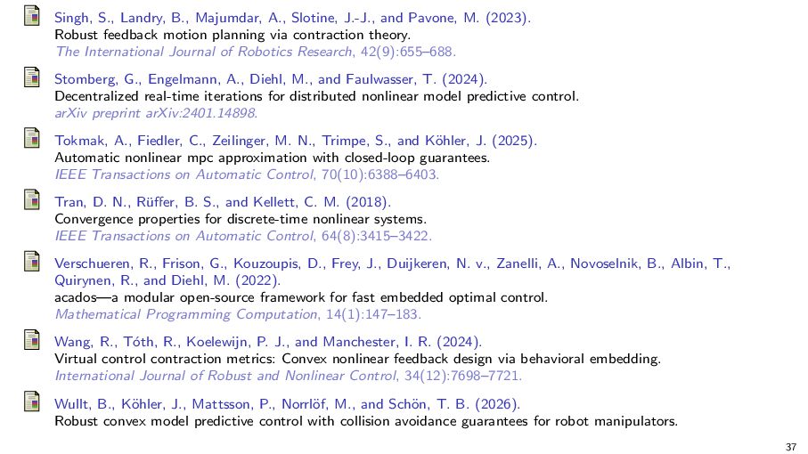
72. Singh, S., Landry, B., Majumdar, A., Slotine, J.-J., and Pavone, M. (2023). Robust feedback motion planning via contraction theory. The International Journal of Robotics Research, 42(9):655–688. Stomberg, G., Engelmann, A., Diehl, M., and Faulwasser, T. (2024). Decentralized real-time iterations for distributed nonlinear model predictive control. arXiv preprint arXiv:2401.14898. Tokmak, A., Fiedler, C., Zeilinger, M. N., Trimpe, S., and Köhler, J. (2025). Automatic nonlinear mpc approximation with closed-loop guarantees. IEEE Transactions on Automatic Control, 70(10):6388–6403. Tran, D. N., Rüffer, B. S., and Kellett, C. M. (2018). Convergence properties for discrete-time nonlinear systems. IEEE Transactions on Automatic Control, 64(8):3415–3422. Verschueren, R., Frison, G., Kouzoupis, D., Frey, J., Duijkeren, N. v., Zanelli, A., Novoselnik, B., Albin, T., Quirynen, R., and Diehl, M. (2022). acados—a modular open-source framework for fast embedded optimal control. Mathematical Programming Computation, 14(1):147–183. Wang, R., Tóth, R., Koelewijn, P. J., and Manchester, I. R. (2024). Virtual control contraction metrics: Convex nonlinear feedback design via behavioral embedding. International Journal of Robust and Nonlinear Control, 34(12):7698–7721. Wullt, B., Köhler, J., Mattsson, P., Norrlöf, M., and Schön, T. B. (2026). Robust convex model predictive control with collision avoidance guarantees for robot manipulators. 37
73. IEEE Transactions on Control Systems Technology. Zhao, P., Lakshmanan, A., Ackerman, K., Gahlawat, A., Pavone, M., and Hovakimyan, N. (2022). Tube-certified trajectory tracking for nonlinear systems with robust control contraction metrics. IEEE Robotics and Automation Letters, 7(2):5528–5535. extended version on arXiv:2109.04453. 38
74. Appendix -Data-driven MPC 38
75. Data-driven design Problem setup Linear stochastic system x + = Ax + Bu + Ew , y = Cx + v Process & measurement noise v ∼ N (0, R) w ∼ N (0, Q). Stochastic noise & linear dynamics important for tractability of identification. 39
76. Data-driven design Problem setup Linear stochastic system x + = Ax + Bu + Ew , y = Cx + v Process & measurement noise v ∼ N (0, R) w ∼ N (0, Q). Stochastic noise & linear dynamics important for tractability of identification. Model parametrization A(ϑ),B(ϑ) linearly parametrized by an unknown vector ϑ ▶ ▶ Can model completely unknown systems (normal form) Can flexibly include physical knowledge Covariance matrices Q, R are parametrized by unknown vector η ⇒ Reduce uncertainty to finite dimensional parameter θ = [ϑ; η]. 39
77. Data-driven design - Identification Maximum likelihood estimation (MLE) [Ljung, 1998, Cramér, 1999]: ▶ ▶ θ̂ = arg maxθ L(θ|Data) MLE has no closed-form solution, since the states x are not known 40
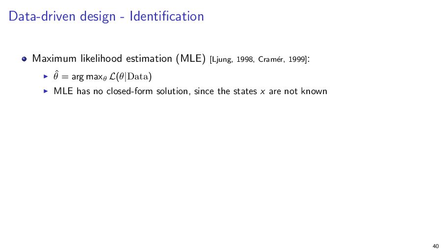
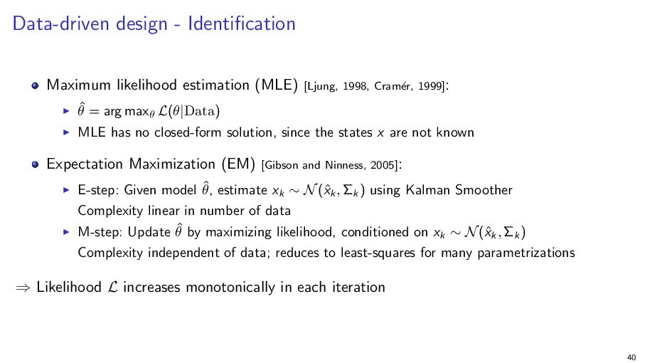
78. Data-driven design - Identification Maximum likelihood estimation (MLE) [Ljung, 1998, Cramér, 1999]: ▶ ▶ θ̂ = arg maxθ L(θ|Data) MLE has no closed-form solution, since the states x are not known Expectation Maximization (EM) [Gibson and Ninness, 2005]: E-step: Given model θ̂, estimate xk ∼ N (x̂k , Σk ) using Kalman Smoother Complexity linear in number of data ▶ M-step: Update θ̂ by maximizing likelihood, conditioned on x ∼ N (x̂ , Σ ) k k k Complexity independent of data; reduces to least-squares for many parametrizations ▶ ⇒ Likelihood L increases monotonically in each iteration 40
79. Data-driven design - Uncertainty quantification MLE is a consistent estimator Error asymptotically* Gaussian [Ljung, 1998]: ϑ − ϑ̂ ∼ N (0, Σϑ ); Σϑ = − ∂2 log(L(ϑ))|ϑ̂ ∂ϑ2 ⇒ Confidence set: Pr [ϑ ∈ Θ] ≥ δ ⇒ Data-driven uncertainty characterization: Noise covariances Q(η̂), R(η̂) Parametric uncertainty ϑ ∈ Θ *Assuming identifiability and persistence of excitation, we have Σϑ ≻ 0. Distribution approaches Gaussian as the number of data points increases. Evaluation of Hessian at estimate ϑ̂ converges to evaluation at unknown true ϑ, cf. [Newey and McFadden, 1994]. 41
80. Data-driven design - Robust control Structured uncertainty [Balim et al., 2024] A(ϑ) = Â + E · ∆ · J∆ with uncertainty ∆ = I ⊗ (ϑ − ϑ̂)⊤ ∈ Rnw ×nw nϑ . ∆∈∆⇔ϑ∈Θ )  ⊤  ⊤ ⊤ ∆ ∆ P∆ ⪰ 0 ∀P∆ ∈ P∆ Uncertainty set: ∆ = ∆| I I    −Λ ⊗ Σ−1 0 ϑ,δ Multipliers: P∆ = | Λ⪰0 0 Λ ( ⇒ Can use robust control synthesis with full-block S-procedure [Scherer, 2000] ⇒ Output-feedback controller guarantees stability and H2 -norm for uncertain system 42
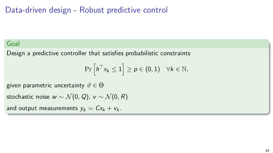
81. Data-driven design - Robust predictive control Goal Design a predictive controller that satisfies probabilistic constraints h i Pr h⊤ xk ≤ 1 ≥ p ∈ (0, 1) ∀k ∈ N, given parametric uncertainty ϑ ∈ Θ stochastic noise w ∼ N (0, Q), v ∼ N (0, R) and output measurements yk = Cxk + vk . 43
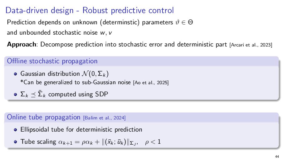
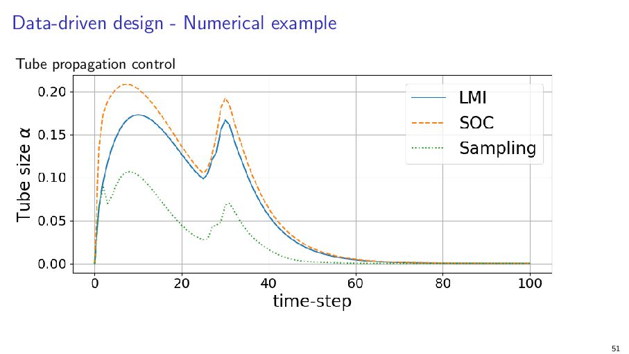
82. Data-driven design - Robust predictive control Prediction depends on unknown (determinstic) parameters ϑ ∈ Θ and unbounded stochastic noise w , v Approach: Decompose prediction into stochastic error and deterministic part [Arcari et al., 2023] Offline stochastic propagation Gaussian distribution N (0, Σk ) *Can be generalized to sub-Gaussian noise [Ao et al., 2025] Σk ⪯ Σ̄k computed using SDP Online tube propagation [Balim et al., 2024] Ellipsoidal tube for deterministic prediction Tube scaling αk+1 = ραk + ∥(x̄k ; ūk )∥ΣJ , ρ<1 44
83. Data-driven design - Robust predictive control MPC formulation min Cost on nominal prediction s.t. Tube dynamics Tightened constraints Terminal constraint Initial state constraints 45
84. Data-driven design - Robust predictive control Theorem [Balim et al., 2024] Given uncertainty description; MPC formulation min Cost on nominal prediction s.t. Tube dynamics Feasibility of MPC at t=0. Then, the closed-loop systems satisfies Recursive feasibility Tightened constraints Chance constraints Terminal constraint Performance bound "N−1 # X 1 2 2 lim E ∥xt ∥Qc + ∥ut ∥Rc ≤ γ 2 . N→∞ N Initial state constraints t=0 45
85. Data-driven design - Robust predictive control min ν , ·|t ξ̄·|t , α·|t T −1 X (∥ξ¯i|t ∥2Qξ,c + ∥νi|t ∥2Rc ) + ∥ξ¯T |t ∥Sξ,c (1a) i=0 s.t. ξ¯i+1|t = Âξ¯i|t + B̂ν νi|t , tube dynamics: 1/2 αi+1|t ≥ ραi|t + Σ̄J,ϑ,δ (1b)  x̄i|t ūi|t  (1c) , tightened constraints:     0 I 0 ¯ ⊤ hj ξ + ≤ 1 − cj,t+i − αi|t fj , νi|t 0 K i|t terminal constraint: (ξ¯T |t , αT |t ) ∈ Ω, (1d) ⋆ ⋆ initial state: α0|t = α1|t−1 , ξ¯0|t = ξ¯1|t−1 . (1f) (1e) 46
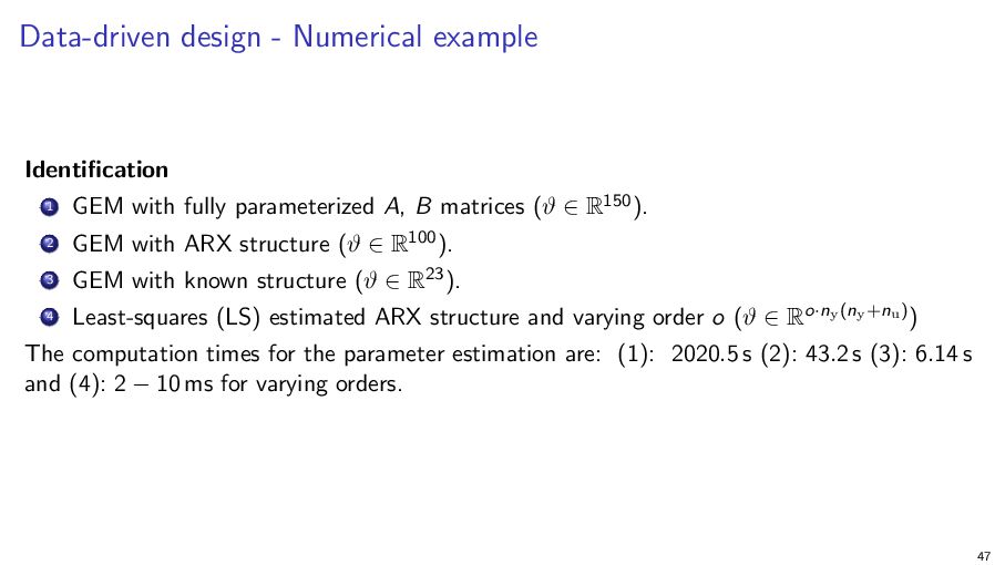
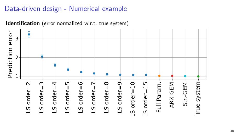
86. Data-driven design - Numerical example Identification 1 GEM with fully parameterized A, B matrices (ϑ ∈ R150 ). 2 GEM with ARX structure (ϑ ∈ R100 ). 3 GEM with known structure (ϑ ∈ R23 ). 4 Least-squares (LS) estimated ARX structure and varying order o (ϑ ∈ Ro·ny (ny +nu ) ) The computation times for the parameter estimation are: (1): 2020.5 s (2): 43.2 s (3): 6.14 s and (4): 2 − 10 ms for varying orders. 47
87. Data-driven design - Numerical example Identification (error normalized w.r.t. true system) 48
88. Data-driven design - Numerical example Uncertainty quantification δ 0.8 0.85 Pr[ϑ ∈ Θδ ] 0.801 0.855 0.9 0.900 0.95 0.949 0.99 0.995 49
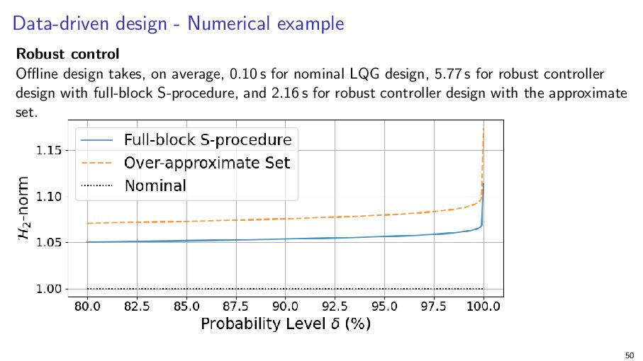
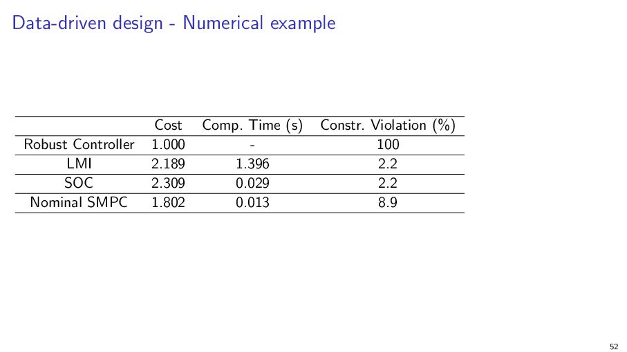
89. Data-driven design - Numerical example Robust control Offline design takes, on average, 0.10 s for nominal LQG design, 5.77 s for robust controller design with full-block S-procedure, and 2.16 s for robust controller design with the approximate set. 50
90. Data-driven design - Numerical example Tube propagation control 51
91. Data-driven design - Numerical example Robust Controller LMI SOC Nominal SMPC Cost 1.000 2.189 2.309 1.802 Comp. Time (s) 1.396 0.029 0.013 Constr. Violation (%) 100 2.2 2.2 8.9 52