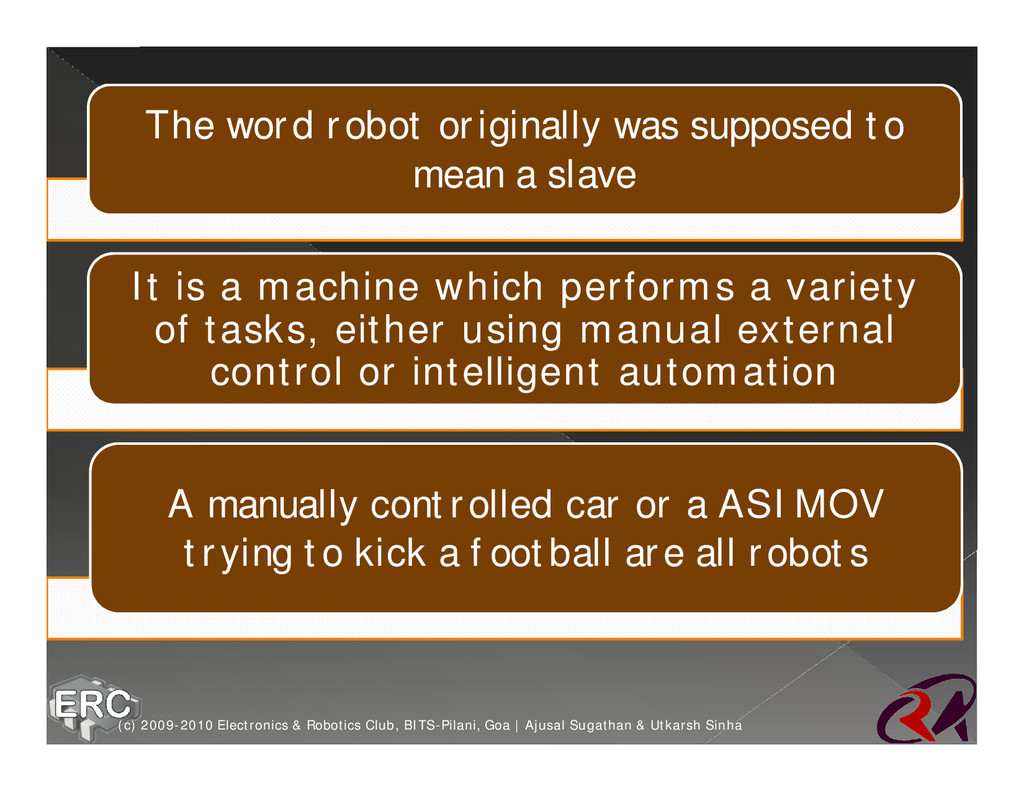
It is a machine which performs a variety of tasks, either using manual external control or intelligent automation A manually controlled car or a ASIMOV trying to kick a football are all robots (c) 2009-2010 Electronics & Robotics Club, BITS-Pilani, Goa | Ajusal Sugathan & Utkarsh Sinha
the vistas of › Mechanical design › Electronic control › Artificial Intelligence ž It finds it’s uses in all aspects of our life › automated vacuum cleaner › Exploring the ‘Red’ planet › Setting up a human colony there :D (c) 2009-2010 Electronics & Robotics Club, BITS-Pilani, Goa | Ajusal Sugathan & Utkarsh Sinha
it move. Ob. Ø This system gives our machine the ability to move forward, backward and take turns Ø It may also provide for climbing up and down Ø Or even flying or floating J (c) 2009-2010 Electronics & Robotics Club, BITS-Pilani, Goa | Ajusal Sugathan & Utkarsh Sinha
of freedom Ø More degrees of freedom means more the number of actuators you will have to use Ø Although one actuator can be used to control more than one degree of freedom (c) 2009-2010 Electronics & Robotics Club, BITS-Pilani, Goa | Ajusal Sugathan & Utkarsh Sinha
at the undergrad level Ø This involves conversion of electrical energy into mechanical energy (mostly using motors) Ø The issue is to control these motors to give the required speed and torque (c) 2009-2010 Electronics & Robotics Club, BITS-Pilani, Goa | Ajusal Sugathan & Utkarsh Sinha
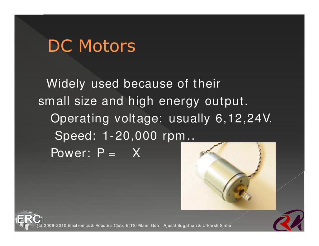
delivered to the motor: › P = ζ X ω Ø Note that the torque and angular velocity are inversely proportionally to each other Ø So to increase the speed we have to reduce the torque (c) 2009-2010 Electronics & Robotics Club, BITS-Pilani, Goa | Ajusal Sugathan & Utkarsh Sinha
rotation which is generally not needed Ø At high speeds, they lack torque Ø For reduction in speed and increase in “pulling capacity” we use pulley or gear systems (c) 2009-2010 Electronics & Robotics Club, BITS-Pilani, Goa | Ajusal Sugathan & Utkarsh Sinha
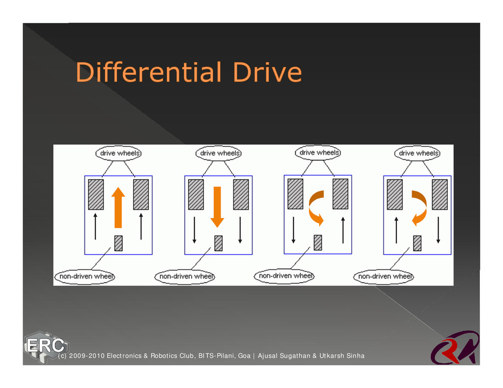
It has a free moving wheel in the front accompanied with a left and right wheel. The two wheels are separately powered Ø When the wheels move in the same direction the machine moves in that direction. Ø Turning is achieved by making the wheels oppose each other’s motion, thus generating a couple (c) 2009-2010 Electronics & Robotics Club, BITS-Pilani, Goa | Ajusal Sugathan & Utkarsh Sinha
the drive wheels at the same rate in the opposite direction Ø Arbitrary motion paths can be implemented by dynamically modifying the angular velocity and/or direction of the drive wheels Ø Total of two motors are required, both of them are responsible for translation and rotational motion (c) 2009-2010 Electronics & Robotics Club, BITS-Pilani, Goa | Ajusal Sugathan & Utkarsh Sinha
preferred system by beginners Ø Independent drives makes it difficult for straight line motion. The differences in motors and frictional profile of the two wheels cause them to move with slight turning effect Ø The above drawback must be countered with appropriate feedback system. Suitable for human controlled remote robots (c) 2009-2010 Electronics & Robotics Club, BITS-Pilani, Goa | Ajusal Sugathan & Utkarsh Sinha
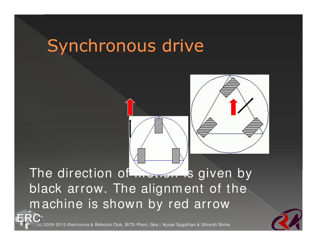
& turns Ø It is made up of a system of 2 motors. One which drive the wheels and the other turns the wheels in a synchronous fashion Ø The two can be directly mechanically coupled as they always move in the same direction with same speed (c) 2009-2010 Electronics & Robotics Club, BITS-Pilani, Goa | Ajusal Sugathan & Utkarsh Sinha
turning guarantees straight line motion without the need for dynamic feedback control Ø This system is somewhat complex in designing but further use is much simpler (c) 2009-2010 Electronics & Robotics Club, BITS-Pilani, Goa | Ajusal Sugathan & Utkarsh Sinha
robots to move. Ø Most actuators are powered by pneumatics (air pressure), hydraulics (fluid pressure), or motors (electric current). Ø They are devices which transform an input signal (mainly an electrical signal)) into motion (c) 2009-2010 Electronics & Robotics Club, BITS-Pilani, Goa | Ajusal Sugathan & Utkarsh Sinha
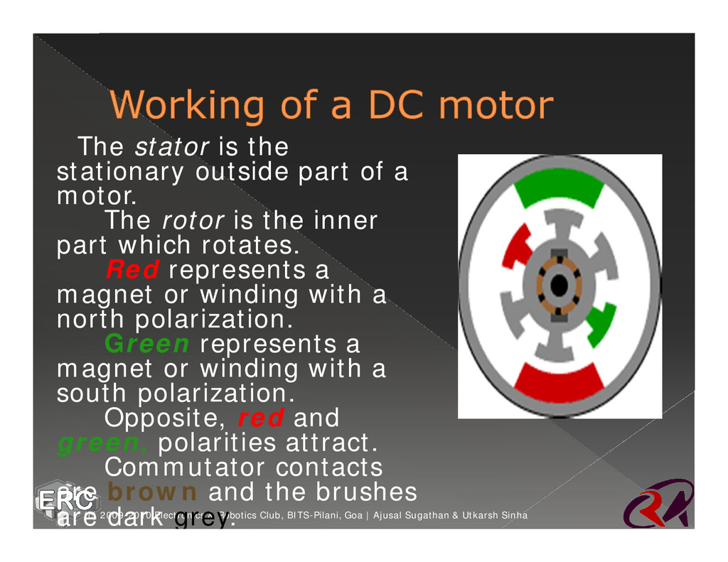
Sugathan & Utkarsh Sinha ØThe stator is the stationary outside part of a motor. Ø The rotor is the inner part which rotates. Ø Red represents a magnet or winding with a north polarization. Ø Green represents a magnet or winding with a south polarization. Ø Opposite, red and green, polarities attract. Ø Commutator contacts are brown and the brushes are dark grey.
Sugathan & Utkarsh Sinha Ø Stator is composed of two or more permanent magnet pole pieces. Ø Rotor composed of windings which are connected to a mechanical commutator. Ø The opposite polarities of the energized winding and the stator magnet attract and the rotor will rotate until it is aligned with the stator. Ø Just as the rotor reaches alignment, the brushes move across the commutator contacts and energize the next winding. Ø A yellow spark shows when the brushes switch to the next winding.
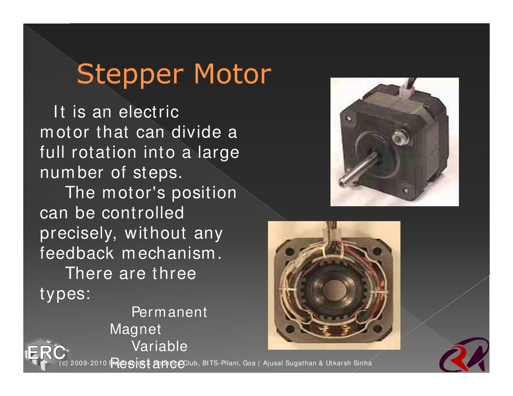
Sugathan & Utkarsh Sinha ØIt is an electric motor that can divide a full rotation into a large number of steps. Ø The motor's position can be controlled precisely, without any feedback mechanism. Ø There are three types: Ø Permanent Magnet Ø Variable Resistance Ø Hybrid type
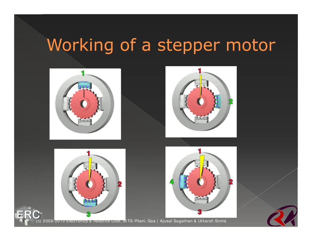
Sugathan & Utkarsh Sinha Ø Stepper motors work in a similar way to dc motors, but where dc motors have 1 electromagnetic coil to produce movement, stepper motors contain many. Ø Stepper motors are controlled by turning each coil on and off in a sequence. Ø Every time a new coil is energized, the motor rotates a few degrees, called the step angle.
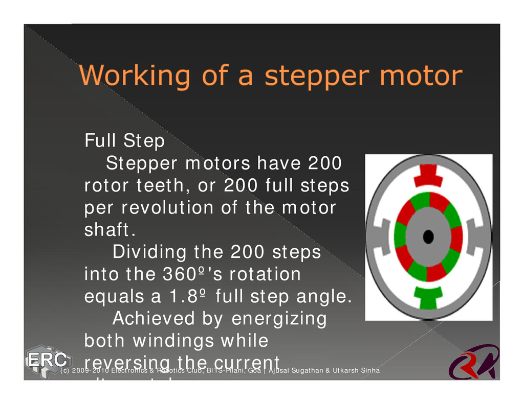
Sugathan & Utkarsh Sinha Full Step Ø Stepper motors have 200 rotor teeth, or 200 full steps per revolution of the motor shaft. Ø Dividing the 200 steps into the 360º's rotation equals a 1.8º full step angle. Ø Achieved by energizing both windings while reversing the current alternately.
Sugathan & Utkarsh Sinha ØServos operate on the principle of negative feedback, where the control input is compared to the actual position of the mechanical system as measured. ØAny difference between the actual and wanted values (an "error signal") is amplified and used to drive the system in the direction necessary to reduce or eliminate the error ØTheir precision movement makes them ideal for powering legs, controlling rack and pinion steering, to move a sensor around etc.
Ø Mobile robots are most suitably powered by batteries Ø The weight and energy capacity of the batteries may become the determinative factor of its performance (c) 2009-2010 Electronics & Robotics Club, BITS-Pilani, Goa | Ajusal Sugathan & Utkarsh Sinha
or voltage eliminators (convert the normal 220V supply to the required DC voltage 12V , 24V etc.) (c) 2009-2010 Electronics & Robotics Club, BITS-Pilani, Goa | Ajusal Sugathan & Utkarsh Sinha
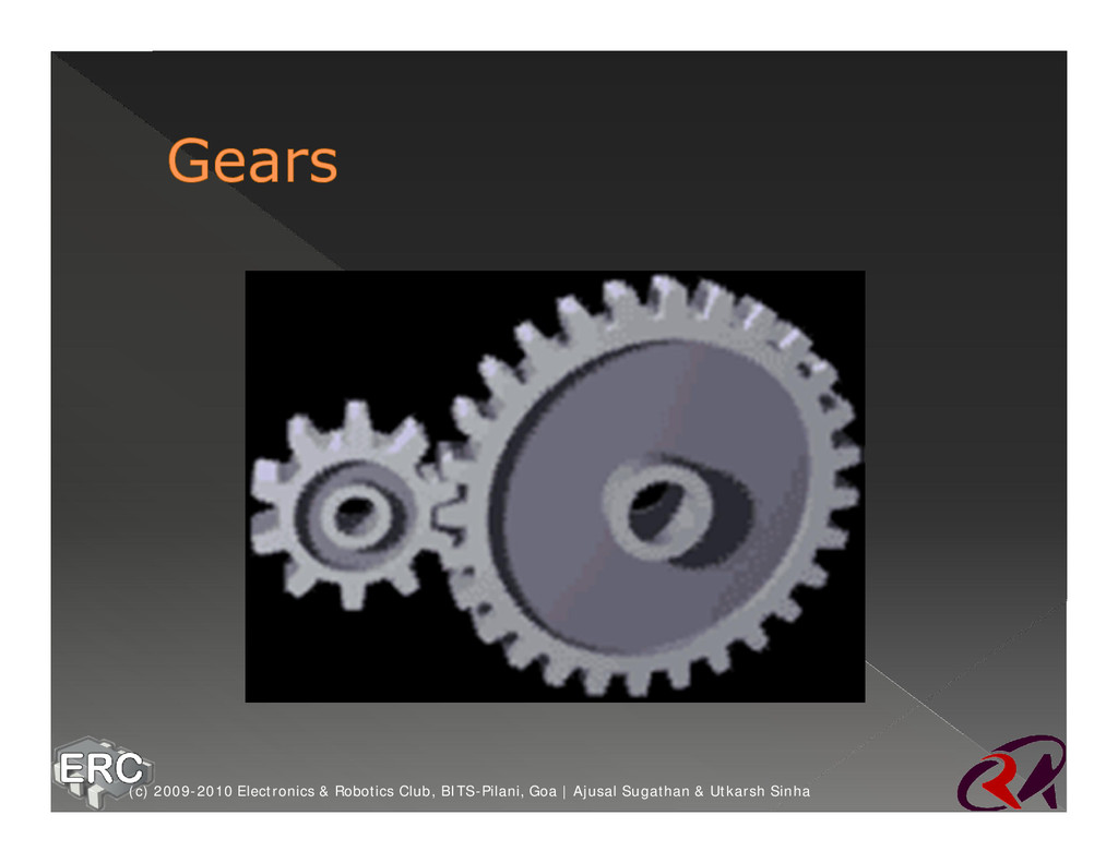
in mechanical engineering Ø Gears form vital elements of mechanisms in many machines such as vehicles, metal tooling machine tools, rolling mills, hoisting etc. Ø In robotics its vital to control actuator speeds and in exercising different degrees of freedom (c) 2009-2010 Electronics & Robotics Club, BITS-Pilani, Goa | Ajusal Sugathan & Utkarsh Sinha
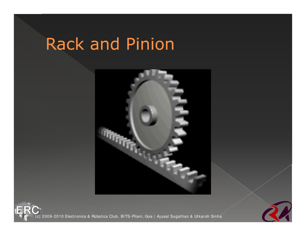
are analogous to transformers in electrical systems Ø It follows the basic equation: Ø ω1 x r1 = ω2 x r2 Ø Gears are very useful in transferring motion between different dimension (c) 2009-2010 Electronics & Robotics Club, BITS-Pilani, Goa | Ajusal Sugathan & Utkarsh Sinha
linear motion Ø Same mechanism used to steer wheels using a steering Ø In robotics used extensively in clamping systems (c) 2009-2010 Electronics & Robotics Club, BITS-Pilani, Goa | Ajusal Sugathan & Utkarsh Sinha
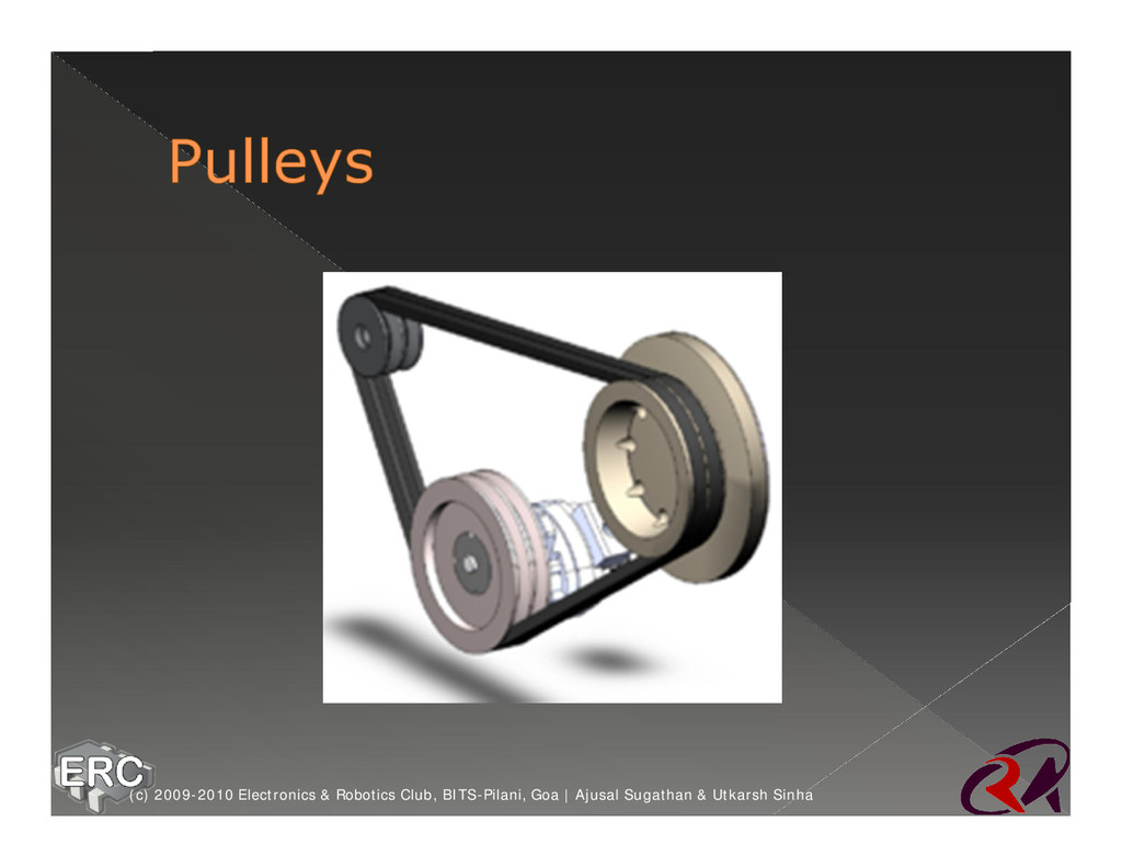
be transmitted across axes Ø If the pulleys are of differing diameters, it gives a mechanical advantage Ø In robotics it can be used in lifting loads or speed reduction Ø Also it can be used in a differential drive to interconnect wheels (c) 2009-2010 Electronics & Robotics Club, BITS-Pilani, Goa | Ajusal Sugathan & Utkarsh Sinha
with a chain Ø It is similar to the system found in bicycles Ø It can transfer rotary motion between shafts in cases where gears are unsuitable Ø Can be used over a larger distance Ø Compared to pulleys has lesser slippage due to firm meshing between the chain and sprocket (c) 2009-2010 Electronics & Robotics Club, BITS-Pilani, Goa | Ajusal Sugathan & Utkarsh Sinha
vHook and pick vClamp and pick vSlide a sheet below and pick vMany other ways vLots of Scope for innovation (c) 2009-2010 Electronics & Robotics Club, BITS-Pilani, Goa | Ajusal Sugathan & Utkarsh Sinha
in all areas of natural science ž It is concerned with extracting data from real-world images ž Differences from computer graphics is that computer graphics makes extensive use of primitives like lines, triangles & points. However no such primitives exist in a real world images. (c) 2009-2010 Electronics & Robotics Club, BITS-Pilani, Goa | Ajusal Sugathan & Utkarsh Sinha
PC or Workstation or Digital Signal Processor for processing ž Software to run on the hardware platform (Matlab, Open CV etc.) ž Image representation to process the image (usually matrix) and provide spatial relationship ž A particular color space is used to represent the image (c) 2009-2010 Electronics & Robotics Club, BITS-Pilani, Goa | Ajusal Sugathan & Utkarsh Sinha
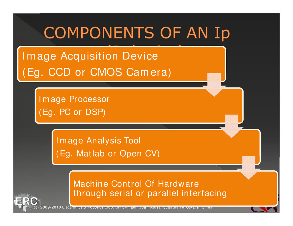
Sugathan & Utkarsh Sinha Image Acquisition Device (Eg. CCD or CMOS Camera) Image Processor (Eg. PC or DSP) Image Analysis Tool (Eg. Matlab or Open CV) Machine Control Of Hardware through serial or parallel interfacing
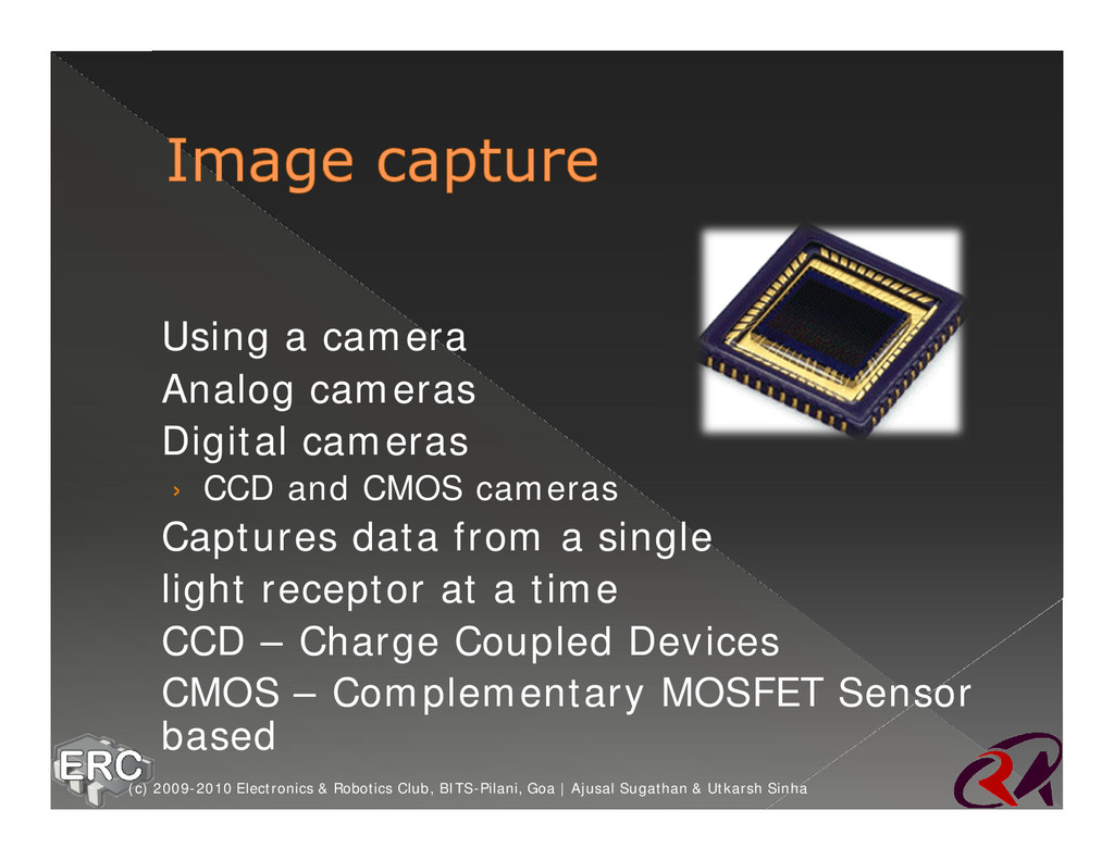
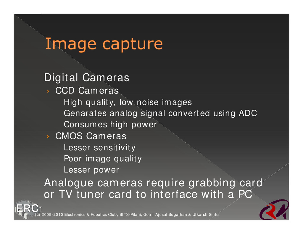
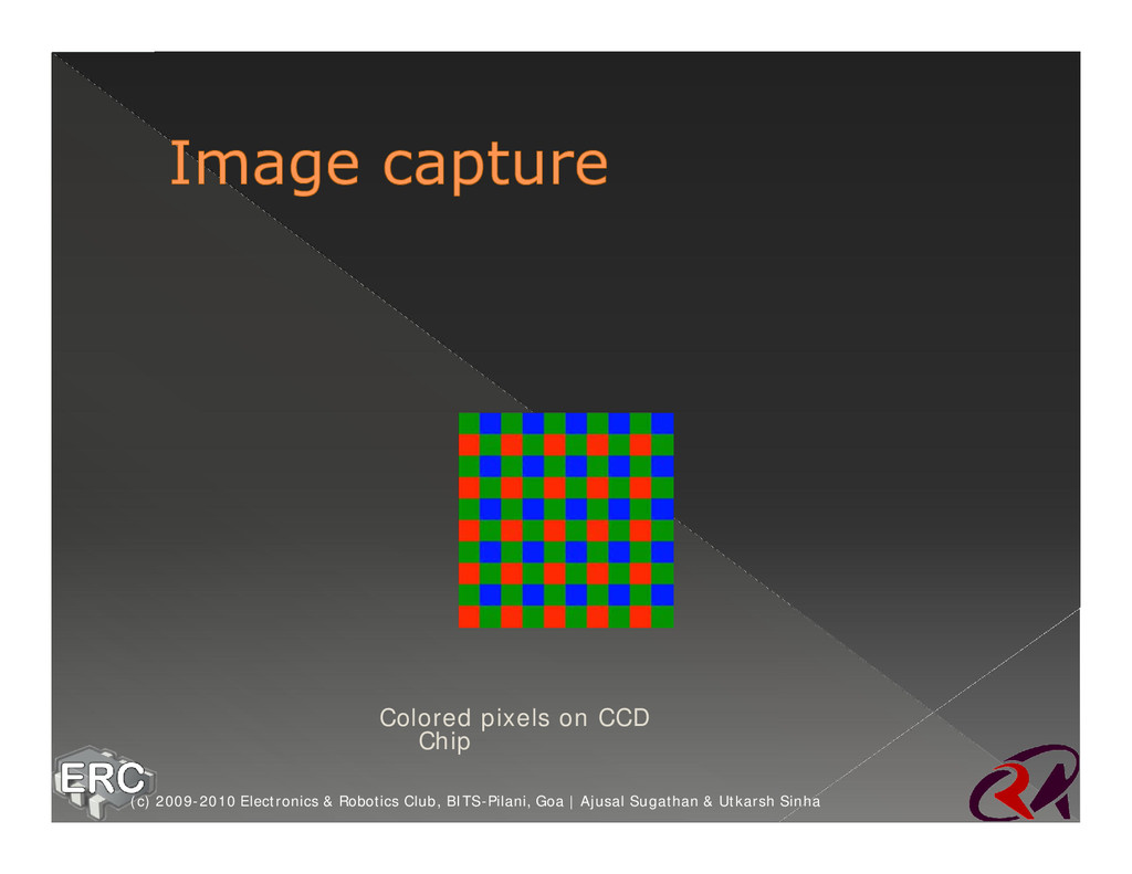
› CCD and CMOS cameras ž Captures data from a single light receptor at a time ž CCD – Charge Coupled Devices ž CMOS – Complementary MOSFET Sensor based (c) 2009-2010 Electronics & Robotics Club, BITS-Pilani, Goa | Ajusal Sugathan & Utkarsh Sinha
noise images – Genarates analog signal converted using ADC – Consumes high power › CMOS Cameras – Lesser sensitivity – Poor image quality – Lesser power ž Analogue cameras require grabbing card or TV tuner card to interface with a PC (c) 2009-2010 Electronics & Robotics Club, BITS-Pilani, Goa | Ajusal Sugathan & Utkarsh Sinha
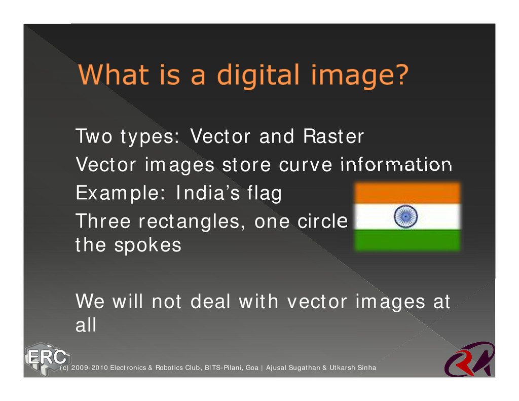
curve information ž Example: India’s flag ž Three rectangles, one circle and the spokes ž We will not deal with vector images at all (c) 2009-2010 Electronics & Robotics Club, BITS-Pilani, Goa | Ajusal Sugathan & Utkarsh Sinha
a raster display ž Also, vector images are high level abstractions ž Vector representations are more complex and used for specific purposes (c) 2009-2010 Electronics & Robotics Club, BITS-Pilani, Goa | Ajusal Sugathan & Utkarsh Sinha
› Pyramid Of the four, matrix is the most general. The other three are used for special purposes. All these representations must provide for spatial relationships (c) 2009-2010 Electronics & Robotics Club, BITS-Pilani, Goa | Ajusal Sugathan & Utkarsh Sinha
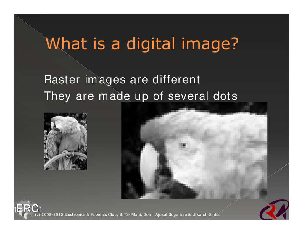
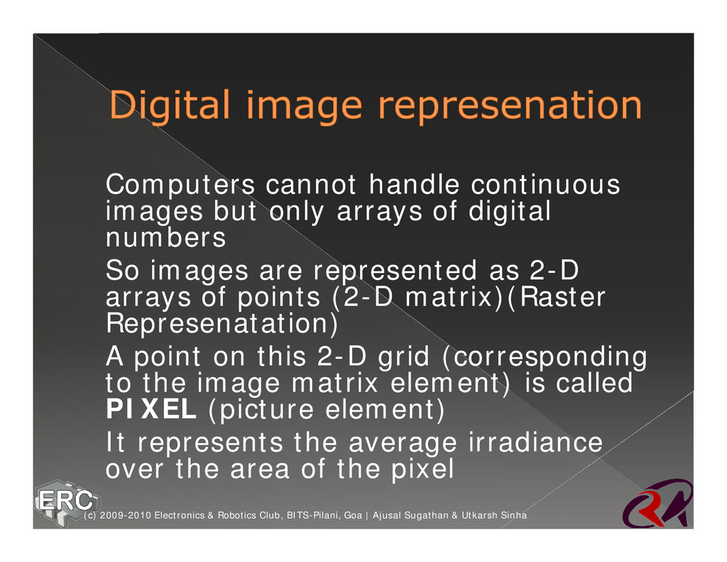
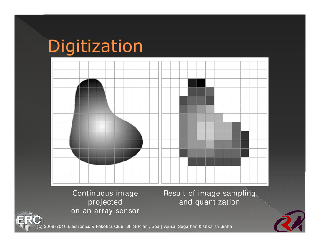
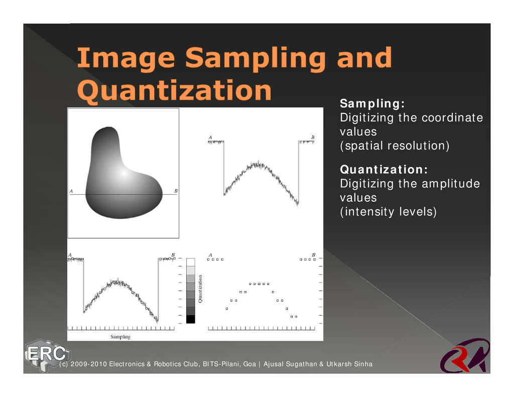
digital numbers ž So images are represented as 2-D arrays of points (2-D matrix)(Raster Represenatation) ž A point on this 2-D grid (corresponding to the image matrix element) is called PIXEL (picture element) ž It represents the average irradiance over the area of the pixel (c) 2009-2010 Electronics & Robotics Club, BITS-Pilani, Goa | Ajusal Sugathan & Utkarsh Sinha
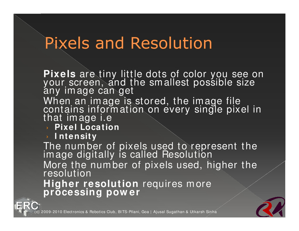
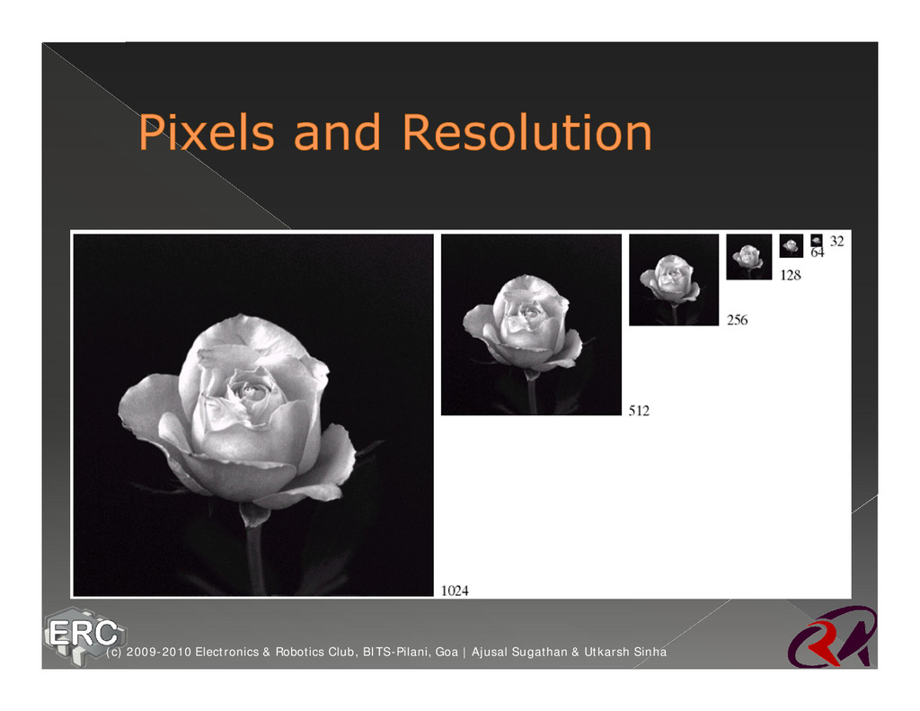
on your screen, and the smallest possible size any image can get ž When an image is stored, the image file contains information on every single pixel in that image i.e › Pixel Location › Intensity ž The number of pixels used to represent the image digitally is called Resolution ž More the number of pixels used, higher the resolution ž Higher resolution requires more processing power (c) 2009-2010 Electronics & Robotics Club, BITS-Pilani, Goa | Ajusal Sugathan & Utkarsh Sinha
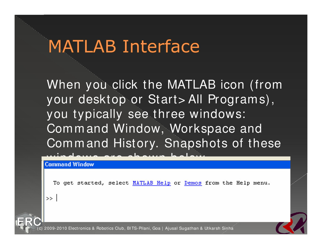
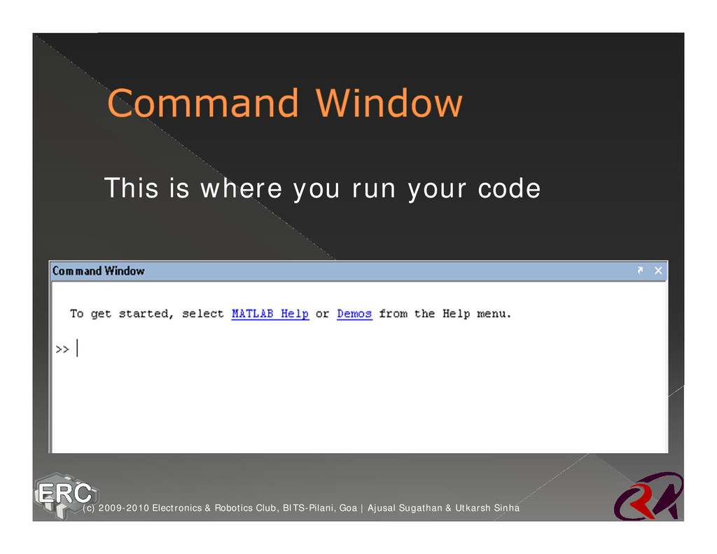
or Start>All Programs), you typically see three windows: Command Window, Workspace and Command History. Snapshots of these windows are shown below (c) 2009-2010 Electronics & Robotics Club, BITS-Pilani, Goa | Ajusal Sugathan & Utkarsh Sinha
which could be either an integer, real numbers or even complex numbers ž These matrices bear some resemblance to array data structures (used in computer programming) (c) 2009-2010 Electronics & Robotics Club, BITS-Pilani, Goa | Ajusal Sugathan & Utkarsh Sinha
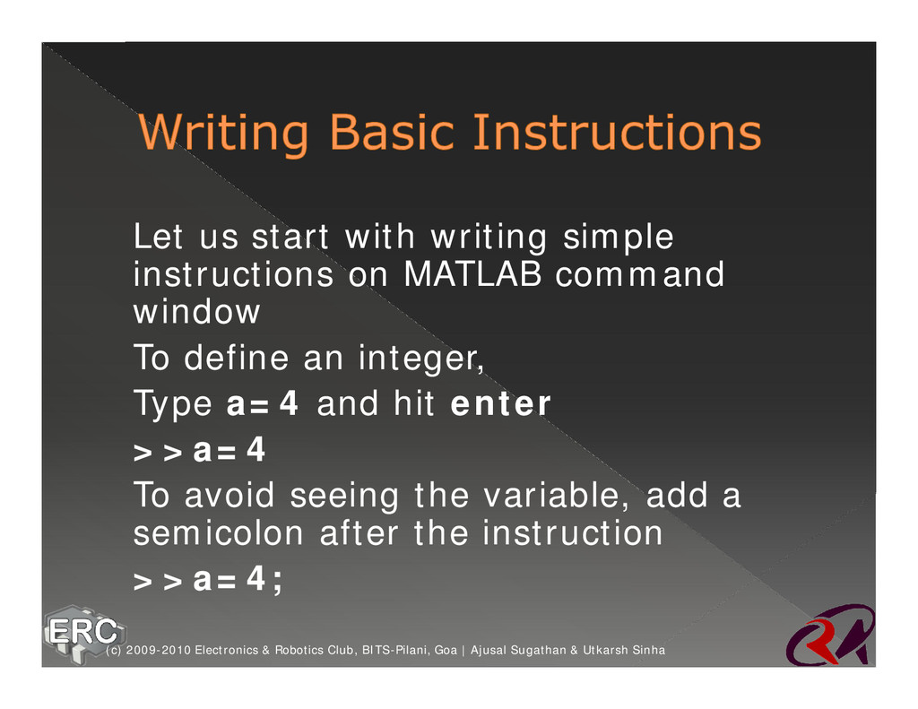
command window ž To define an integer, ž Type a=4 and hit enter ž >>a=4 ž To avoid seeing the variable, add a semicolon after the instruction ž >>a=4; (c) 2009-2010 Electronics & Robotics Club, BITS-Pilani, Goa | Ajusal Sugathan & Utkarsh Sinha
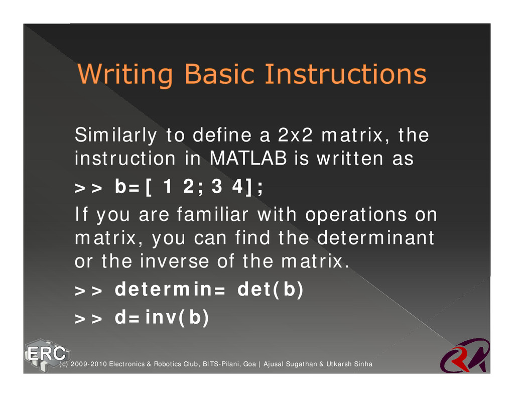
MATLAB is written as ž >> b=[ 1 2; 3 4]; ž If you are familiar with operations on matrix, you can find the determinant or the inverse of the matrix. ž >> determin= det(b) ž >> d=inv(b) (c) 2009-2010 Electronics & Robotics Club, BITS-Pilani, Goa | Ajusal Sugathan & Utkarsh Sinha
matrices ž So now we try to see this for real on MATLAB ž We shall also look into the basic commands provided by MATLAB’s Image Processing Toolbox (c) 2009-2010 Electronics & Robotics Club, BITS-Pilani, Goa | Ajusal Sugathan & Utkarsh Sinha
the Command Window ž >> im=imread(‘sample.jpg'); ž This command stores the file image file ‘sample.jpg’ in a variable called ‘im’ ž It takes this file from the Current- Directory specified ž Else, entire path of file should be mentioned (c) 2009-2010 Electronics & Robotics Club, BITS-Pilani, Goa | Ajusal Sugathan & Utkarsh Sinha
using imshow command ž >>figure,imshow(im); ž This pops up another window (called as figure window), and displays the image ‘im’ (c) 2009-2010 Electronics & Robotics Club, BITS-Pilani, Goa | Ajusal Sugathan & Utkarsh Sinha
toview the image ž imview(im); ž Difference is that in this case you can see specific pixel values just by moving the cursor over the image (c) 2009-2010 Electronics & Robotics Club, BITS-Pilani, Goa | Ajusal Sugathan & Utkarsh Sinha
use the size function, ž >>s=size(im); ž The size function basically gives the size of any array in MATLAB ž Here we get the size of the IMAGE ARRAY (c) 2009-2010 Electronics & Robotics Club, BITS-Pilani, Goa | Ajusal Sugathan & Utkarsh Sinha
variable we can observe and understand the following: ž How pixels are stored? ž What does the values given by each pixel indicate? ž What is Image Resolution? (c) 2009-2010 Electronics & Robotics Club, BITS-Pilani, Goa | Ajusal Sugathan & Utkarsh Sinha
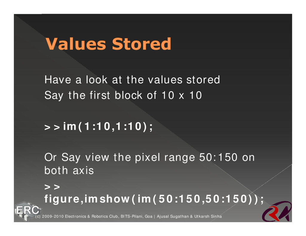
the first block of 10 x 10 ž >>im(1:10,1:10); ž Or Say view the pixel range 50:150 on both axis ž >> figure,imshow(im(50:150,50:150)); (c) 2009-2010 Electronics & Robotics Club, BITS-Pilani, Goa | Ajusal Sugathan & Utkarsh Sinha
different shades ž 24-bit = 224 different shades ž 64-bit images – High end displays ž Used in HDRI, storing extra information per pixel, etc (c) 2009-2010 Electronics & Robotics Club, BITS-Pilani, Goa | Ajusal Sugathan & Utkarsh Sinha
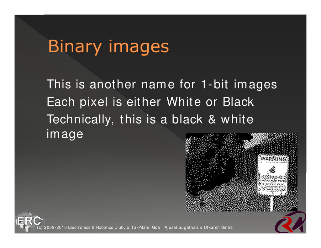
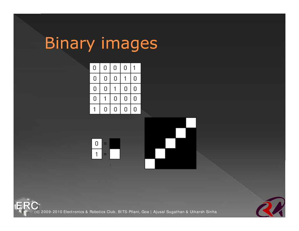
pixel is either White or Black ž Technically, this is a black & white image (c) 2009-2010 Electronics & Robotics Club, BITS-Pilani, Goa | Ajusal Sugathan & Utkarsh Sinha
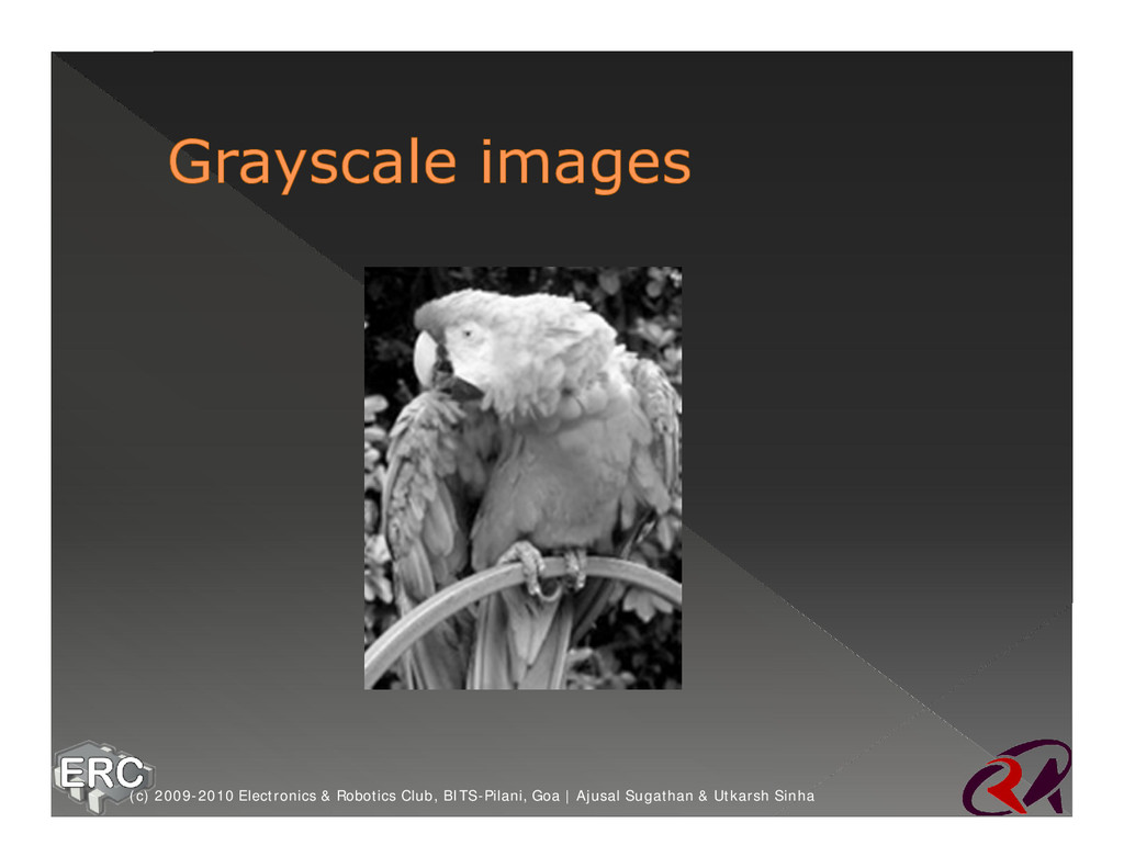
be one of 256 different shades of gray ž These images are popularly called Black & White. Though, this is technically wrong. (c) 2009-2010 Electronics & Robotics Club, BITS-Pilani, Goa | Ajusal Sugathan & Utkarsh Sinha
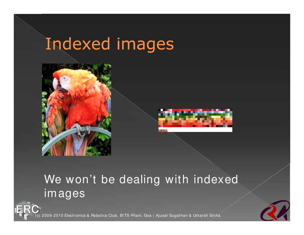
of the 256 values maps to a color in a predefined “palette” ž If required, you can have different bit depths (c) 2009-2010 Electronics & Robotics Club, BITS-Pilani, Goa | Ajusal Sugathan & Utkarsh Sinha
of colors we see ž So 24-bits is generally used for color images ž Thus each pixel can have one of 224 unique colors (c) 2009-2010 Electronics & Robotics Club, BITS-Pilani, Goa | Ajusal Sugathan & Utkarsh Sinha
manage so many different shades? ž Programmers would go nuts ž Then came along the idea of color spaces (c) 2009-2010 Electronics & Robotics Club, BITS-Pilani, Goa | Ajusal Sugathan & Utkarsh Sinha
way to manage millions of colors ž Eliminates memorization, and increases predictability ž Common color spaces: › RGB › HSV › YCrCb or YUV › YIQ (c) 2009-2010 Electronics & Robotics Club, BITS-Pilani, Goa | Ajusal Sugathan & Utkarsh Sinha
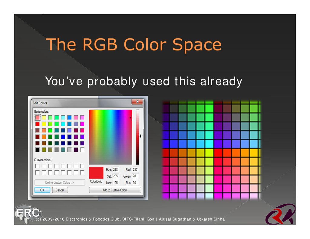
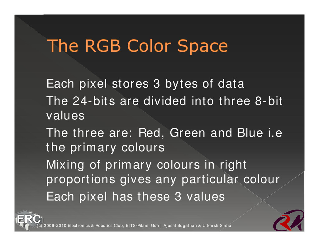
24-bits are divided into three 8-bit values ž The three are: Red, Green and Blue i.e the primary colours ž Mixing of primary colours in right proportions gives any particular colour ž Each pixel has these 3 values (c) 2009-2010 Electronics & Robotics Club, BITS-Pilani, Goa | Ajusal Sugathan & Utkarsh Sinha
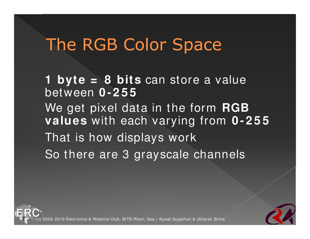
between 0-255 ž We get pixel data in the form RGB values with each varying from 0-255 ž That is how displays work ž So there are 3 grayscale channels (c) 2009-2010 Electronics & Robotics Club, BITS-Pilani, Goa | Ajusal Sugathan & Utkarsh Sinha
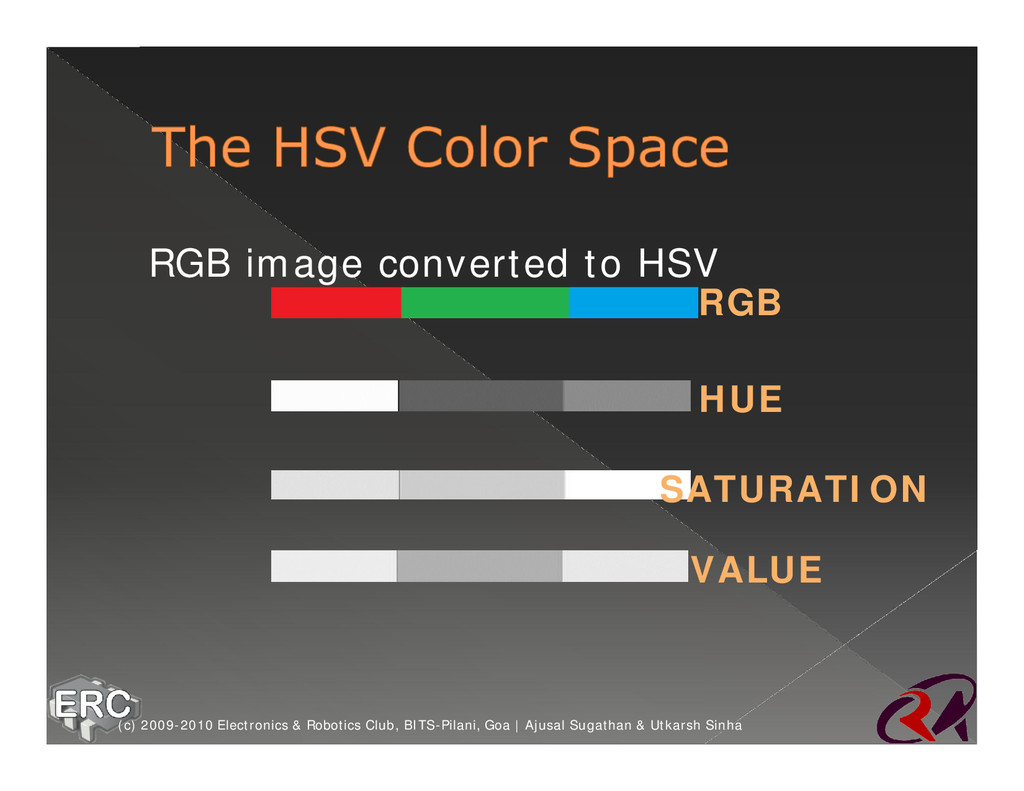
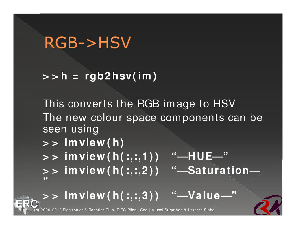
It represents the colour of the pixel (Eg. Red Green Yellow etc) ž The Saturation is the “amount” of that tint › It represents the intensity of the colour (Eg. Dark red and light red) ž The Value is the “intensity” of that pixel › It represents the intensity of brightness of the colour (c) 2009-2010 Electronics & Robotics Club, BITS-Pilani, Goa | Ajusal Sugathan & Utkarsh Sinha
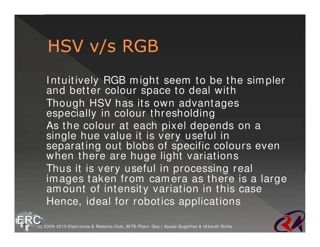
better colour space to deal with ž Though HSV has its own advantages especially in colour thresholding ž As the colour at each pixel depends on a single hue value it is very useful in separating out blobs of specific colours even when there are huge light variations ž Thus it is very useful in processing real images taken from camera as there is a large amount of intensity variation in this case ž Hence, ideal for robotics applications (c) 2009-2010 Electronics & Robotics Club, BITS-Pilani, Goa | Ajusal Sugathan & Utkarsh Sinha
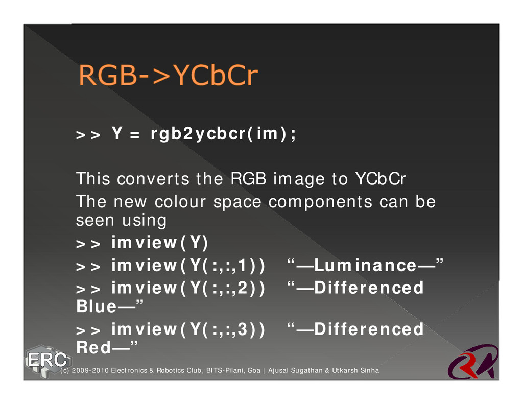
channels: › Y Component: – Gives luminance or intensity › Cr Component: – It is the RED component minus a reference value › Cb Component: – It is the BLUE component minus a reference value ž Hence Cr and Cb components represent the colour called “Color Difference Components” (c) 2009-2010 Electronics & Robotics Club, BITS-Pilani, Goa | Ajusal Sugathan & Utkarsh Sinha
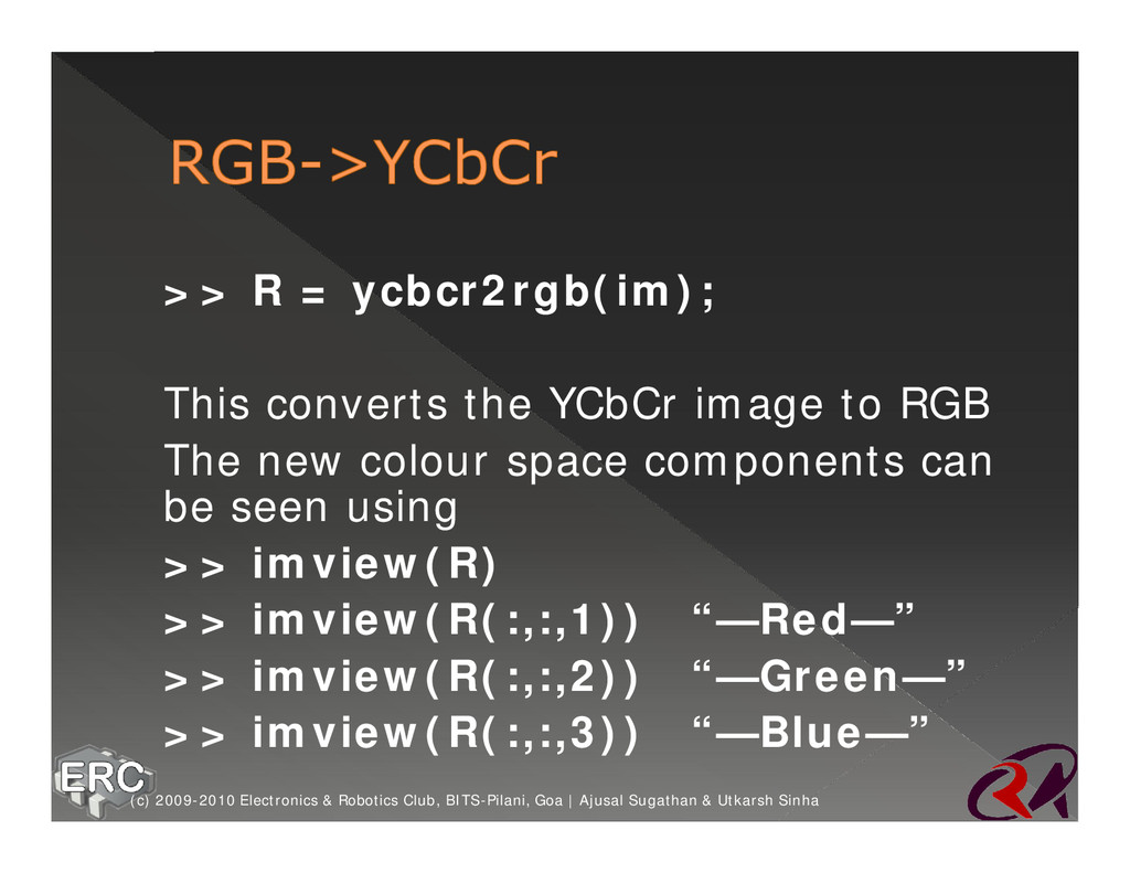
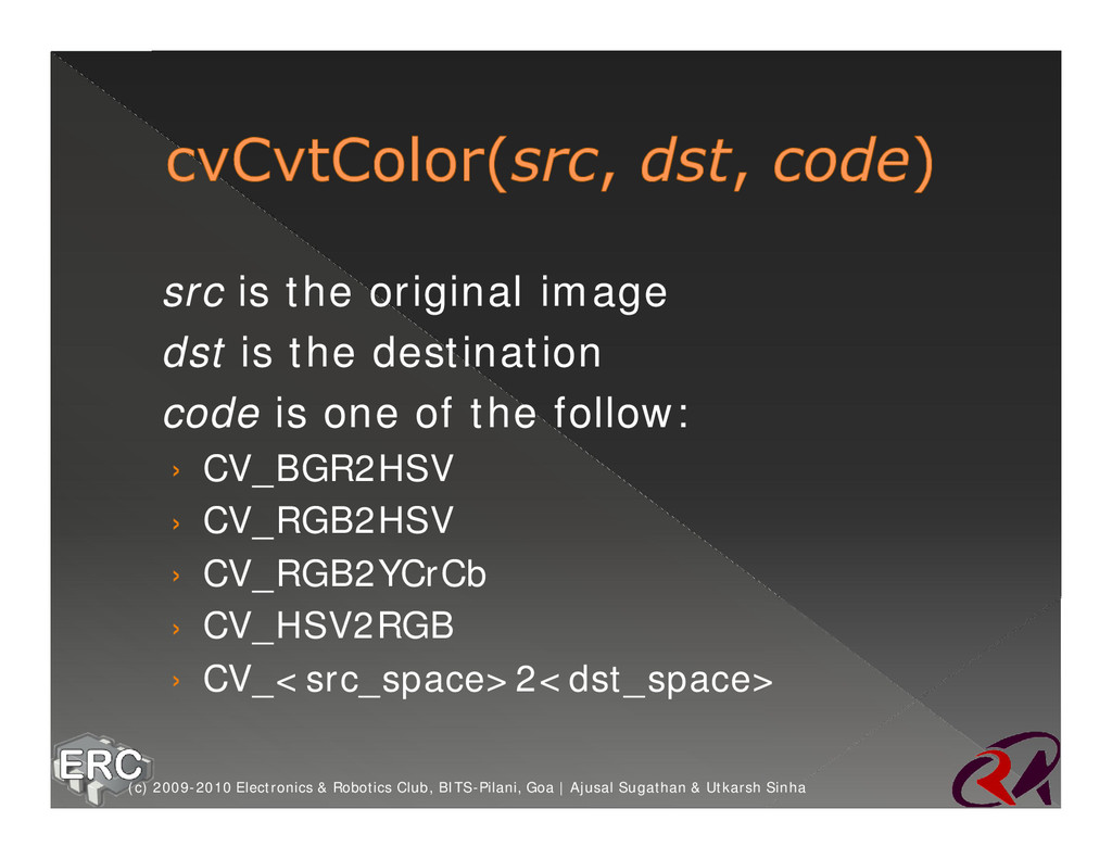
ž You might want to convert to different color spaces to process it ž Colour space conversions can take place between RGB to any other colour space and vice versa (c) 2009-2010 Electronics & Robotics Club, BITS-Pilani, Goa | Ajusal Sugathan & Utkarsh Sinha
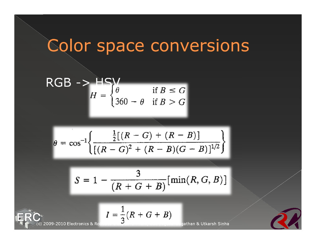
best thing is, you don’t need to remember these formulae ž Matlab and OpenCV have built-in functions for these transformations :-) (c) 2009-2010 Electronics & Robotics Club, BITS-Pilani, Goa | Ajusal Sugathan & Utkarsh Sinha
in image processing ž You can use OpenCV in C/C++, .net languages, Java, Python, etc as well ž We will only discuss OpenCV in C/C++ (c) 2009-2010 Electronics & Robotics Club, BITS-Pilani, Goa | Ajusal Sugathan & Utkarsh Sinha
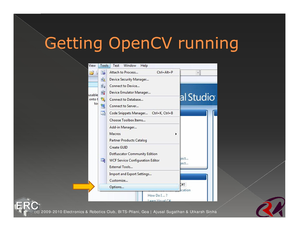
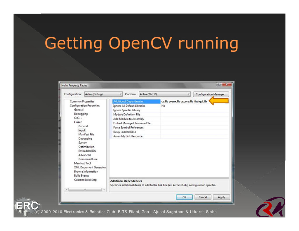
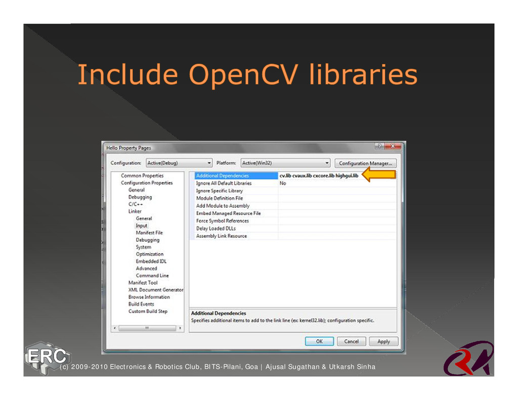
we’ve installed OpenCV ž So, we tell it where to find the OpenCV header files ž Start Microsoft Visual Studio 2008 (c) 2009-2010 Electronics & Robotics Club, BITS-Pilani, Goa | Ajusal Sugathan & Utkarsh Sinha
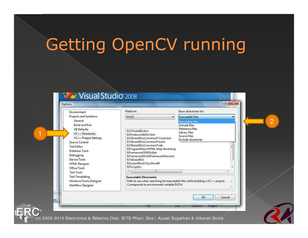
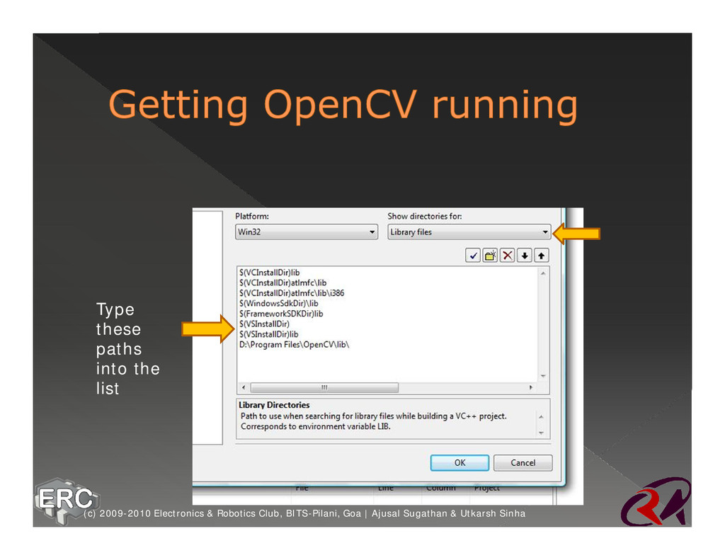
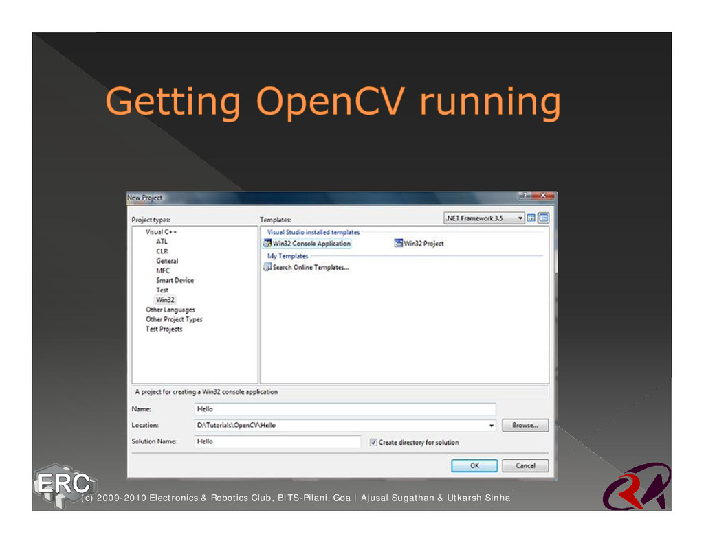
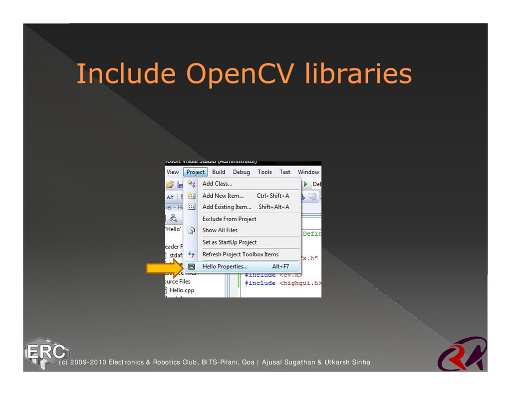
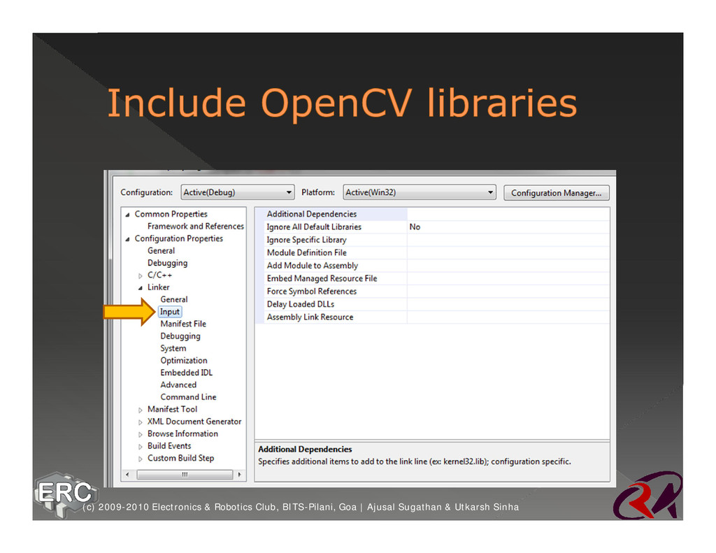
OpenCV include files and library files ž Now we create a new project (c) 2009-2010 Electronics & Robotics Club, BITS-Pilani, Goa | Ajusal Sugathan & Utkarsh Sinha
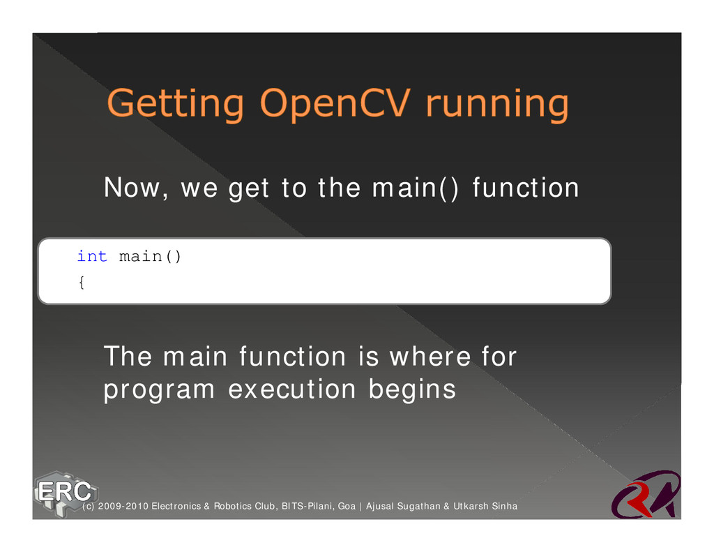
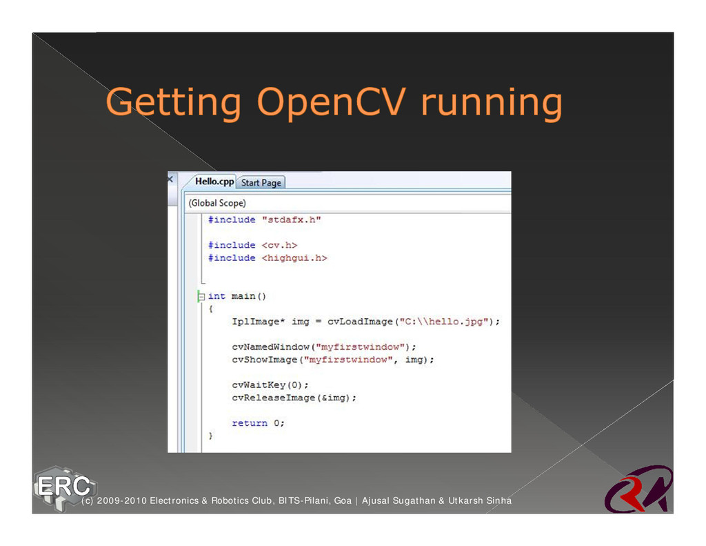
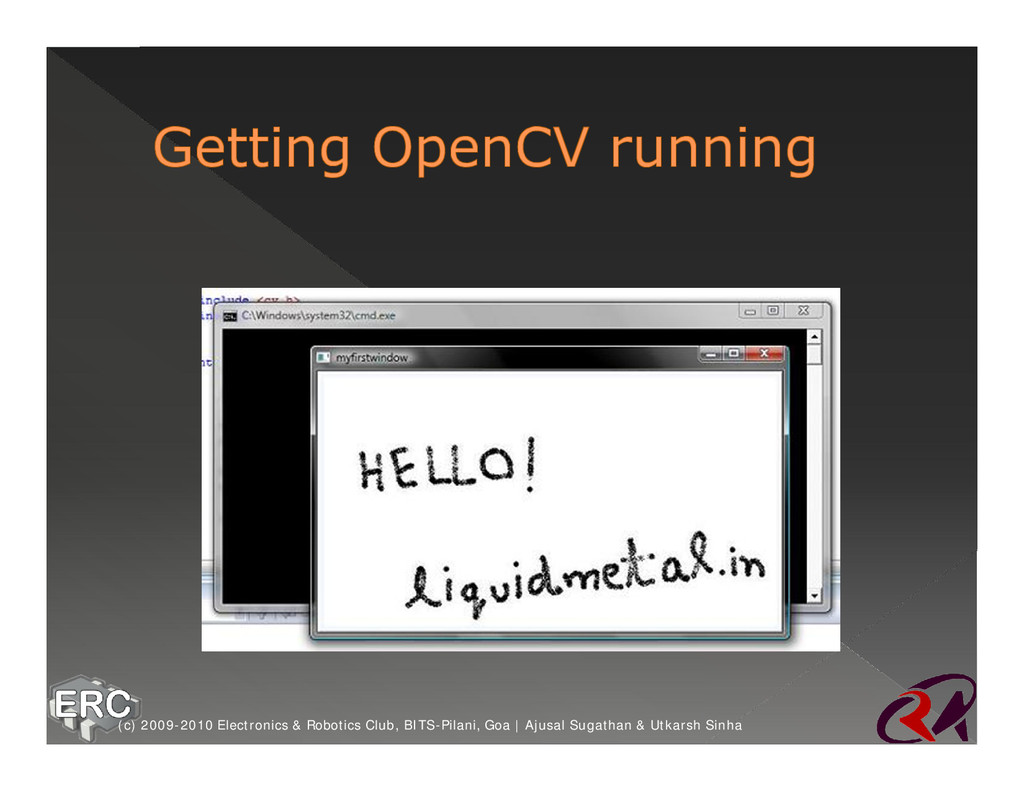
end up with an empty project with a single file (like Mybot.cpp) ž Open this file, we’ll write some code now (c) 2009-2010 Electronics & Robotics Club, BITS-Pilani, Goa | Ajusal Sugathan & Utkarsh Sinha
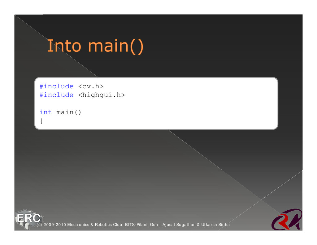
{ ž The main function is where for program execution begins (c) 2009-2010 Electronics & Robotics Club, BITS-Pilani, Goa | Ajusal Sugathan & Utkarsh Sinha
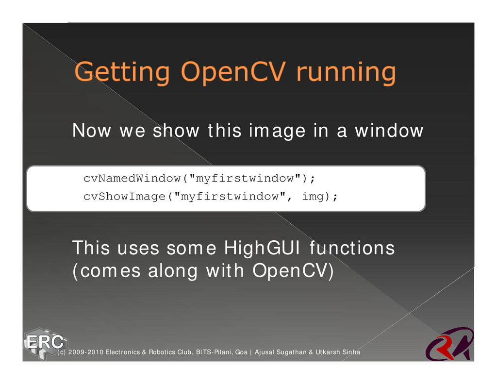
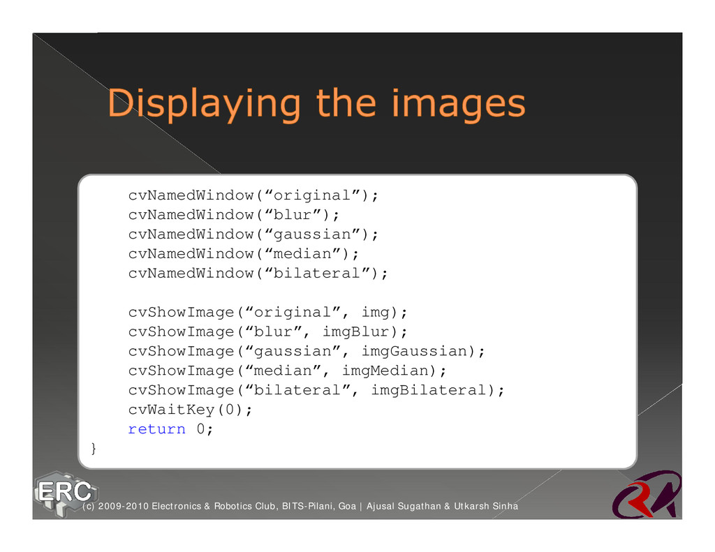
is a HighGUI function ž You can add controls to each window as well (track bars, buttons, etc) (c) 2009-2010 Electronics & Robotics Club, BITS-Pilani, Goa | Ajusal Sugathan & Utkarsh Sinha
pressed ž If time=0, waits till eternity ž Here, we’ve used it to keep the windows from vanishing immediately (c) 2009-2010 Electronics & Robotics Club, BITS-Pilani, Goa | Ajusal Sugathan & Utkarsh Sinha
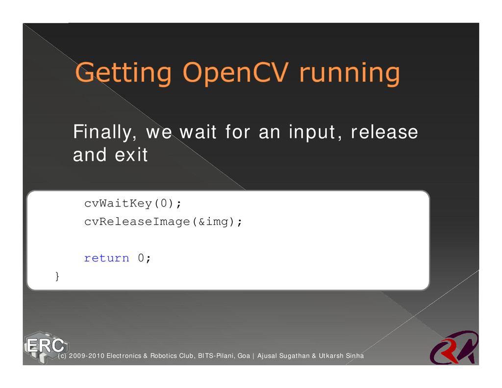
an image as soon as possible. RAM is precious J ž Note that you send the address of the image (&img) and not just the image (img) (c) 2009-2010 Electronics & Robotics Club, BITS-Pilani, Goa | Ajusal Sugathan & Utkarsh Sinha
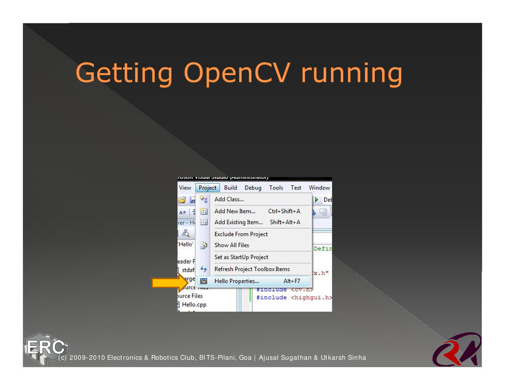
But it does not know, whether to use OpenCV or not ž We need to tell this explicitly (c) 2009-2010 Electronics & Robotics Club, BITS-Pilani, Goa | Ajusal Sugathan & Utkarsh Sinha
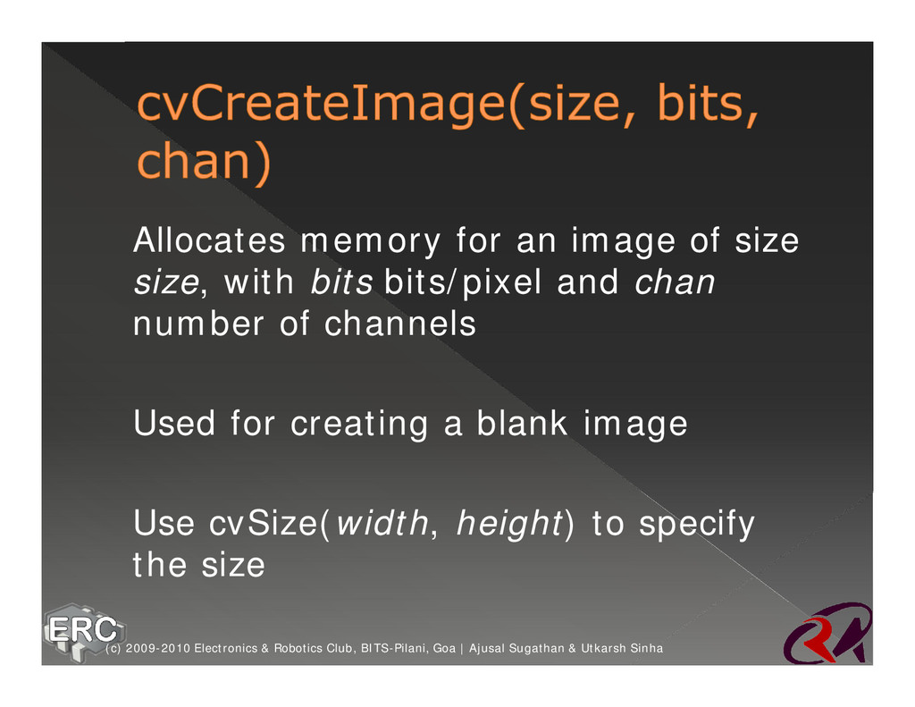
will pop up ž dst should be a valid image, i.e. you need a blank image of the same size ž code should be valid (check the OpenCV documentation for that) (c) 2009-2010 Electronics & Robotics Club, BITS-Pilani, Goa | Ajusal Sugathan & Utkarsh Sinha
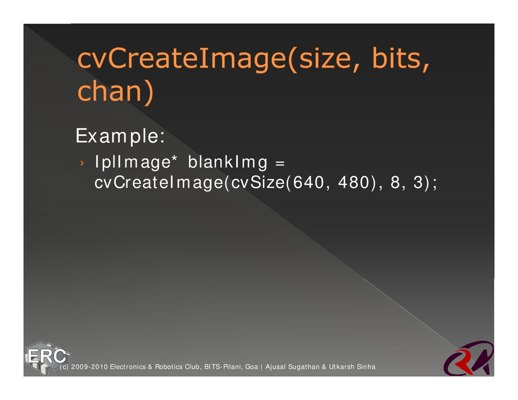
bits bits/pixel and chan number of channels ž Used for creating a blank image ž Use cvSize(width, height) to specify the size (c) 2009-2010 Electronics & Robotics Club, BITS-Pilani, Goa | Ajusal Sugathan & Utkarsh Sinha
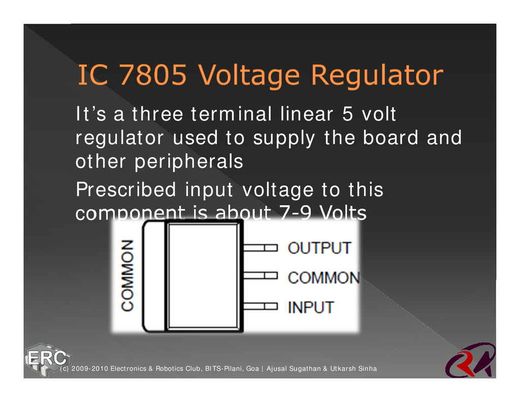
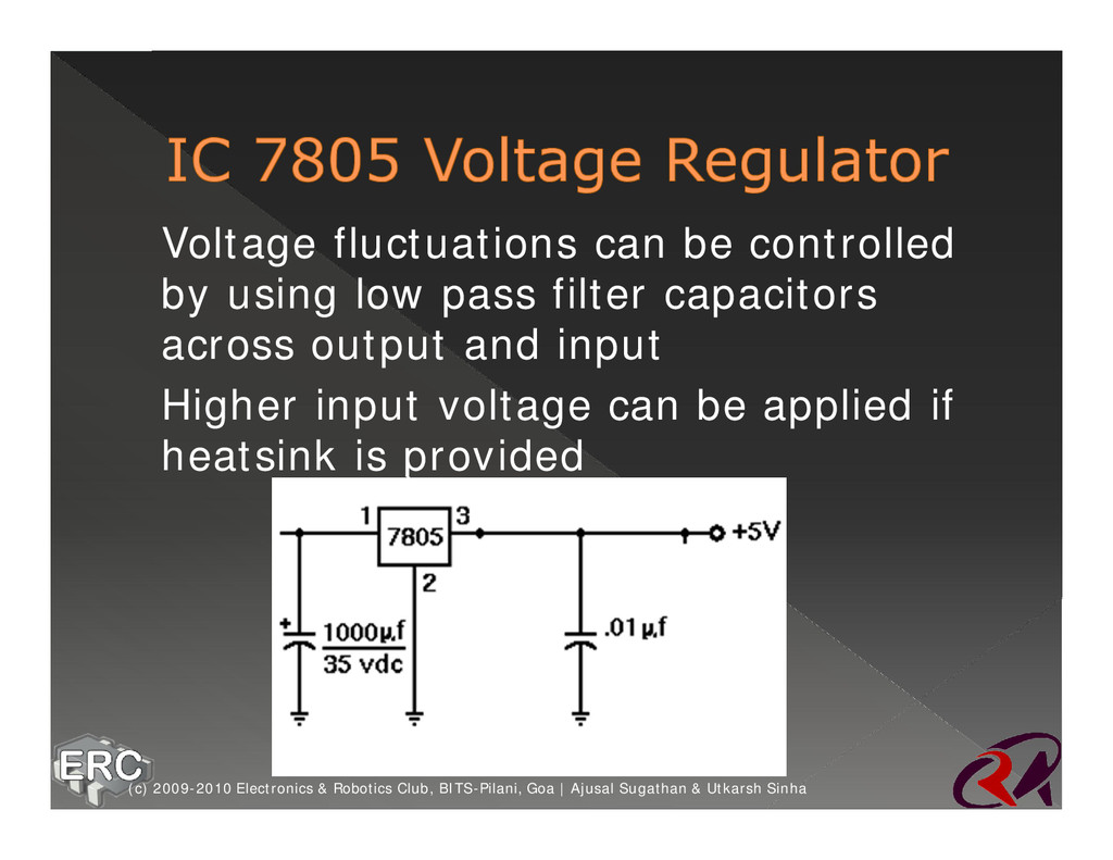
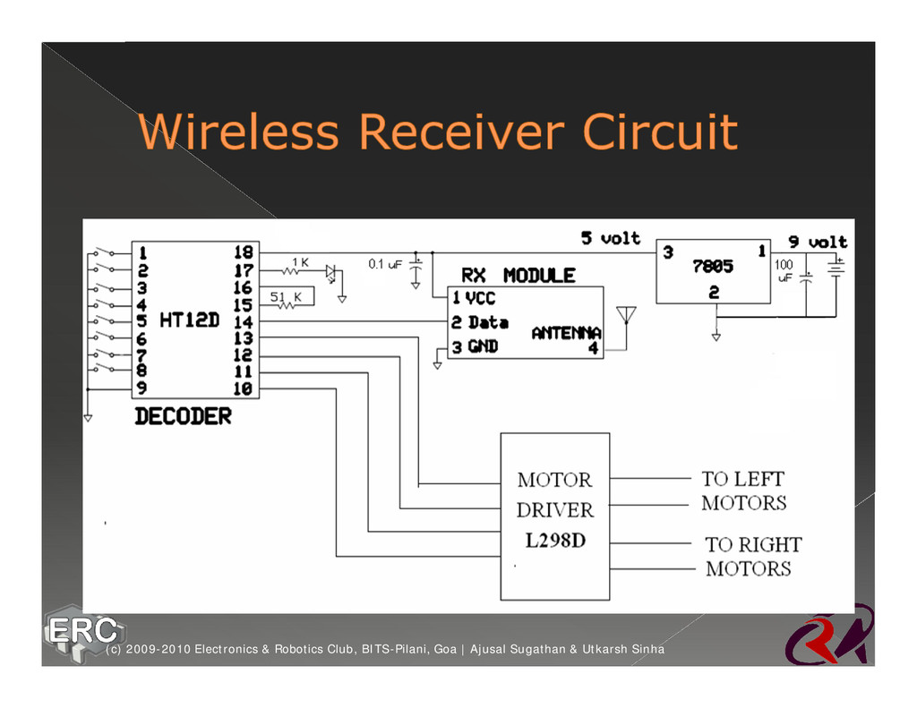
to supply the board and other peripherals ž Prescribed input voltage to this component is about 7-9 Volts (c) 2009-2010 Electronics & Robotics Club, BITS-Pilani, Goa | Ajusal Sugathan & Utkarsh Sinha
filter capacitors across output and input ž Higher input voltage can be applied if heatsink is provided (c) 2009-2010 Electronics & Robotics Club, BITS-Pilani, Goa | Ajusal Sugathan & Utkarsh Sinha
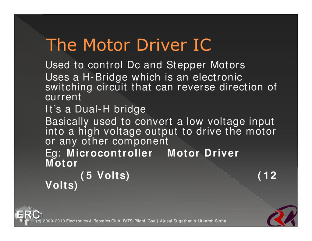
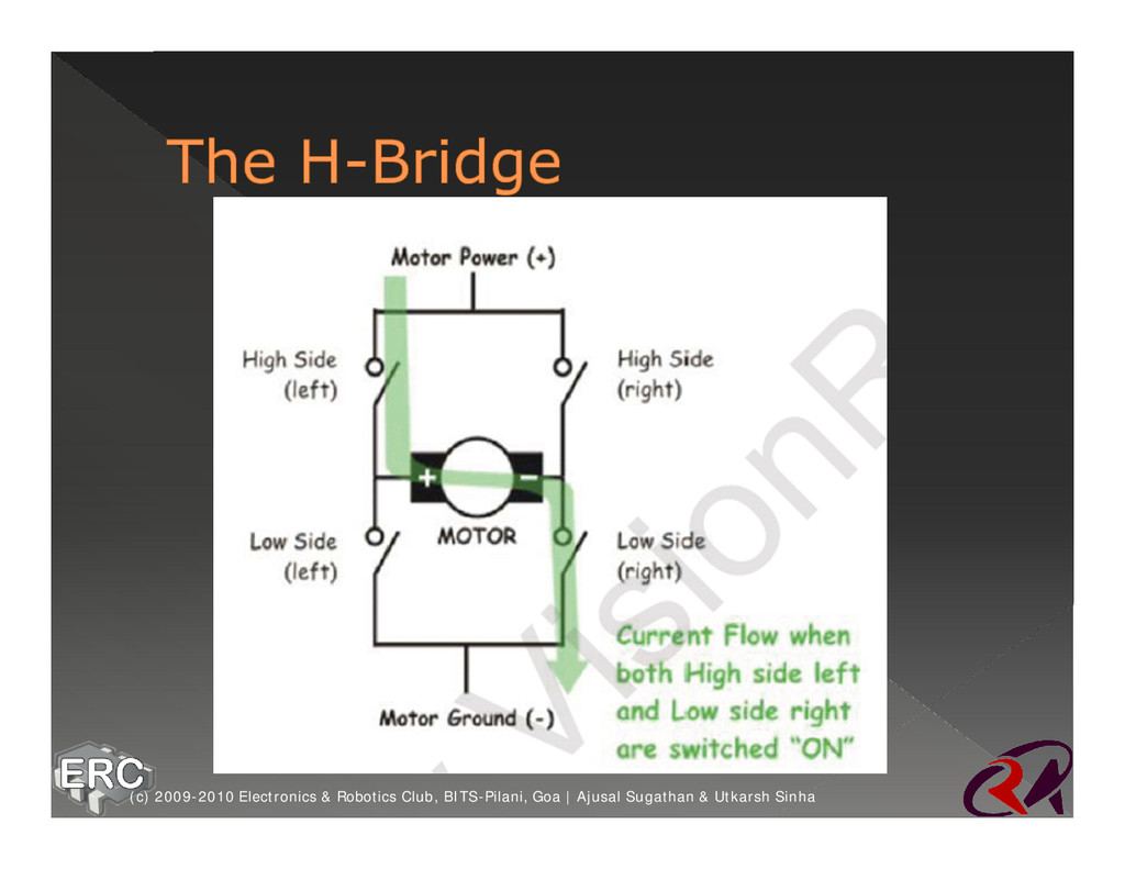
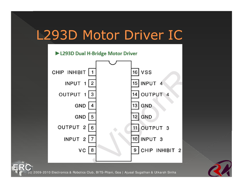
a H-Bridge which is an electronic switching circuit that can reverse direction of current ž It’s a Dual-H bridge ž Basically used to convert a low voltage input into a high voltage output to drive the motor or any other component ž Eg: Microcontrollerà Motor Driverà Motor (5 Volts) (12 Volts) (c) 2009-2010 Electronics & Robotics Club, BITS-Pilani, Goa | Ajusal Sugathan & Utkarsh Sinha
Sugathan & Utkarsh Sinha ž There are many situations where signals and data need to be transferred from one subsystem to another within a piece of electronics ž Relays are too bulky as they are electromechanical in nature and at the same time give lesser efficiency ž In these cases an electronic component called Optocoupler is used
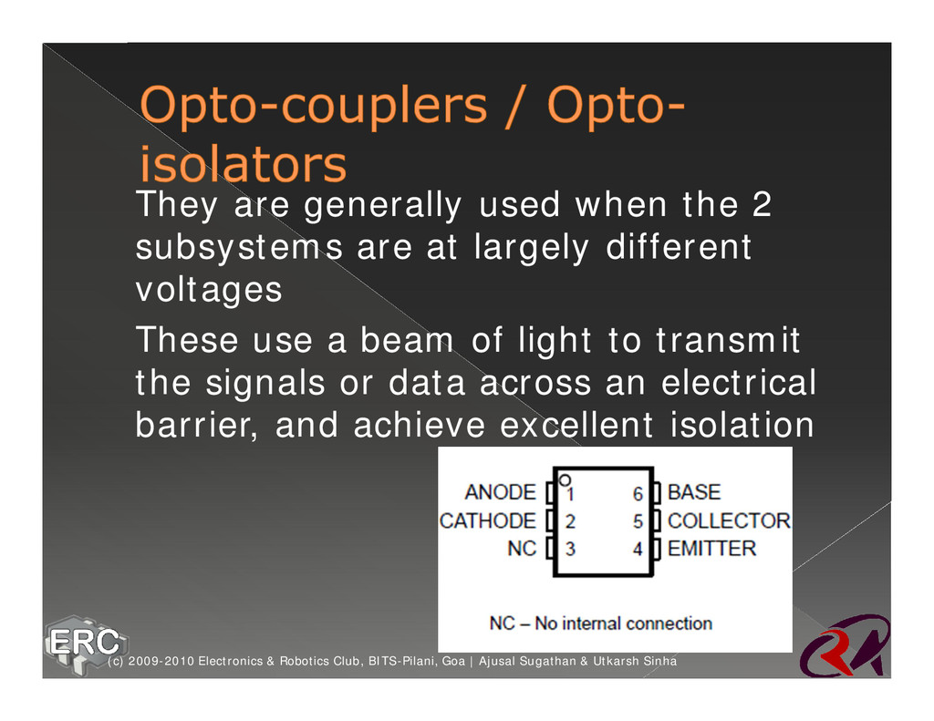
Sugathan & Utkarsh Sinha ž They are generally used when the 2 subsystems are at largely different voltages ž These use a beam of light to transmit the signals or data across an electrical barrier, and achieve excellent isolation
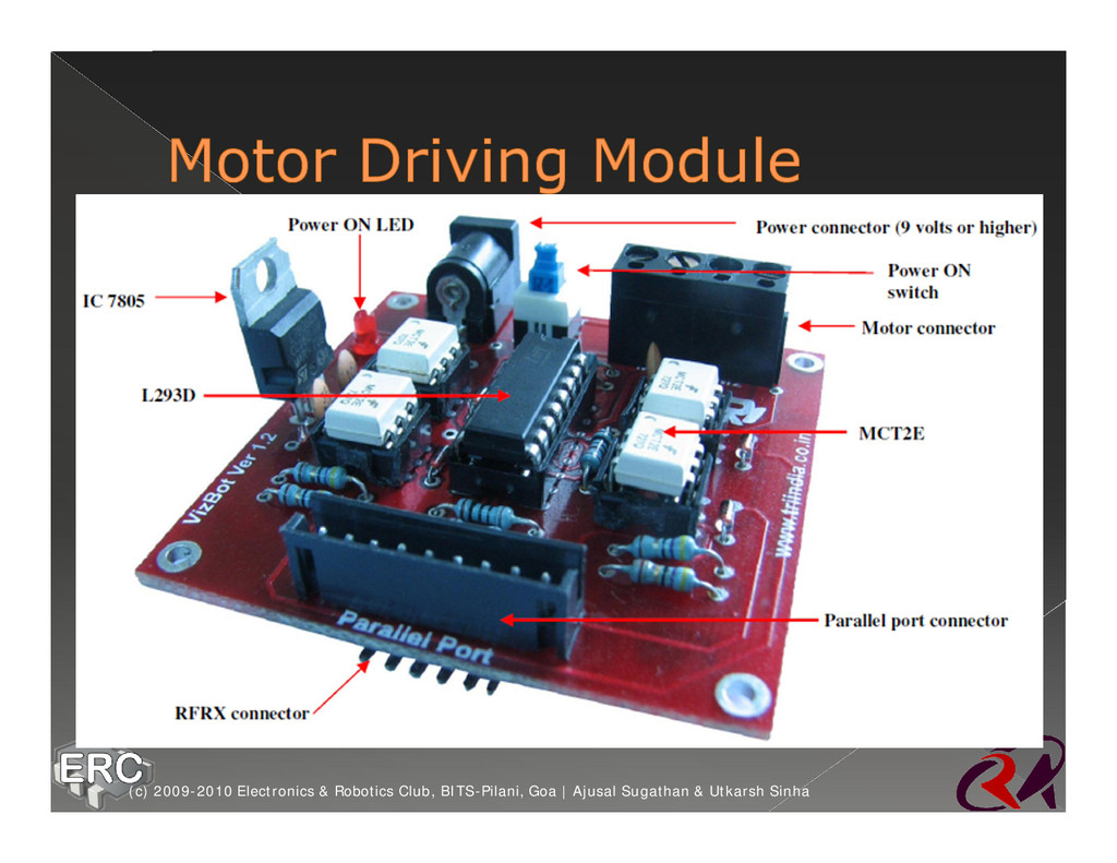
Sugathan & Utkarsh Sinha ž In our circuit, Opto-isolator (MCT2E) is used to ensure electrical isolation between motors and the PC parallel port during wired connection ž The Viz-Board has four such chips to isolate the four data lines (pin 2, pin 3, pin 4, pin 5) coming out of the parallel port
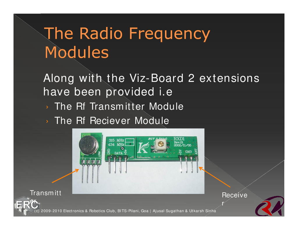
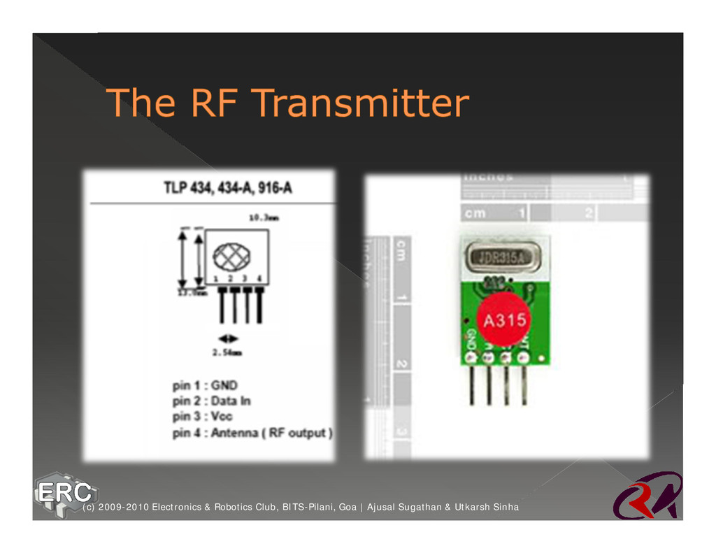
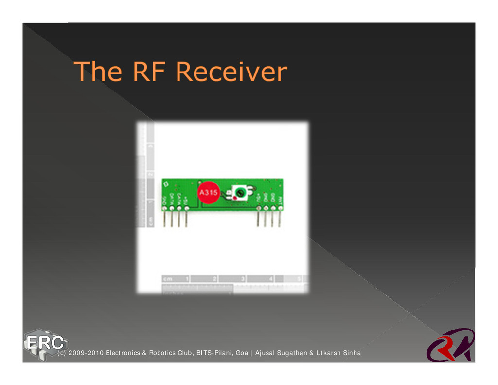
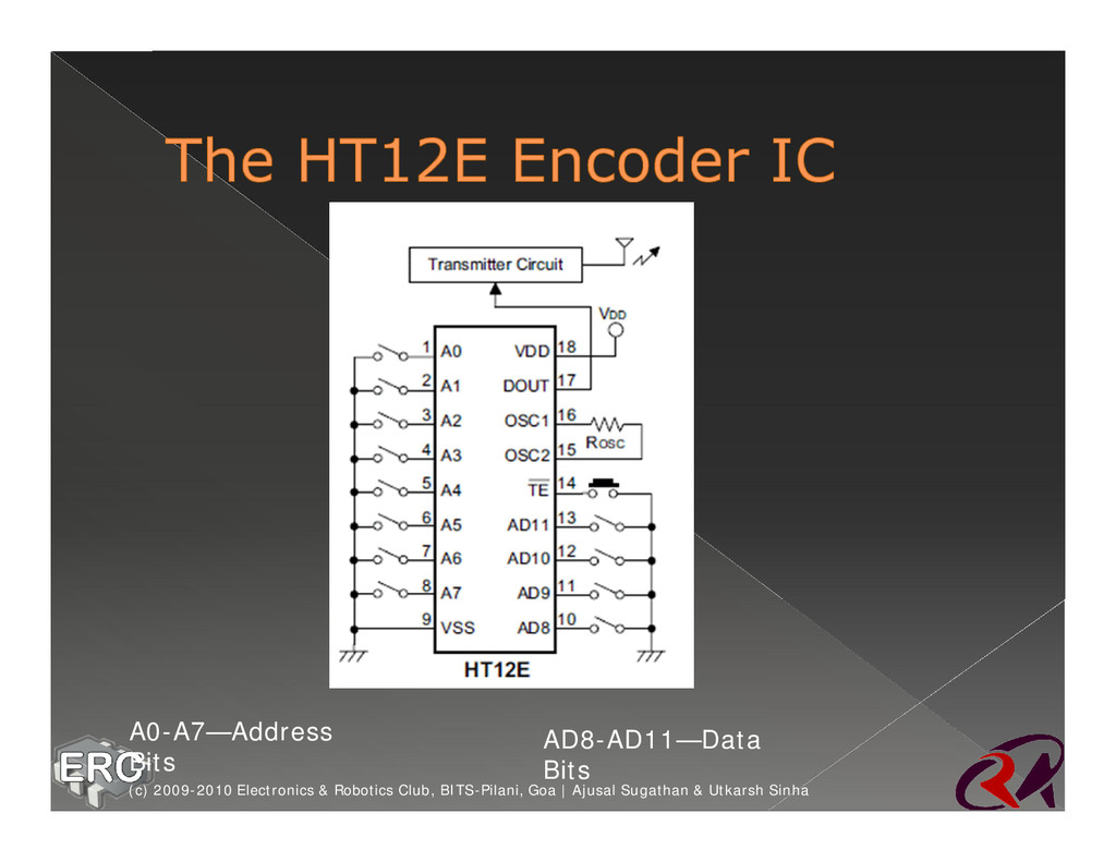
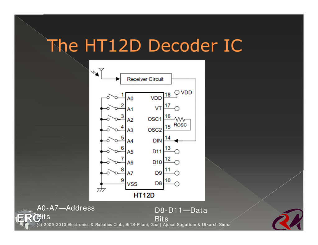
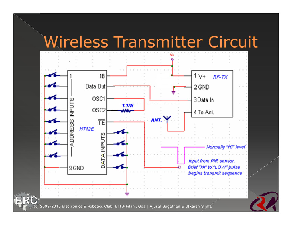
at a certain frequency ž It sends and receives radio waves of a particular frequency and a decoder and encoder IC is provided to encode and decode this information ž Wireless transmission takes place at a particular frequency Eg. 315Mhz ž Theses modules might be single or dual frequency (c) 2009-2010 Electronics & Robotics Club, BITS-Pilani, Goa | Ajusal Sugathan & Utkarsh Sinha
connect any piece of 23 cm long to the Antenna pin ž The kit has a dual frequency RF module with frequencies 315/434 Mhz (c) 2009-2010 Electronics & Robotics Club, BITS-Pilani, Goa | Ajusal Sugathan & Utkarsh Sinha
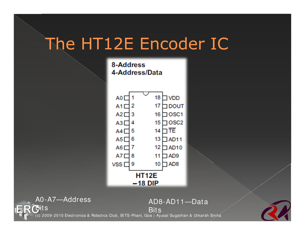
sends it to the RF transmitter module for wireless transmission ž They are capable of encoding information which consists of N address bits and (12-N) data bits (c) 2009-2010 Electronics & Robotics Club, BITS-Pilani, Goa | Ajusal Sugathan & Utkarsh Sinha
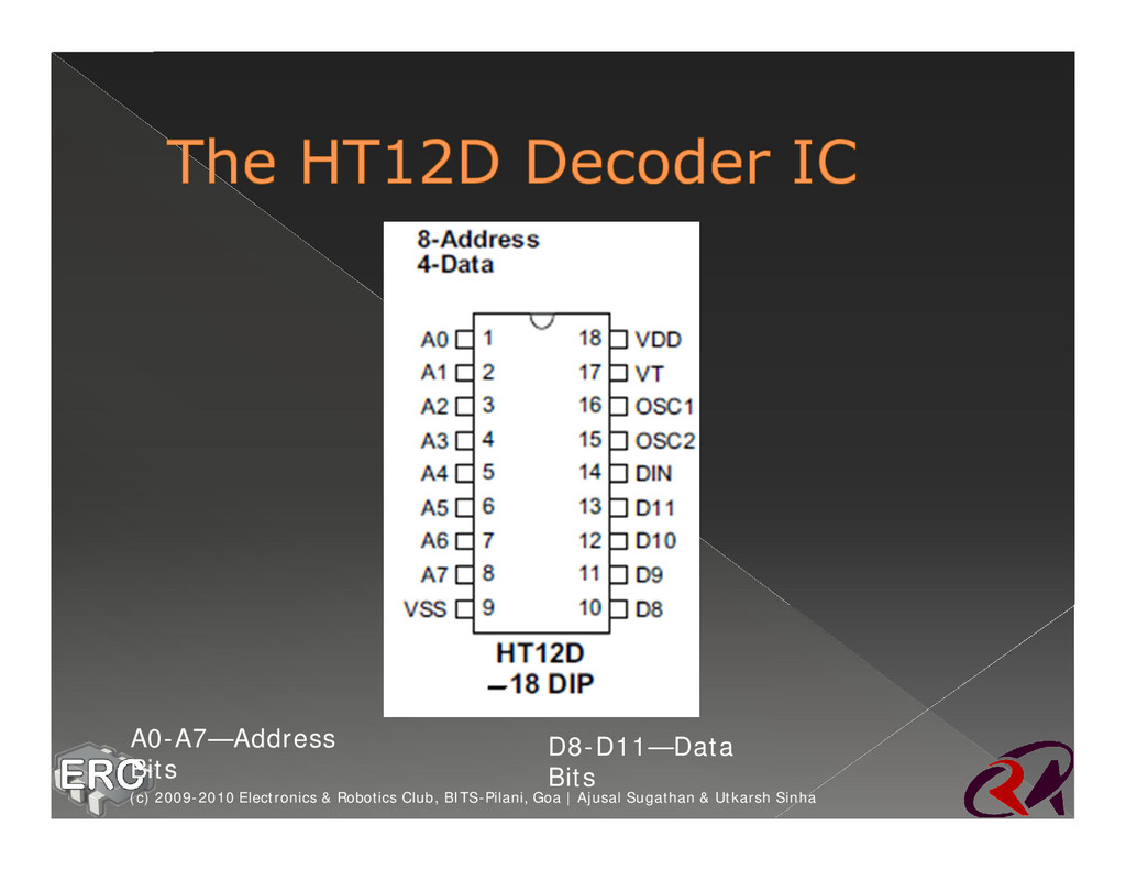
4 data bits ž A DIP-Switch can be used to set or unset the address bits A0-A7 (c) 2009-2010 Electronics & Robotics Club, BITS-Pilani, Goa | Ajusal Sugathan & Utkarsh Sinha
sends it to the parallel port for wireless transmission ž They are capable of encoding information which consists of N address bits and (12-N) data bits (c) 2009-2010 Electronics & Robotics Club, BITS-Pilani, Goa | Ajusal Sugathan & Utkarsh Sinha
4 data bits ž A DIP-Switch can be used to set or unset the address bits A0-A7 (c) 2009-2010 Electronics & Robotics Club, BITS-Pilani, Goa | Ajusal Sugathan & Utkarsh Sinha
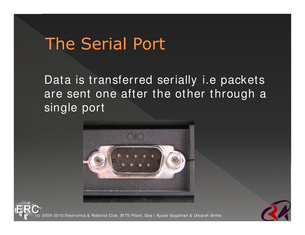
at the same time ž Communication is pretty fast ž Found in old printer ports (c) 2009-2010 Electronics & Robotics Club, BITS-Pilani, Goa | Ajusal Sugathan & Utkarsh Sinha
of data can be transmitted at the same time through parallel ports ž Though parallel and serial ports are not found these days in laptops ž Desktops and old laptops have these ports (c) 2009-2010 Electronics & Robotics Club, BITS-Pilani, Goa | Ajusal Sugathan & Utkarsh Sinha
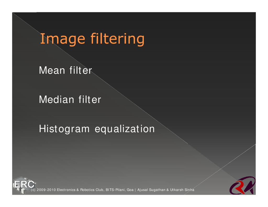
on the image! ž Noise can be reduced by › Using hardware › Using software: filters (c) 2009-2010 Electronics & Robotics Club, BITS-Pilani, Goa | Ajusal Sugathan & Utkarsh Sinha
Due to different factors like changing lighting and other real-time effects ž To improve quality of a captured image to make it easier to process the image (c) 2009-2010 Electronics & Robotics Club, BITS-Pilani, Goa | Ajusal Sugathan & Utkarsh Sinha
remove noise in the input image ž To remove motion blur from an image ž Enhancing the edges of an image to make it appear sharper (c) 2009-2010 Electronics & Robotics Club, BITS-Pilani, Goa | Ajusal Sugathan & Utkarsh Sinha
by taking average over a number of images ž It eliminates noise by assuming that different snaps of the same image have different noise patterns (c) 2009-2010 Electronics & Robotics Club, BITS-Pilani, Goa | Ajusal Sugathan & Utkarsh Sinha
photographs ž The images are extremely faint, and there is more noise than the image itself ž Millions of pictures are taken, and averaged to get a clear picture (c) 2009-2010 Electronics & Robotics Club, BITS-Pilani, Goa | Ajusal Sugathan & Utkarsh Sinha
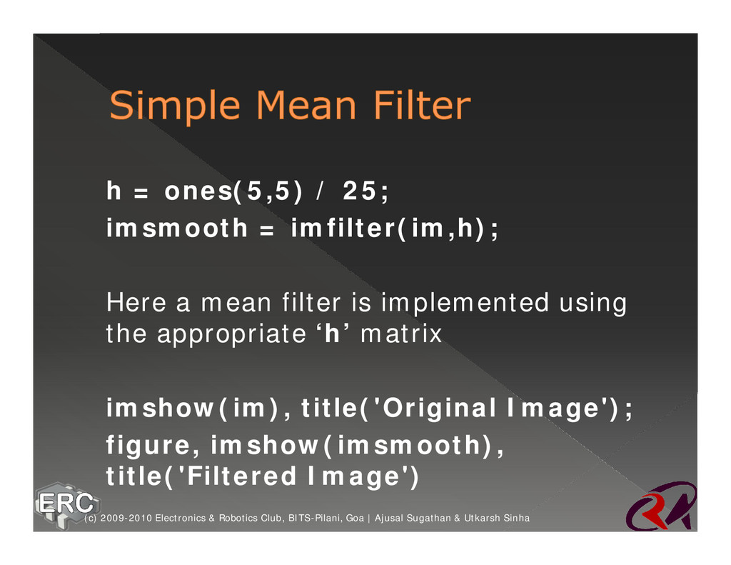
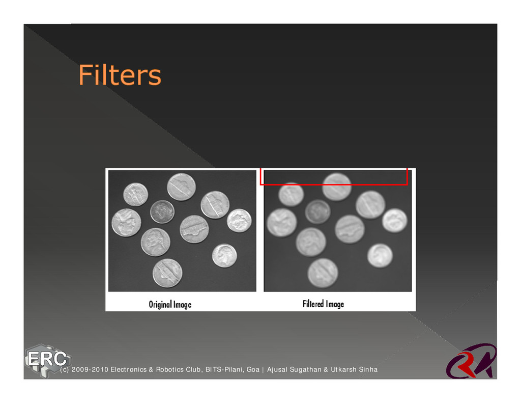
92 as that is the mean value of all surrounding pixels ž This filter is often used to smooth images prior to processing ž It can be used to reduce pixel flicker due to overhead fluorescent lights (c) 2009-2010 Electronics & Robotics Club, BITS-Pilani, Goa | Ajusal Sugathan & Utkarsh Sinha
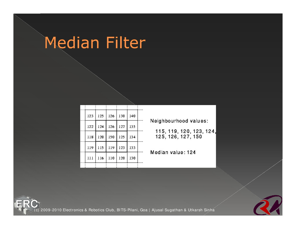
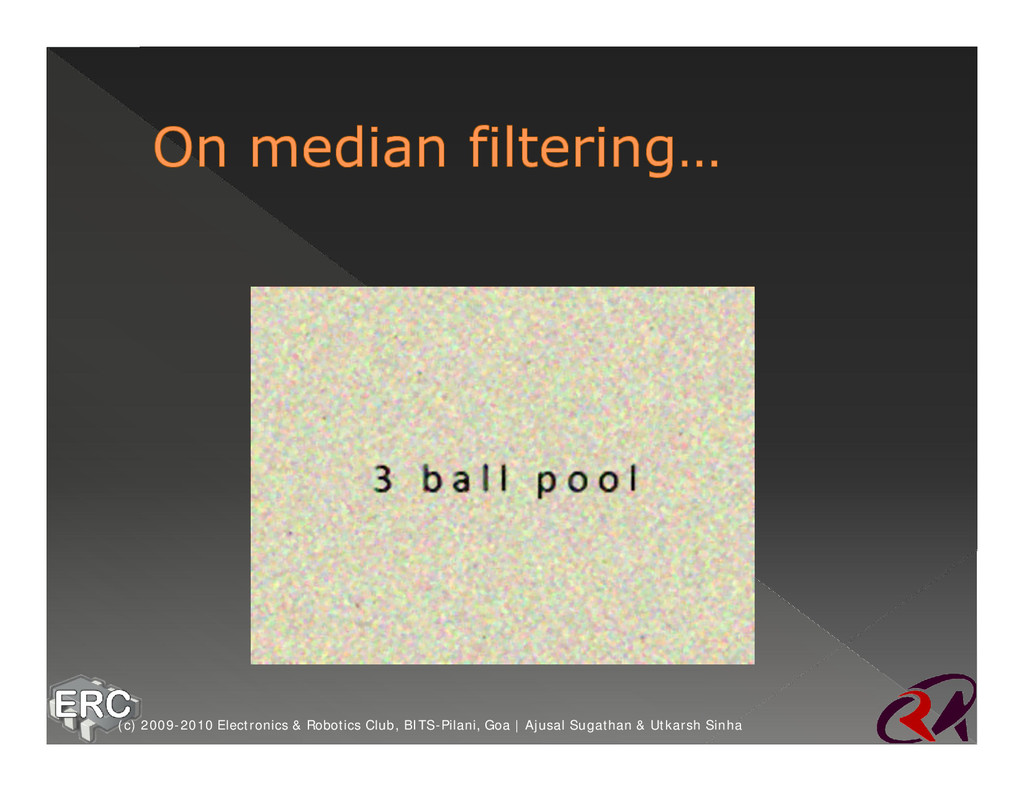
its neighbors, i.e. the value such that 50% of the values in the neighborhood are above, and 50% are below ž This can be difficult and costly to implement due to the need for sorting of the values ž However, this method is generally very good at preserving edges (c) 2009-2010 Electronics & Robotics Club, BITS-Pilani, Goa | Ajusal Sugathan & Utkarsh Sinha
ž The median is calculated by first sorting all the pixel values from the surrounding neighborhood into numerical order and then replacing the pixel being considered with the middle pixel value ž If the neighborhood under consideration contains an even number of pixels, the average of the two middle pixel values is used (c) 2009-2010 Electronics & Robotics Club, BITS-Pilani, Goa | Ajusal Sugathan & Utkarsh Sinha
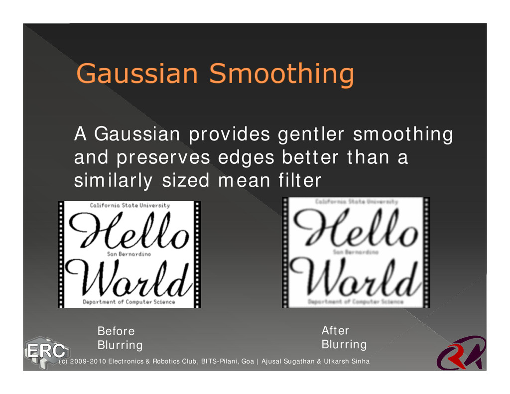
ž The effect of Gaussian smoothing is to blur an image ž The Gaussian outputs a `weighted average' of each pixel's neighborhood, with the average weighted more towards the value of the central pixels (c) 2009-2010 Electronics & Robotics Club, BITS-Pilani, Goa | Ajusal Sugathan & Utkarsh Sinha
than a similarly sized mean filter (c) 2009-2010 Electronics & Robotics Club, BITS-Pilani, Goa | Ajusal Sugathan & Utkarsh Sinha Before Blurring After Blurring
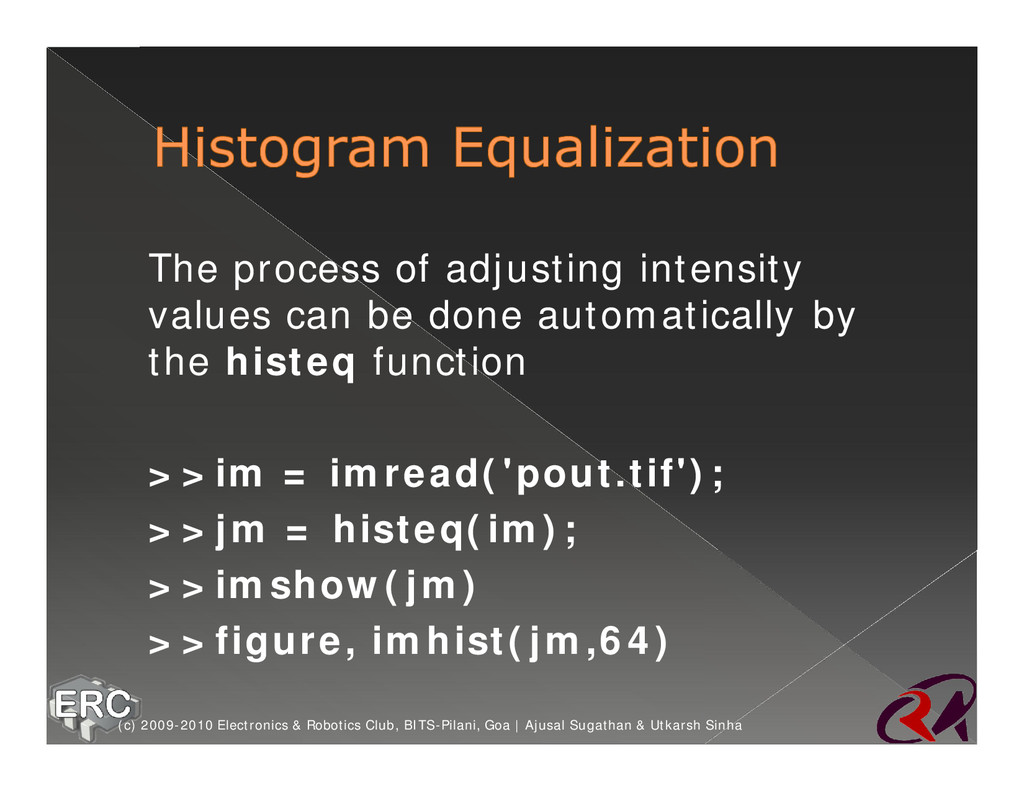
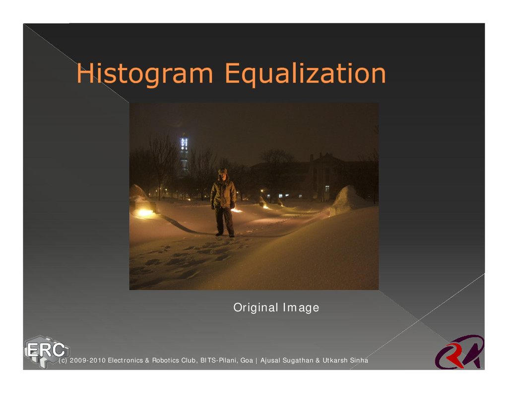
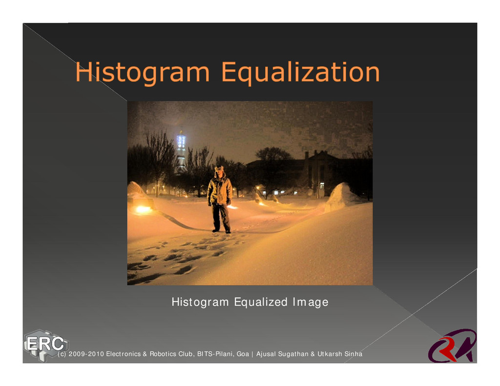
to eliminate noise due to changing lighting conditions etc ž Transforms the values in an intensity image so that the histogram of the output image approximately matches a specified histogram (c) 2009-2010 Electronics & Robotics Club, BITS-Pilani, Goa | Ajusal Sugathan & Utkarsh Sinha
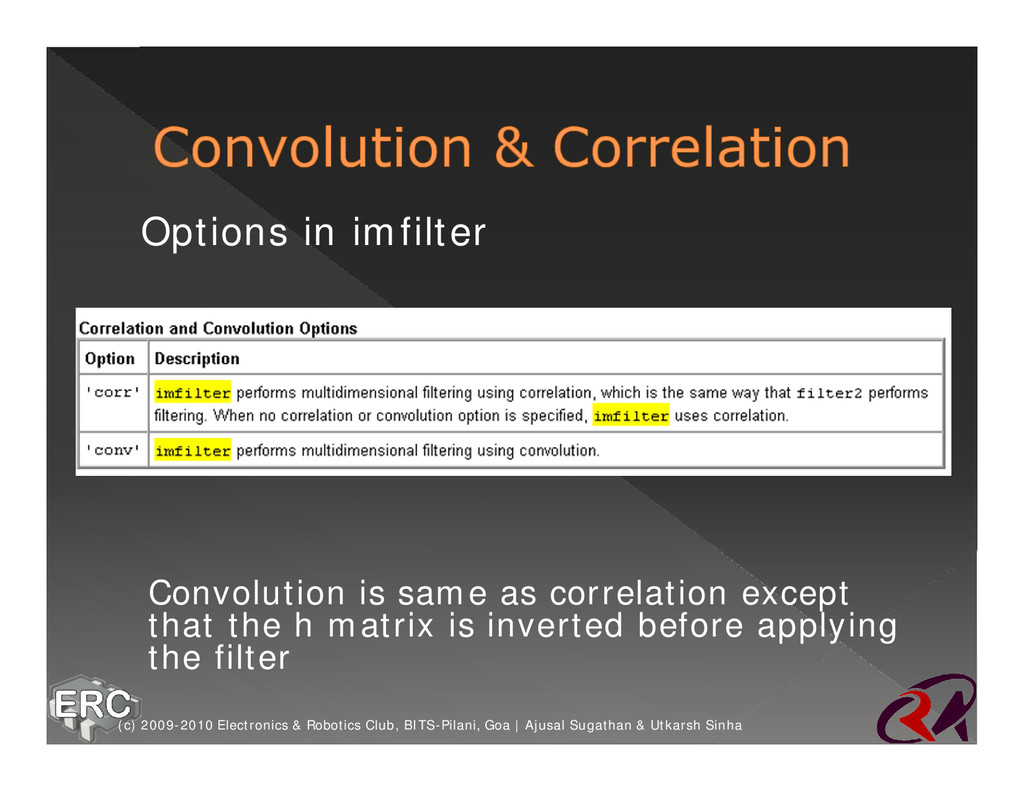
filters In MATLAB ž B = imfilter(A,H,’option’) filters the multidimensional array A with the multidimensional filter H ž The array A can be a nonsparse numeric array of any class and dimension ž The result B has the same size and class as A (c) 2009-2010 Electronics & Robotics Club, BITS-Pilani, Goa | Ajusal Sugathan & Utkarsh Sinha
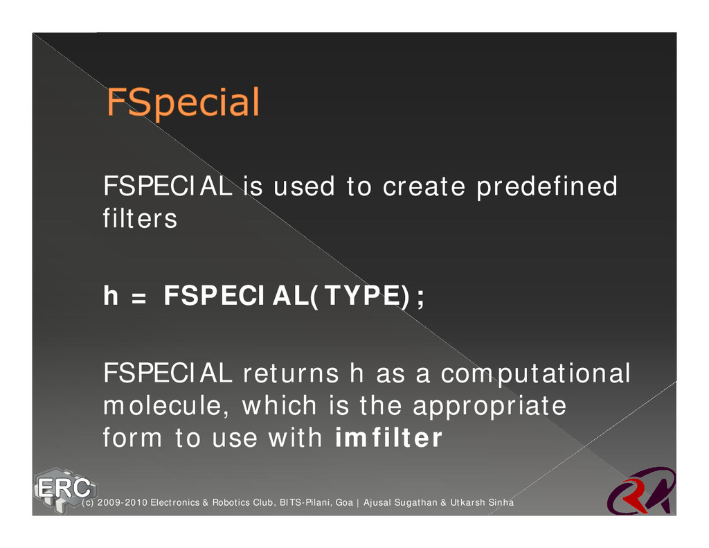
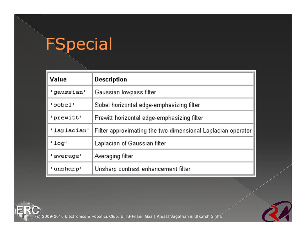
= FSPECIAL(TYPE); ž FSPECIAL returns h as a computational molecule, which is the appropriate form to use with imfilter (c) 2009-2010 Electronics & Robotics Club, BITS-Pilani, Goa | Ajusal Sugathan & Utkarsh Sinha
= FSPECIAL(TYPE); ž FSPECIAL returns h as a computational molecule, which is the appropriate form to use with imfilter (c) 2009-2010 Electronics & Robotics Club, BITS-Pilani, Goa | Ajusal Sugathan & Utkarsh Sinha
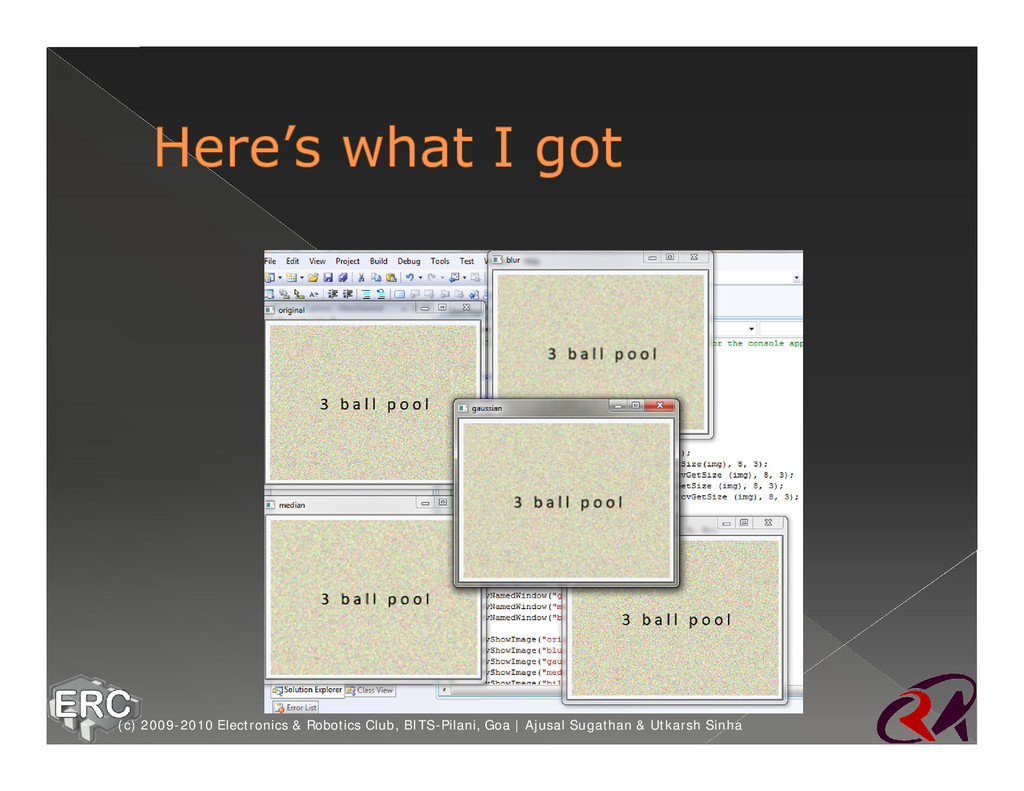
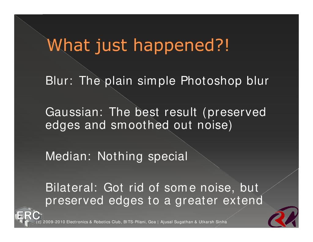
best result (preserved edges and smoothed out noise) ž Median: Nothing special ž Bilateral: Got rid of some noise, but preserved edges to a greater extend (c) 2009-2010 Electronics & Robotics Club, BITS-Pilani, Goa | Ajusal Sugathan & Utkarsh Sinha
we’ll code it ourselves ž And this will be a good exercise for getting better at OpenCV (c) 2009-2010 Electronics & Robotics Club, BITS-Pilani, Goa | Ajusal Sugathan & Utkarsh Sinha
imgGreen[25]; IplImage* imgBlue[25]; Holds the R, G and B channels separately for each of the 25 images (c) 2009-2010 Electronics & Robotics Club, BITS-Pilani, Goa | Ajusal Sugathan & Utkarsh Sinha
for green and 25 for blues ž Loaded 25 color images in the loop ž Split each image, and stored in an appropriate grayscale image (c) 2009-2010 Electronics & Robotics Club, BITS-Pilani, Goa | Ajusal Sugathan & Utkarsh Sinha
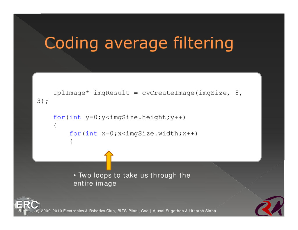
IplImage* imgResultGreen = cvCreateImage(imgSize, 8, 1); IplImage* imgResultBlue = cvCreateImage(imgSize, 8, 1); IplImage* imgResult = cvCreateImage(imgSize, 8, 3); • This will hold the final, filtered image • It will be a combination of the grayscale channels imgResultRed, imgResultGreen and imgResultBlue (c) 2009-2010 Electronics & Robotics Club, BITS-Pilani, Goa | Ajusal Sugathan & Utkarsh Sinha
x=0;x<imgSize.width;x++) { • Two loops to take us through the entire image (c) 2009-2010 Electronics & Robotics Club, BITS-Pilani, Goa | Ajusal Sugathan & Utkarsh Sinha
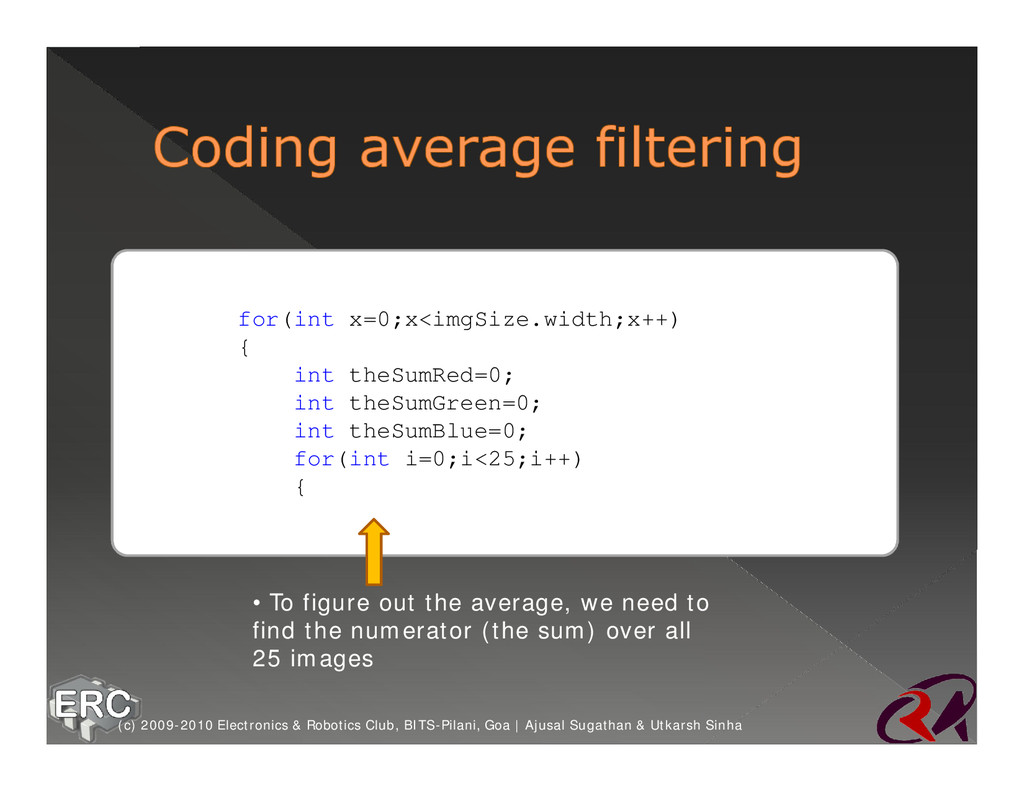
i=0;i<25;i++) { • To figure out the average, we need to find the numerator (the sum) over all 25 images (c) 2009-2010 Electronics & Robotics Club, BITS-Pilani, Goa | Ajusal Sugathan & Utkarsh Sinha
y, x); } • To figure out the average, we need to find the numerator (the sum) over all 25 images (c) 2009-2010 Electronics & Robotics Club, BITS-Pilani, Goa | Ajusal Sugathan & Utkarsh Sinha
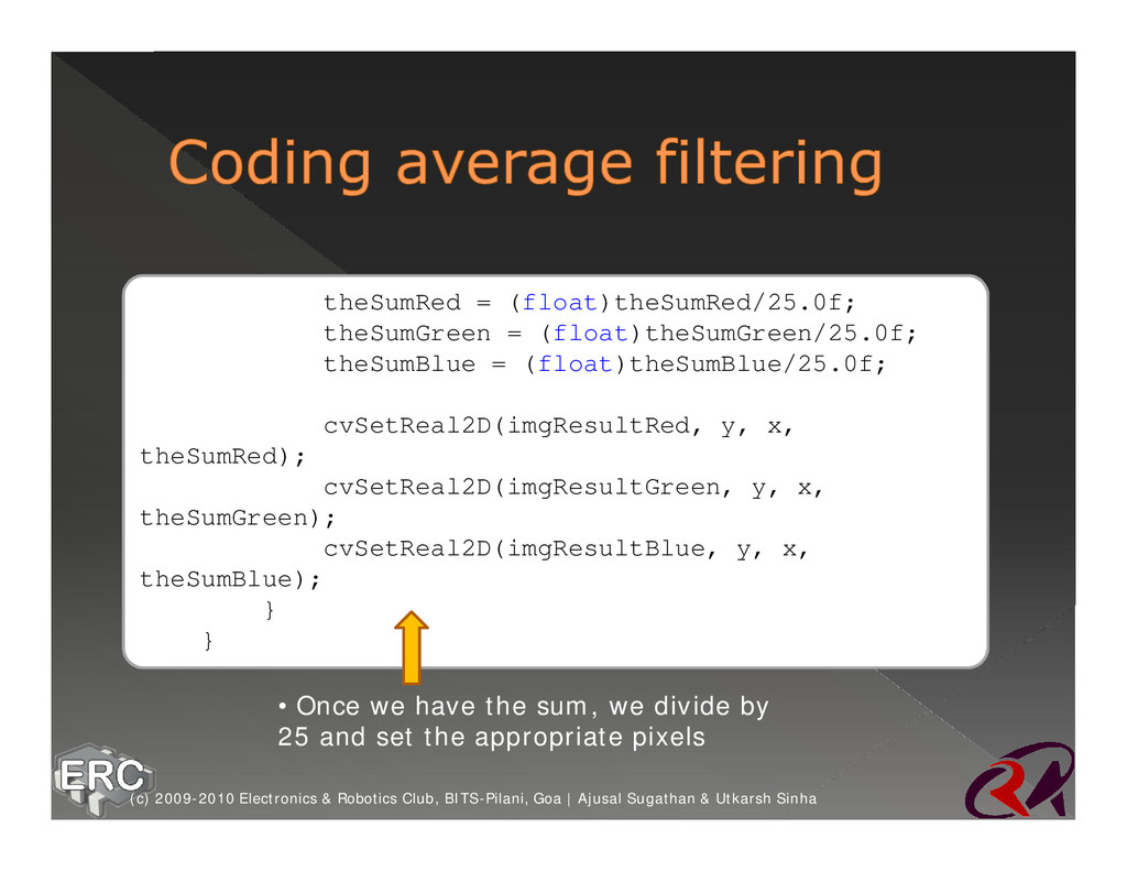
y, x, theSumRed); cvSetReal2D(imgResultGreen, y, x, theSumGreen); cvSetReal2D(imgResultBlue, y, x, theSumBlue); } } • Once we have the sum, we divide by 25 and set the appropriate pixels (c) 2009-2010 Electronics & Robotics Club, BITS-Pilani, Goa | Ajusal Sugathan & Utkarsh Sinha
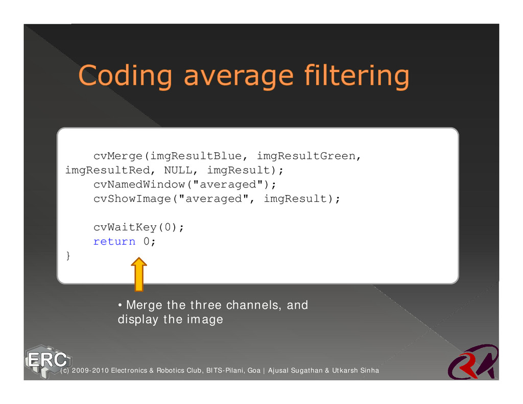
cvNamedWindow to create a window ž cvShowImage to show an image in a window (c) 2009-2010 Electronics & Robotics Club, BITS-Pilani, Goa | Ajusal Sugathan & Utkarsh Sinha
images ž cvSetReal2D to set the value at a pixel ž CvSize to store an image’s size (c) 2009-2010 Electronics & Robotics Club, BITS-Pilani, Goa | Ajusal Sugathan & Utkarsh Sinha
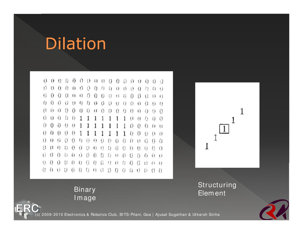
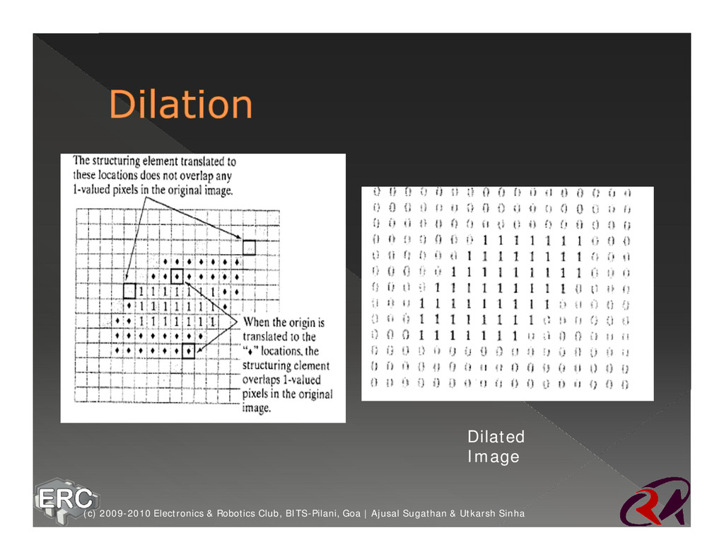
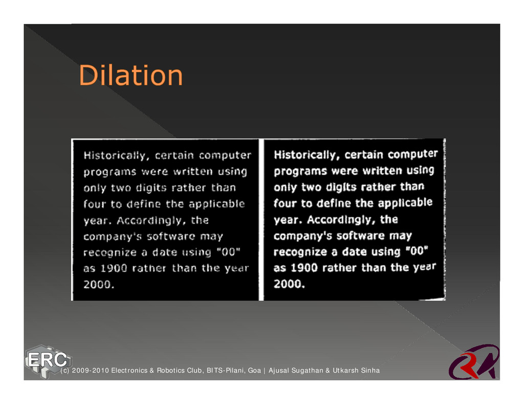
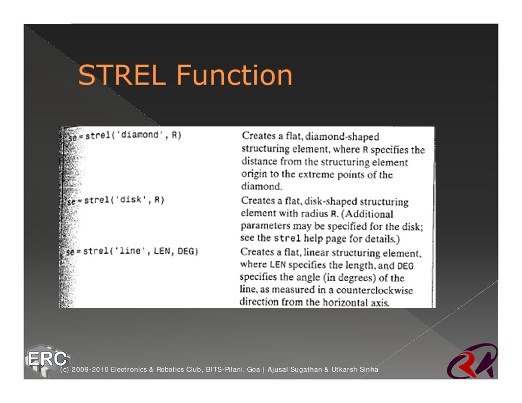
binary image ž The specific manner of thickening is controlled by a shape referred to as “structuring element” (c) 2009-2010 Electronics & Robotics Club, BITS-Pilani, Goa | Ajusal Sugathan & Utkarsh Sinha
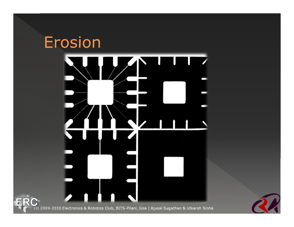
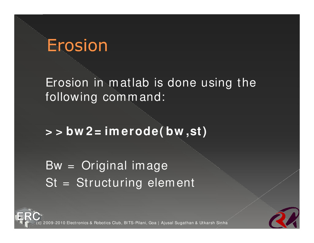
ž The manner of shrinkage is controlled by the structuring element (c) 2009-2010 Electronics & Robotics Club, BITS-Pilani, Goa | Ajusal Sugathan & Utkarsh Sinha
in various combinations ž An image can undergo a series for diltions and erosion using the same or different structuring element (c) 2009-2010 Electronics & Robotics Club, BITS-Pilani, Goa | Ajusal Sugathan & Utkarsh Sinha
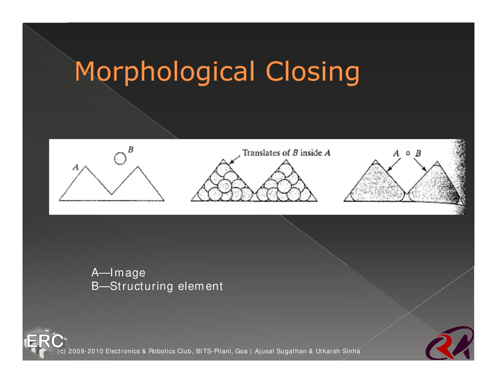
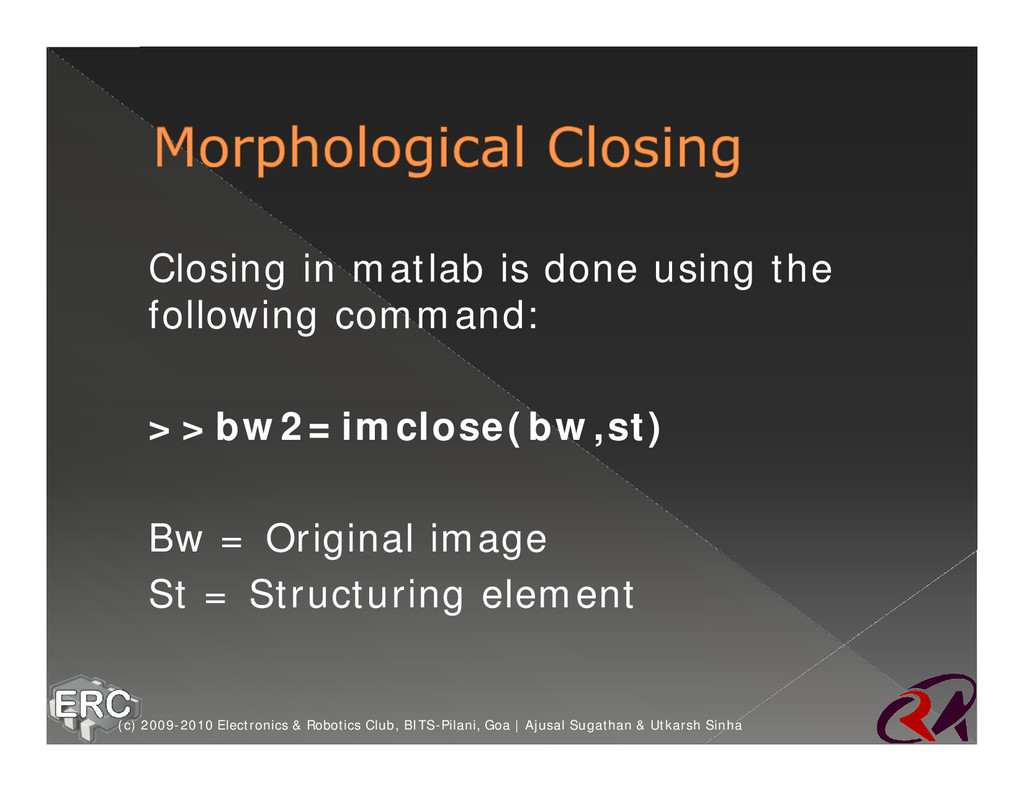
in various combinations ž An image can undergo a series for diltions and erosion using the same or different structuring element ž Two Common Kinds: › Morphological Opening › Morphological Closing (c) 2009-2010 Electronics & Robotics Club, BITS-Pilani, Goa | Ajusal Sugathan & Utkarsh Sinha
by the same structuring element ž They are used to smooth object contours, break thin connections and remove thin protrusions (c) 2009-2010 Electronics & Robotics Club, BITS-Pilani, Goa | Ajusal Sugathan & Utkarsh Sinha
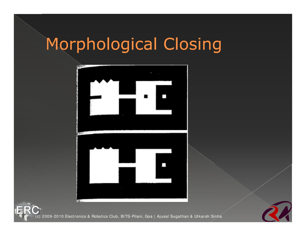
by the same structuring element ž They are used to smooth object contours like opening ž But unlike opening they generally join narrow breaks, fill long thin gulfs and fills holes smaller than the structuring element (c) 2009-2010 Electronics & Robotics Club, BITS-Pilani, Goa | Ajusal Sugathan & Utkarsh Sinha
are zeros) ž You can explicitly specify your structuring element as well ž Check the OpenCV Documentation for more information (c) 2009-2010 Electronics & Robotics Club, BITS-Pilani, Goa | Ajusal Sugathan & Utkarsh Sinha
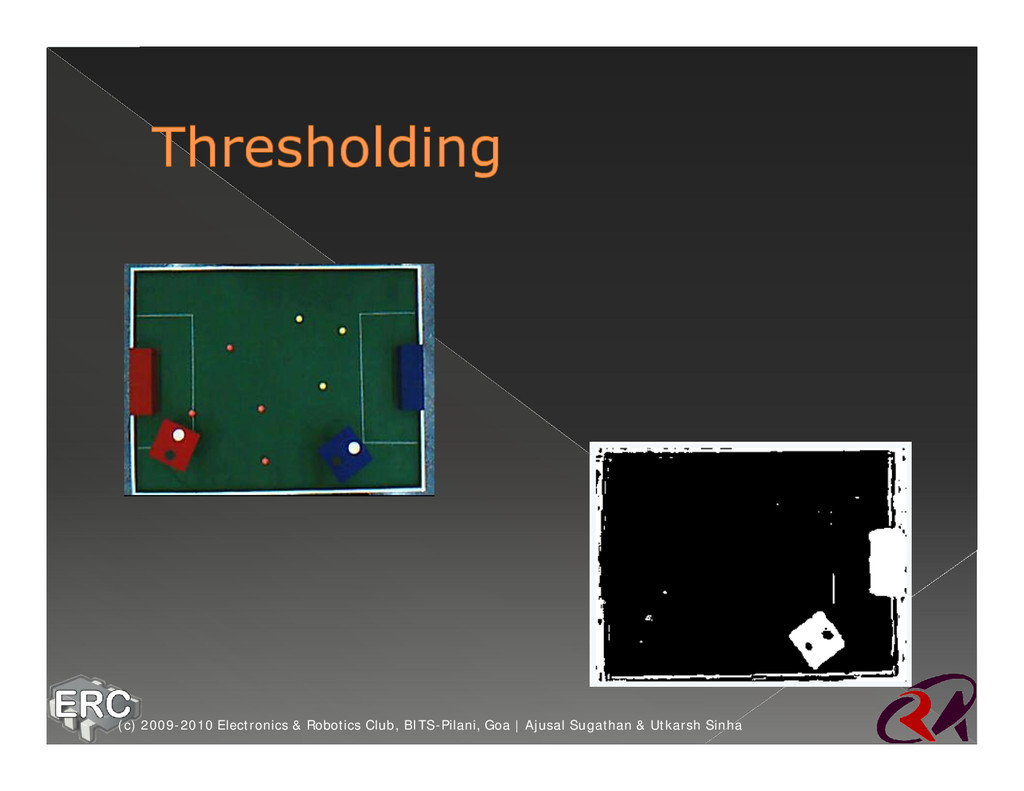
an image with millions of colors is tough ž Solution: Figure out interesting regions, and process them (c) 2009-2010 Electronics & Robotics Club, BITS-Pilani, Goa | Ajusal Sugathan & Utkarsh Sinha
it lies within a range, it is marked as “interesting” (or made white) ž Otherwise, it’s made black ž Figuring out the range depends on lighting, color, texture, etc (c) 2009-2010 Electronics & Robotics Club, BITS-Pilani, Goa | Ajusal Sugathan & Utkarsh Sinha
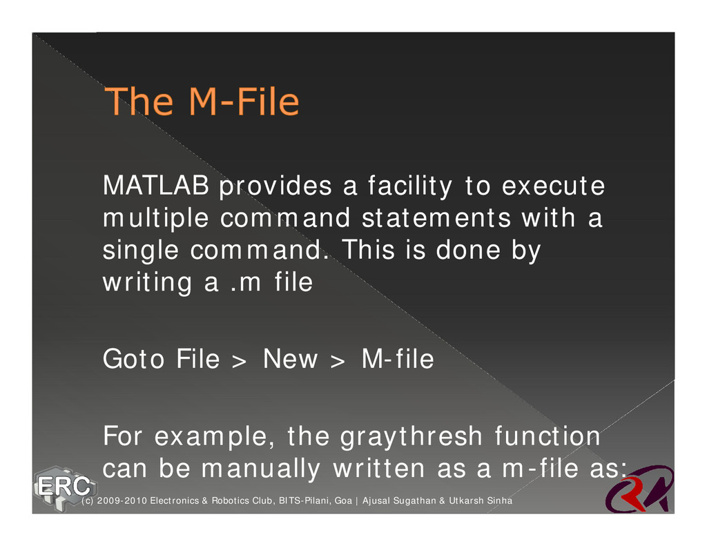
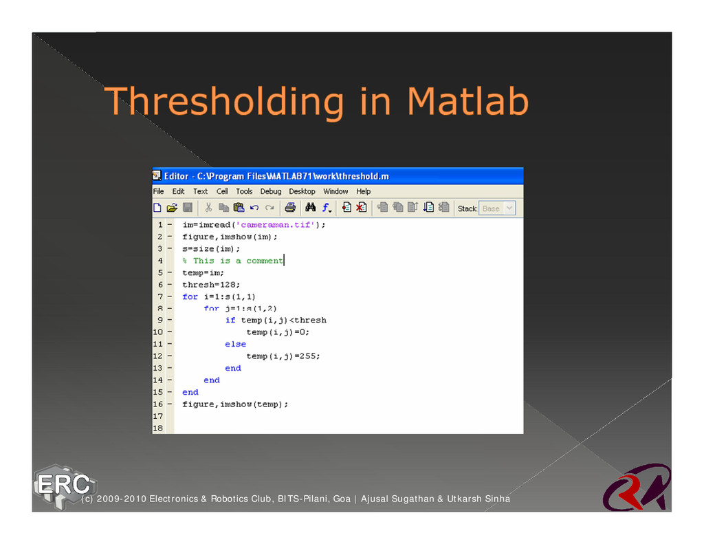
with a single command. This is done by writing a .m file ž Goto File > New > M-file ž For example, the graythresh function can be manually written as a m-file as: (c) 2009-2010 Electronics & Robotics Club, BITS-Pilani, Goa | Ajusal Sugathan & Utkarsh Sinha
the symbol ‘%’. A commented statement is not considered for execution ž M-files become a very handy utility for writing lengthy programs and can be saved and edited, as and when required ž We shall now see, how to define your own functions in MATLAB. (c) 2009-2010 Electronics & Robotics Club, BITS-Pilani, Goa | Ajusal Sugathan & Utkarsh Sinha
of logic ž Instead of rewriting the instruction set every time, you can define a function ž Syntax: ž Create an m-file and the top most statement of the file should be the function header ž function [return values] = function- name(arguments) (c) 2009-2010 Electronics & Robotics Club, BITS-Pilani, Goa | Ajusal Sugathan & Utkarsh Sinha
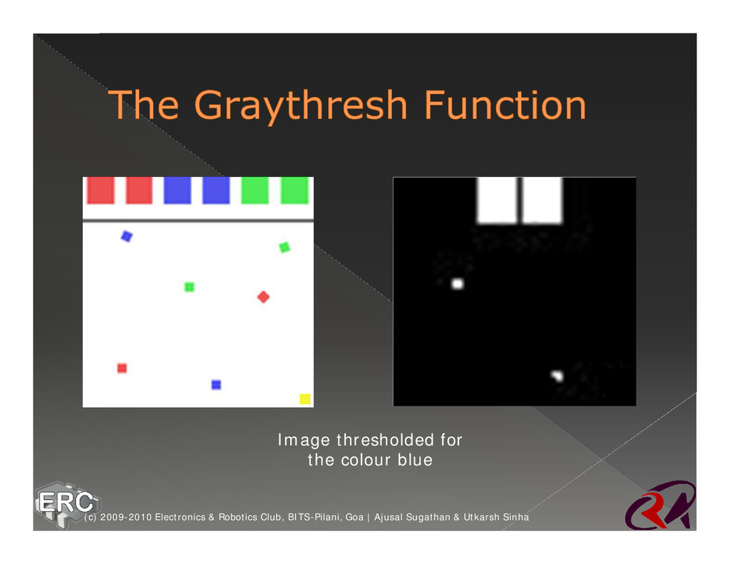
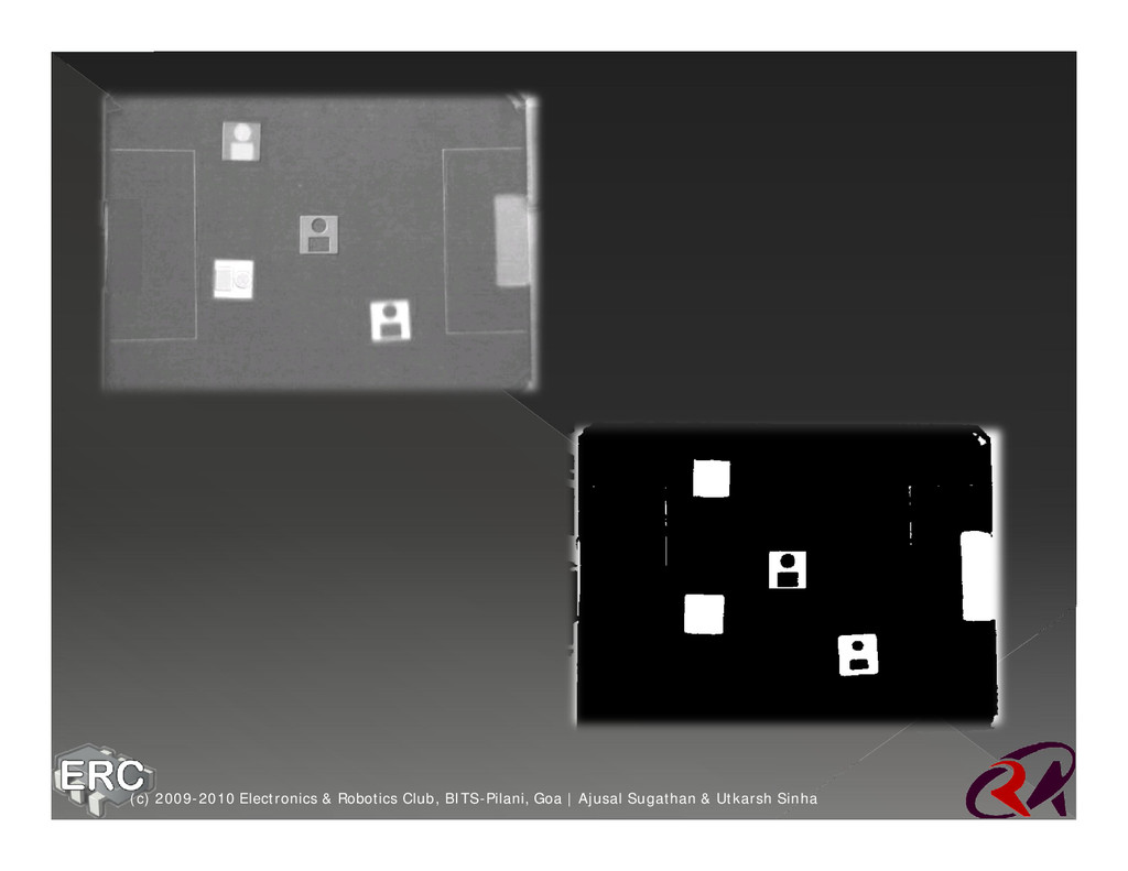
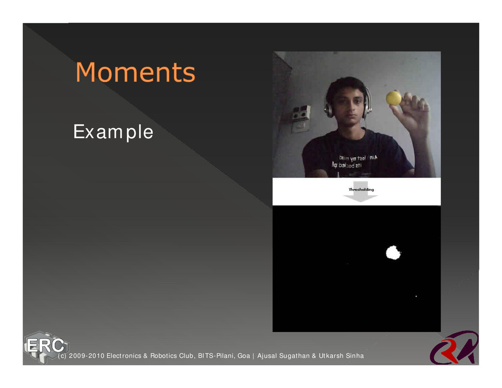
thresholding of grayscale images ž It uses the Otsu’s Method Of thresholding ž A sample thresholding opreation has been shown in the next slide (c) 2009-2010 Electronics & Robotics Club, BITS-Pilani, Goa | Ajusal Sugathan & Utkarsh Sinha
what exactly the threshold value should be ž Graythresh returns a value that lies in the range 0-1 ž This gives the level of threshold which is obtained by a complex method called the Otsu’s Method of Thresholding (c) 2009-2010 Electronics & Robotics Club, BITS-Pilani, Goa | Ajusal Sugathan & Utkarsh Sinha
multiplying by 255 ž Lets say, level=.4 ž Then threshold value for the grayscale image is: ž 0.4 x 255 =102 (c) 2009-2010 Electronics & Robotics Club, BITS-Pilani, Goa | Ajusal Sugathan & Utkarsh Sinha
the values below 102 have to be converted to 0 and values from 103-255 to the value 1 ž Conversion from grayscale to binary image is done using the function: ž >>imBW = im2bw(imGRAY,level); (c) 2009-2010 Electronics & Robotics Club, BITS-Pilani, Goa | Ajusal Sugathan & Utkarsh Sinha
function ž This function converts pixel intensities between 0 to level to zero intensity (black) and between level+1 to 255 to maximum (white) (c) 2009-2010 Electronics & Robotics Club, BITS-Pilani, Goa | Ajusal Sugathan & Utkarsh Sinha
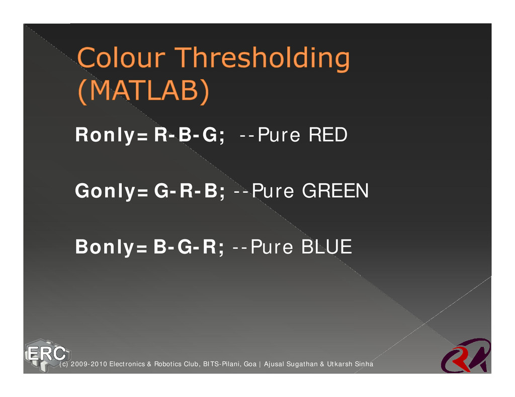
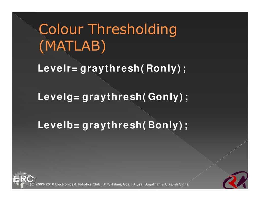
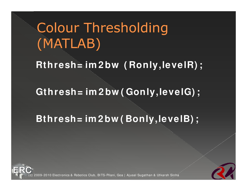
the graythresh function, the following have to be done: › Conversion of the RGB image into its 3 grayscale components › Subtracting each of these components from the other 2 to get the pure colour intensities › Finding level for each of the grayscale using graythresh › Thresholding the image using imbw and the level (c) 2009-2010 Electronics & Robotics Club, BITS-Pilani, Goa | Ajusal Sugathan & Utkarsh Sinha
Hue channel and thresholding it for different values ž Since the hue value of a single colour is constant it is relatively simple to threshold and gives better accuracy (c) 2009-2010 Electronics & Robotics Club, BITS-Pilani, Goa | Ajusal Sugathan & Utkarsh Sinha
Hue channel and thresholding it for different values ž Since the hue value of a single colour is constant it is relatively simple to threshold and gives better accuracy (c) 2009-2010 Electronics & Robotics Club, BITS-Pilani, Goa | Ajusal Sugathan & Utkarsh Sinha
the upper and lower bounds of the threshold levels ž These levels can be obtained by having a look at the range of hue values for the particular colour (c) 2009-2010 Electronics & Robotics Club, BITS-Pilani, Goa | Ajusal Sugathan & Utkarsh Sinha
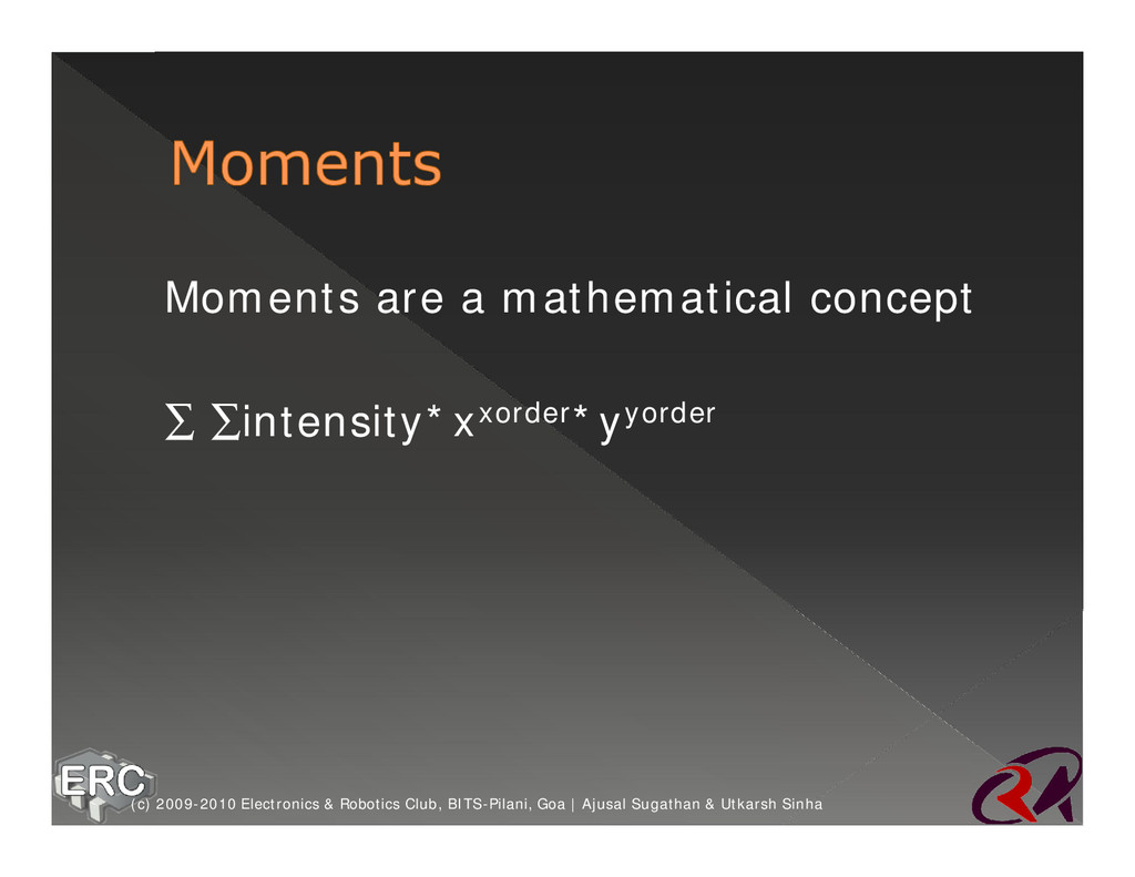
want useable information like centers, outlines, etc ž There geometrical properties can be found using many methods. We’ll talk about moments and contours only. (c) 2009-2010 Electronics & Robotics Club, BITS-Pilani, Goa | Ajusal Sugathan & Utkarsh Sinha
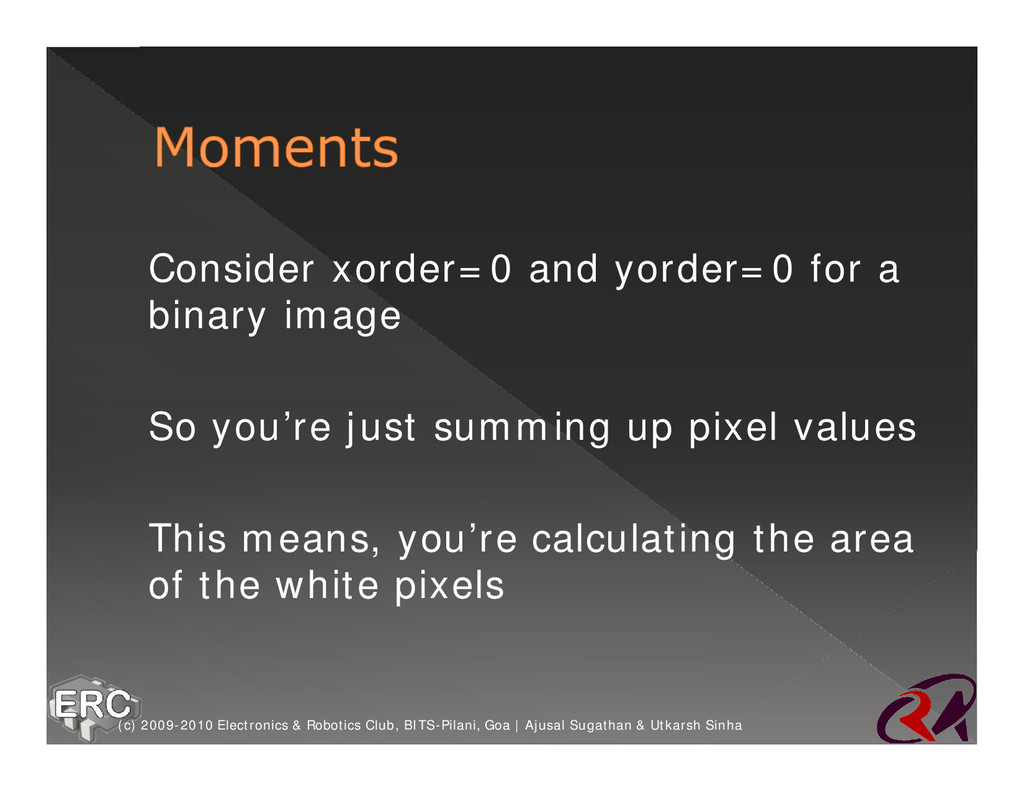
So you’re just summing up pixel values ž This means, you’re calculating the area of the white pixels (c) 2009-2010 Electronics & Robotics Club, BITS-Pilani, Goa | Ajusal Sugathan & Utkarsh Sinha
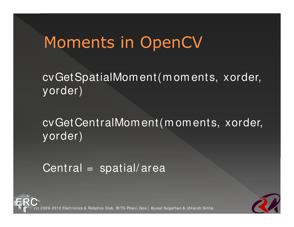
ž You sum only those x which are white ž So you’re calculating the numerator of an average (c) 2009-2010 Electronics & Robotics Club, BITS-Pilani, Goa | Ajusal Sugathan & Utkarsh Sinha
is the area of the image ž So, dividing this particular moment (xorder=1, yorder=0) by the earlier example (xorder=0, yorder=0) gives the average x ž This is the x coordinate of the centroid of the blob (c) 2009-2010 Electronics & Robotics Club, BITS-Pilani, Goa | Ajusal Sugathan & Utkarsh Sinha
the area is a zero order moment ž The centroid coordinate = a first order moment / the zero order moment (c) 2009-2010 Electronics & Robotics Club, BITS-Pilani, Goa | Ajusal Sugathan & Utkarsh Sinha
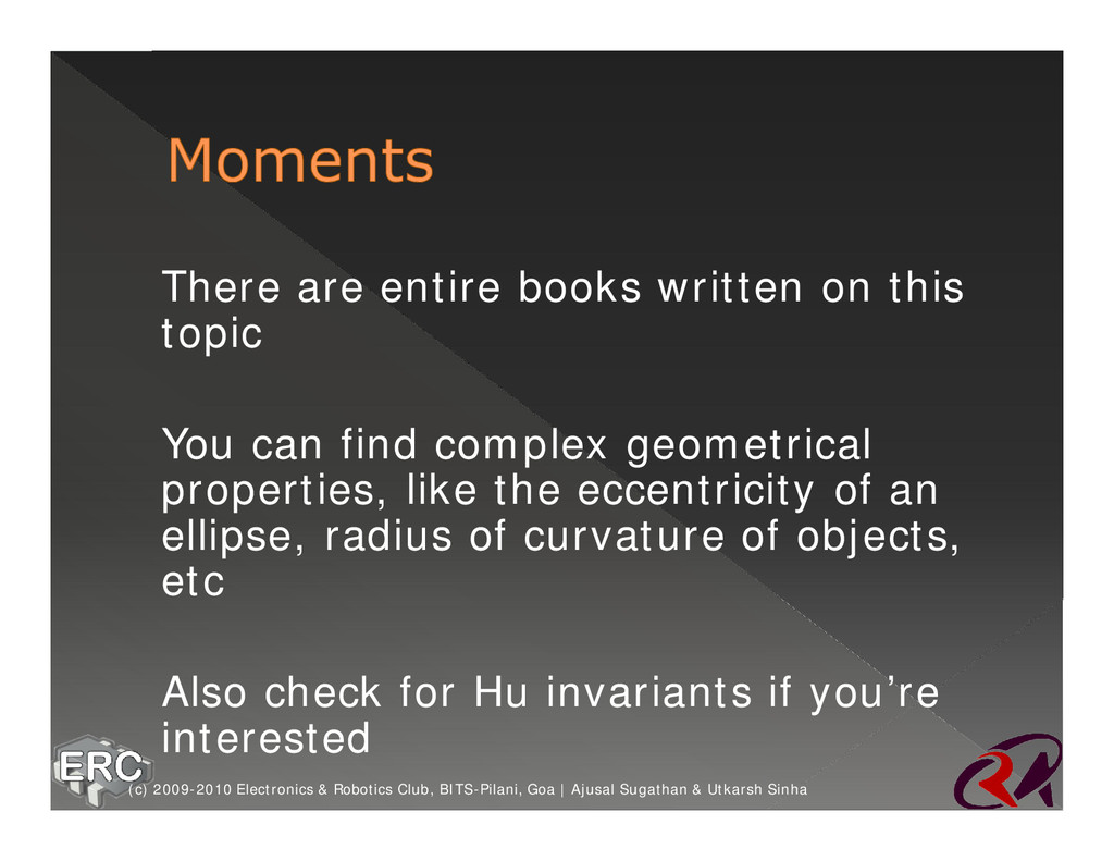
You can find complex geometrical properties, like the eccentricity of an ellipse, radius of curvature of objects, etc ž Also check for Hu invariants if you’re interested (c) 2009-2010 Electronics & Robotics Club, BITS-Pilani, Goa | Ajusal Sugathan & Utkarsh Sinha
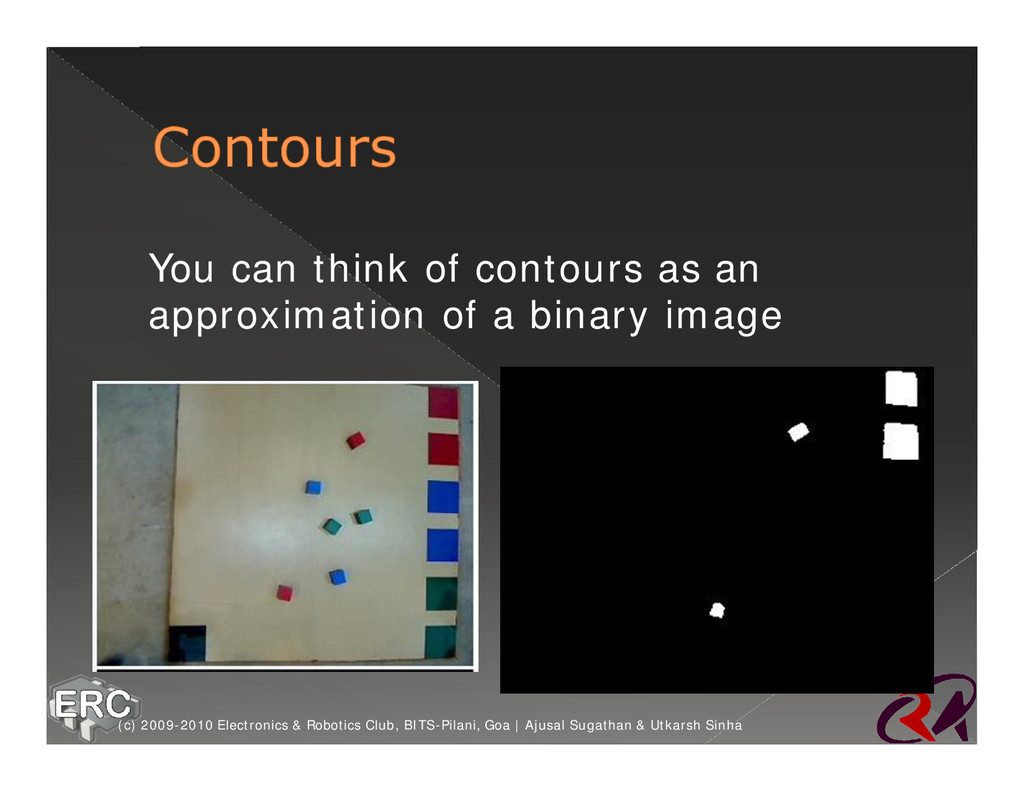
to each other forming separate blobs in an image ž They can be seperated out and labelled (c) 2009-2010 Electronics & Robotics Club, BITS-Pilani, Goa | Ajusal Sugathan & Utkarsh Sinha
the same size as BW, containing labels for the connected objects in BW ž n can have a value of either 4 or 8, where 4 specifies 4-connected objects and 8 specifies 8-connected objects; if the argument is omitted, it defaults to 8 (c) 2009-2010 Electronics & Robotics Club, BITS-Pilani, Goa | Ajusal Sugathan & Utkarsh Sinha
the same size as BW, containing labels for the connected objects in BW ž n can have a value of either 4 or 8, where 4 specifies 4-connected objects and 8 specifies 8-connected objects; if the argument is omitted, it defaults to 8 (c) 2009-2010 Electronics & Robotics Club, BITS-Pilani, Goa | Ajusal Sugathan & Utkarsh Sinha
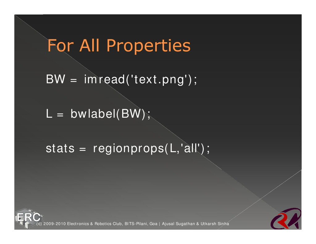
for each labeled region in the label matrix L ž The set of elements of L equal to 1 corresponds to region 1; the set of elements of L equal to 2 corresponds to region 2; and so on (c) 2009-2010 Electronics & Robotics Club, BITS-Pilani, Goa | Ajusal Sugathan & Utkarsh Sinha
ž 'Centroid'-- The center of mass of the region. Note that the first element of Centroid is the horizontal coordinate (or x-coordinate) of the center of mass, and the second element is the vertical coordinate (or y-coordinate) ž 'Orientation' -- Scalar; the angle (in degrees) between the x-axis and the major axis of the ellipse that has the same second-moments as the region. This property is supported only for 2-D input label matrices (c) 2009-2010 Electronics & Robotics Club, BITS-Pilani, Goa | Ajusal Sugathan & Utkarsh Sinha
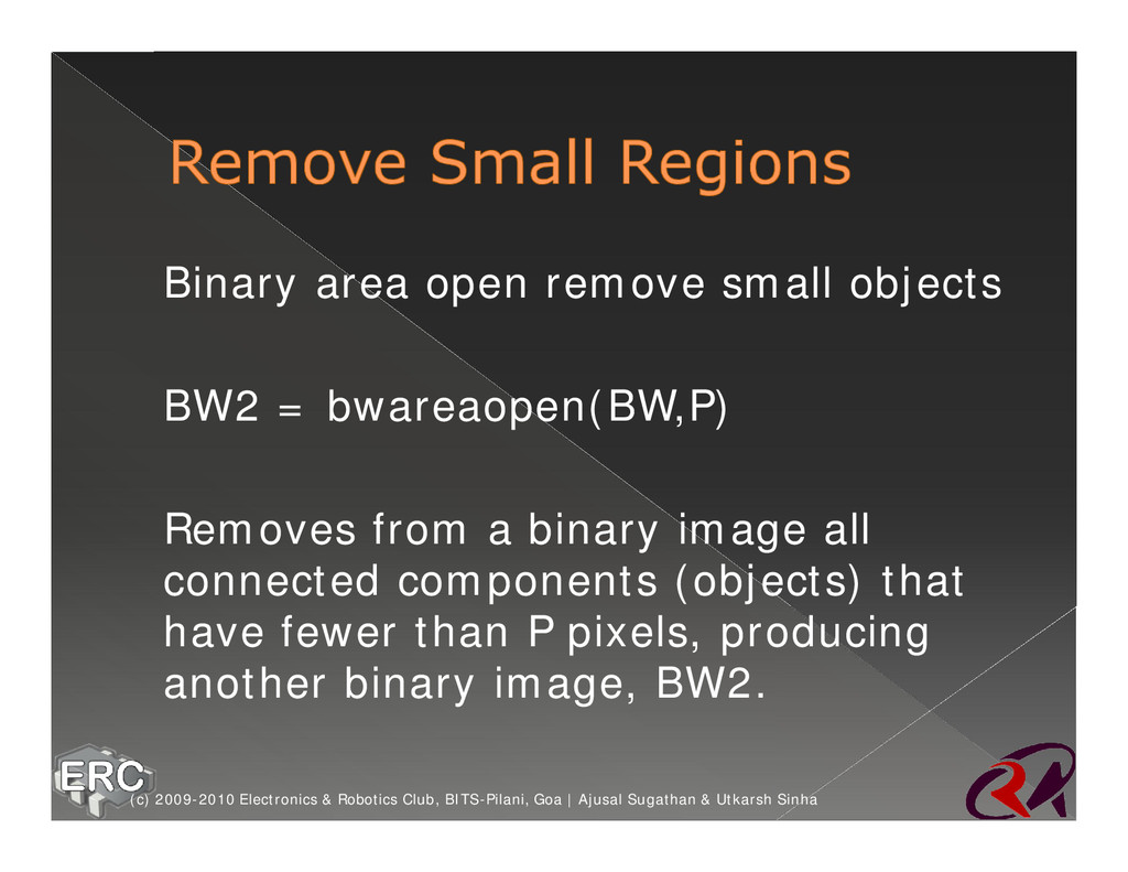
bwareaopen(BW,P) ž Removes from a binary image all connected components (objects) that have fewer than P pixels, producing another binary image, BW2. (c) 2009-2010 Electronics & Robotics Club, BITS-Pilani, Goa | Ajusal Sugathan & Utkarsh Sinha
single object ž If we have multiple objects in the same binary image (c) 2009-2010 Electronics & Robotics Club, BITS-Pilani, Goa | Ajusal Sugathan & Utkarsh Sinha
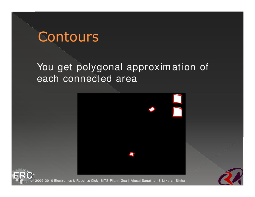
is: › Four “chains” of points › Each chain can have any number of points › In our case, each chain has four points (c) 2009-2010 Electronics & Robotics Club, BITS-Pilani, Goa | Ajusal Sugathan & Utkarsh Sinha
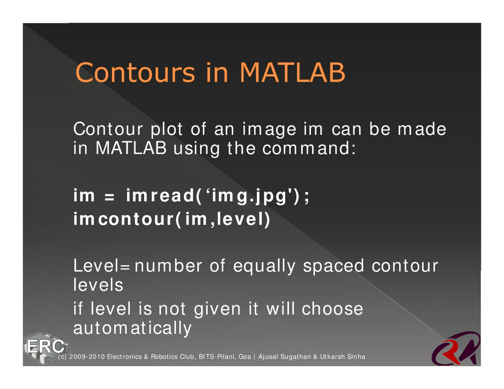
in MATLAB using the command: ž im = imread(‘img.jpg'); ž imcontour(im,level) ž Level=number of equally spaced contour levels ž if level is not given it will choose automatically (c) 2009-2010 Electronics & Robotics Club, BITS-Pilani, Goa | Ajusal Sugathan & Utkarsh Sinha
see some code to find out the squares in the thresholded image you saw (c) 2009-2010 Electronics & Robotics Club, BITS-Pilani, Goa | Ajusal Sugathan & Utkarsh Sinha
chains are stored in contours • result is a temporary variable • storage is for temporary memory allocation (c) 2009-2010 Electronics & Robotics Club, BITS-Pilani, Goa | Ajusal Sugathan & Utkarsh Sinha
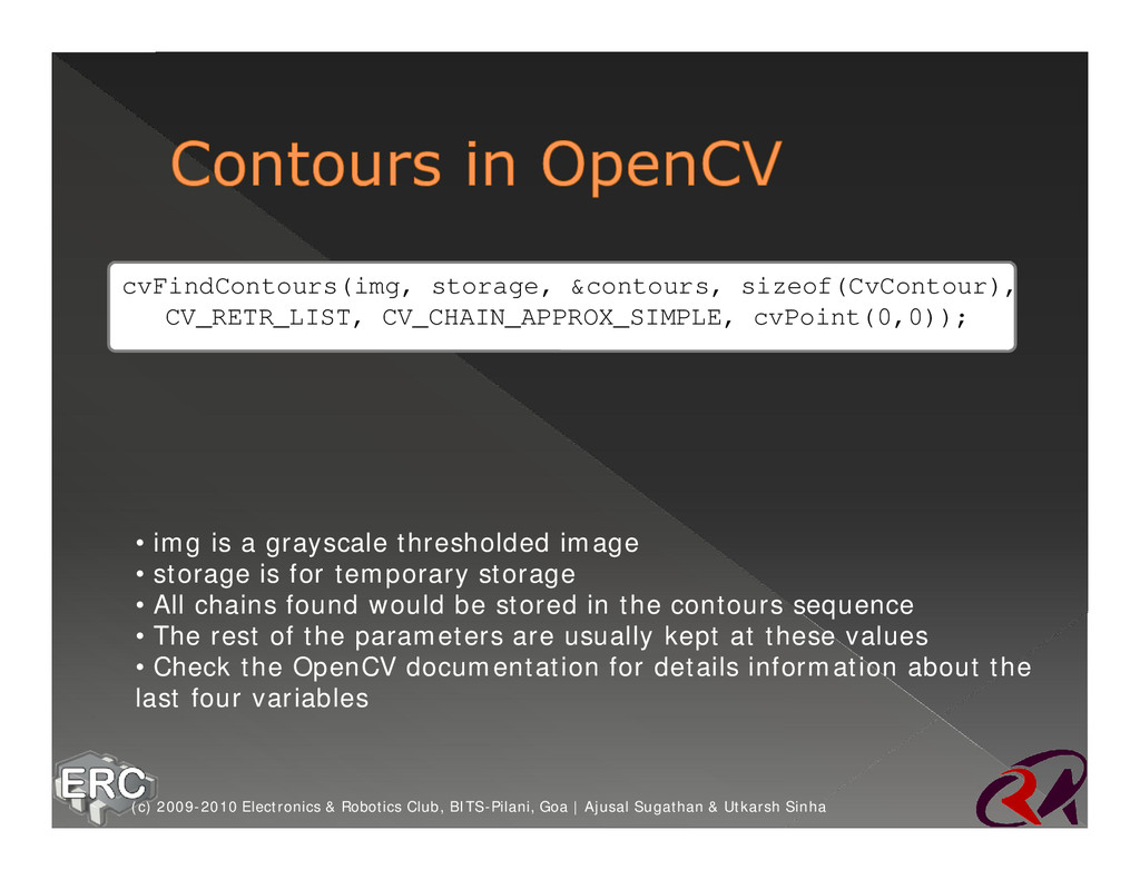
a grayscale thresholded image • storage is for temporary storage • All chains found would be stored in the contours sequence • The rest of the parameters are usually kept at these values • Check the OpenCV documentation for details information about the last four variables (c) 2009-2010 Electronics & Robotics Club, BITS-Pilani, Goa | Ajusal Sugathan & Utkarsh Sinha
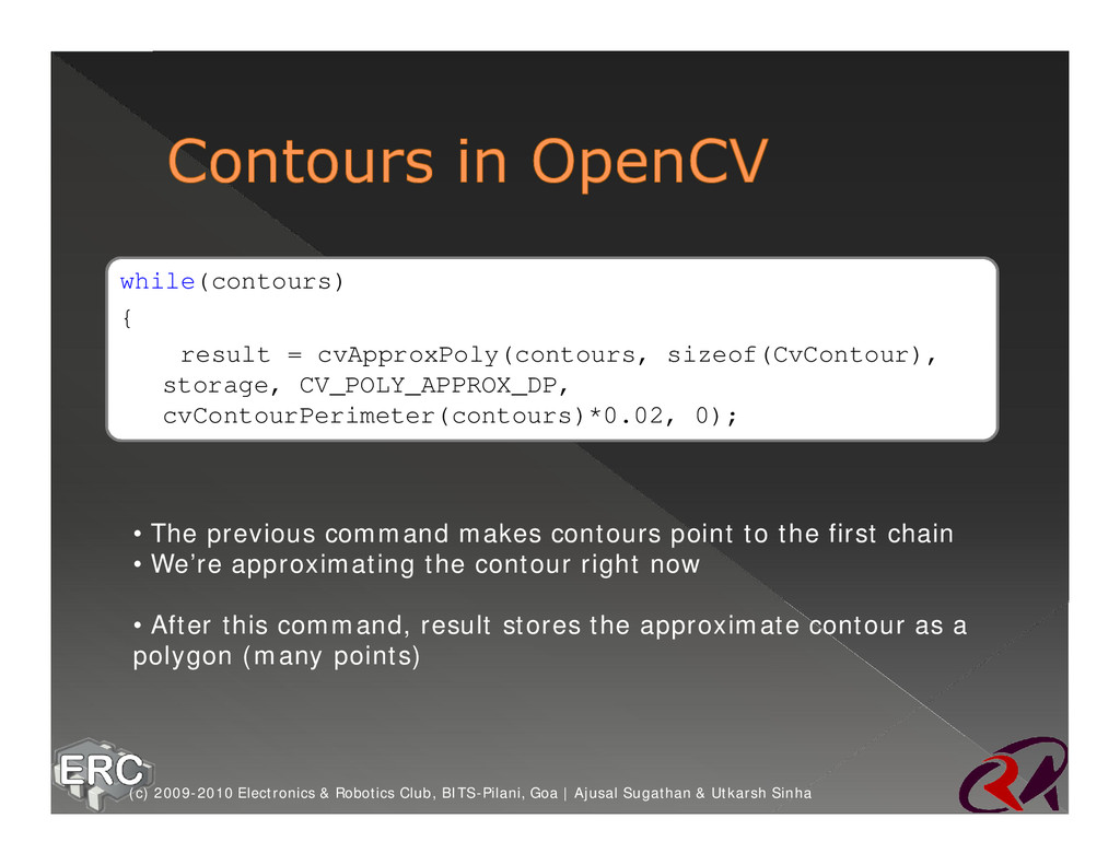
• The previous command makes contours point to the first chain • We’re approximating the contour right now • After this command, result stores the approximate contour as a polygon (many points) (c) 2009-2010 Electronics & Robotics Club, BITS-Pilani, Goa | Ajusal Sugathan & Utkarsh Sinha
} • We’re looking for quadrilaterals, so we check if the number of points in this particular polygon is 4 • Then, get extract each point using the command cvGetSeqElem • Once you have the points, you can actually check the shape of the object as well (by checking angles, lengths, etc) (c) 2009-2010 Electronics & Robotics Club, BITS-Pilani, Goa | Ajusal Sugathan & Utkarsh Sinha
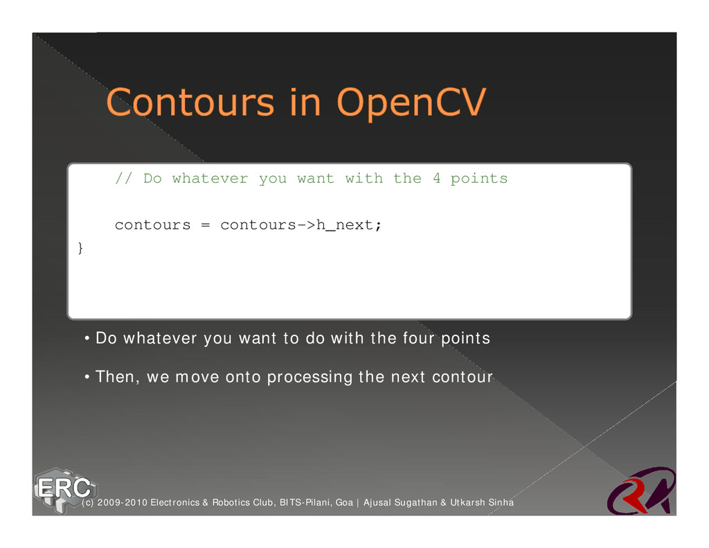
= contours->h_next; } • Do whatever you want to do with the four points • Then, we move onto processing the next contour (c) 2009-2010 Electronics & Robotics Club, BITS-Pilani, Goa | Ajusal Sugathan & Utkarsh Sinha
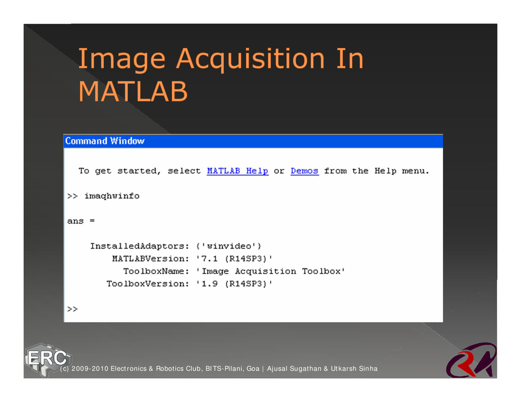
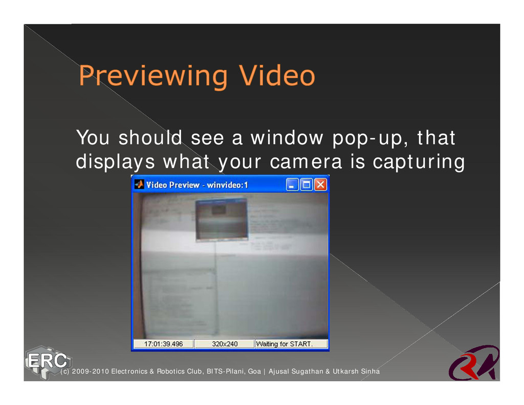
images ž Now-a-days most of the cameras are available with USB interface ž Once you install the driver for the camera, the computer detects the device whenever you connect it (c) 2009-2010 Electronics & Robotics Club, BITS-Pilani, Goa | Ajusal Sugathan & Utkarsh Sinha
available for your camera ž MATLAB has built-in adaptors for accessing these devices ž An adaptor is a software that MATLAB uses to communicate with an image acquisition device (c) 2009-2010 Electronics & Robotics Club, BITS-Pilani, Goa | Ajusal Sugathan & Utkarsh Sinha
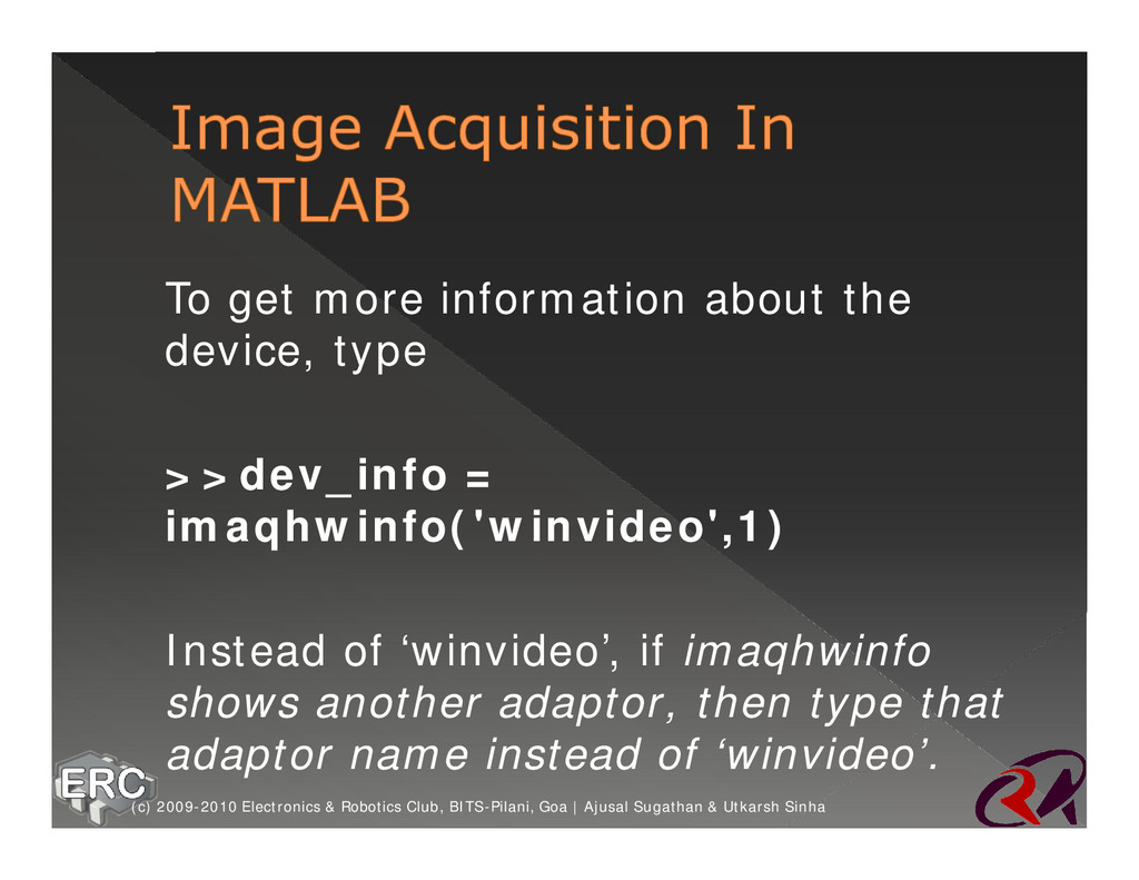
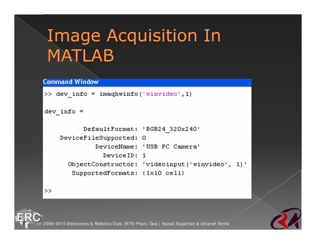
>>dev_info = imaqhwinfo('winvideo',1) ž Instead of ‘winvideo’, if imaqhwinfo shows another adaptor, then type that adaptor name instead of ‘winvideo’. (c) 2009-2010 Electronics & Robotics Club, BITS-Pilani, Goa | Ajusal Sugathan & Utkarsh Sinha
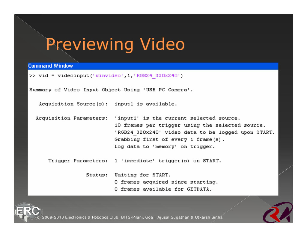
by defining an object and associate it with the device ž >>vid=videoinput(‘winvideo’,1,‘RGB24 _320x240’) (c) 2009-2010 Electronics & Robotics Club, BITS-Pilani, Goa | Ajusal Sugathan & Utkarsh Sinha
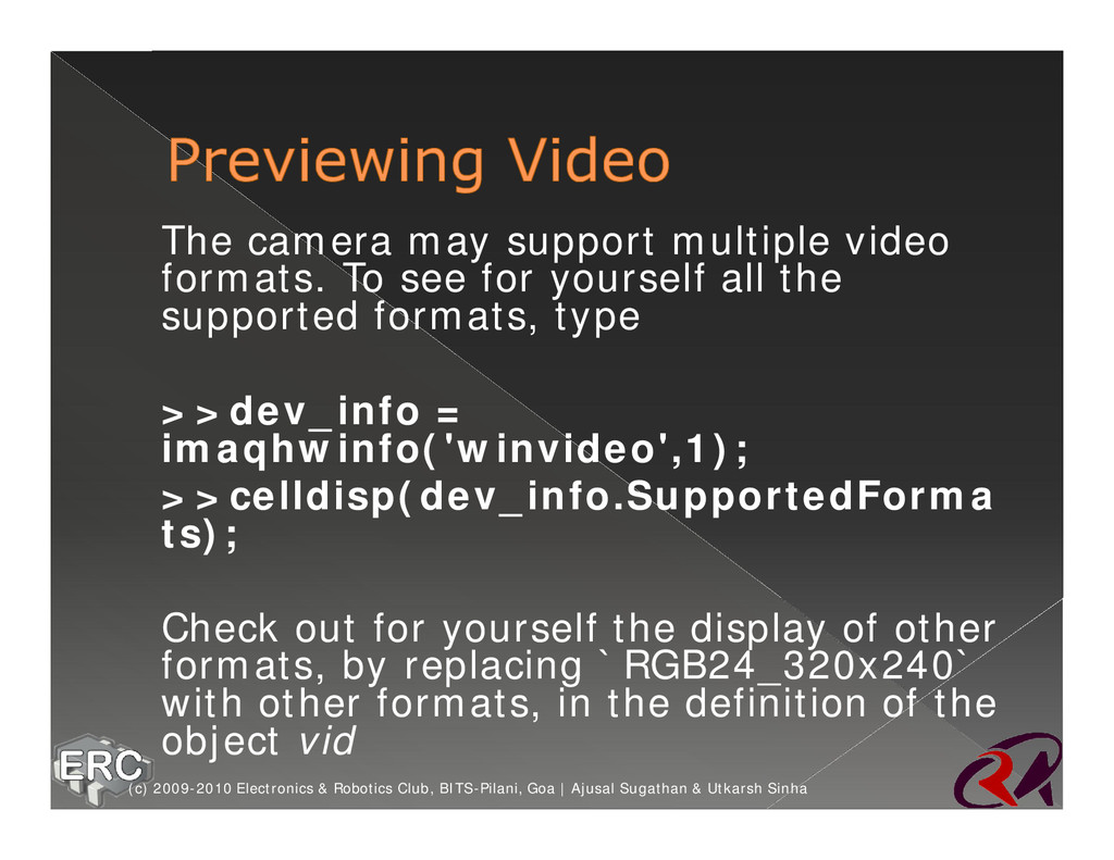
Sugathan & Utkarsh Sinha ž The camera may support multiple video formats. To see for yourself all the supported formats, type ž >>dev_info = imaqhwinfo('winvideo',1); ž >>celldisp(dev_info.SupportedForma ts); ž Check out for yourself the display of other formats, by replacing `RGB24_320x240` with other formats, in the definition of the object vid
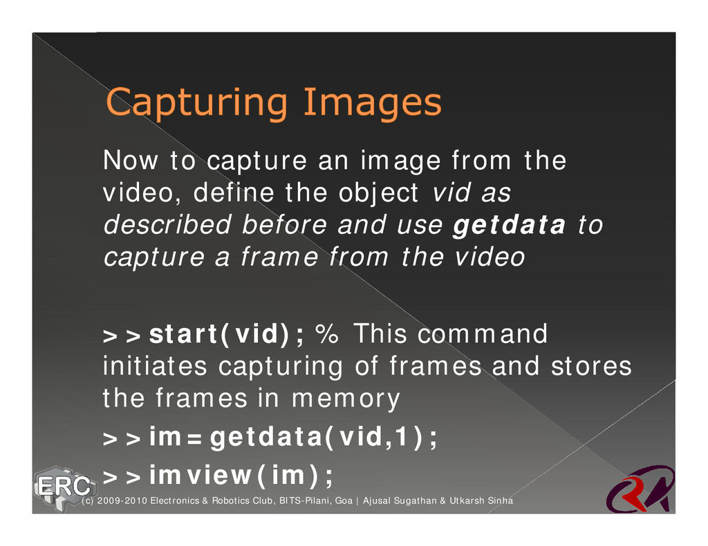
Sugathan & Utkarsh Sinha ž Now to capture an image from the video, define the object vid as described before and use getdata to capture a frame from the video ž >>start(vid); % This command initiates capturing of frames and stores the frames in memory ž >>im=getdata(vid,1); ž >>imview(im);
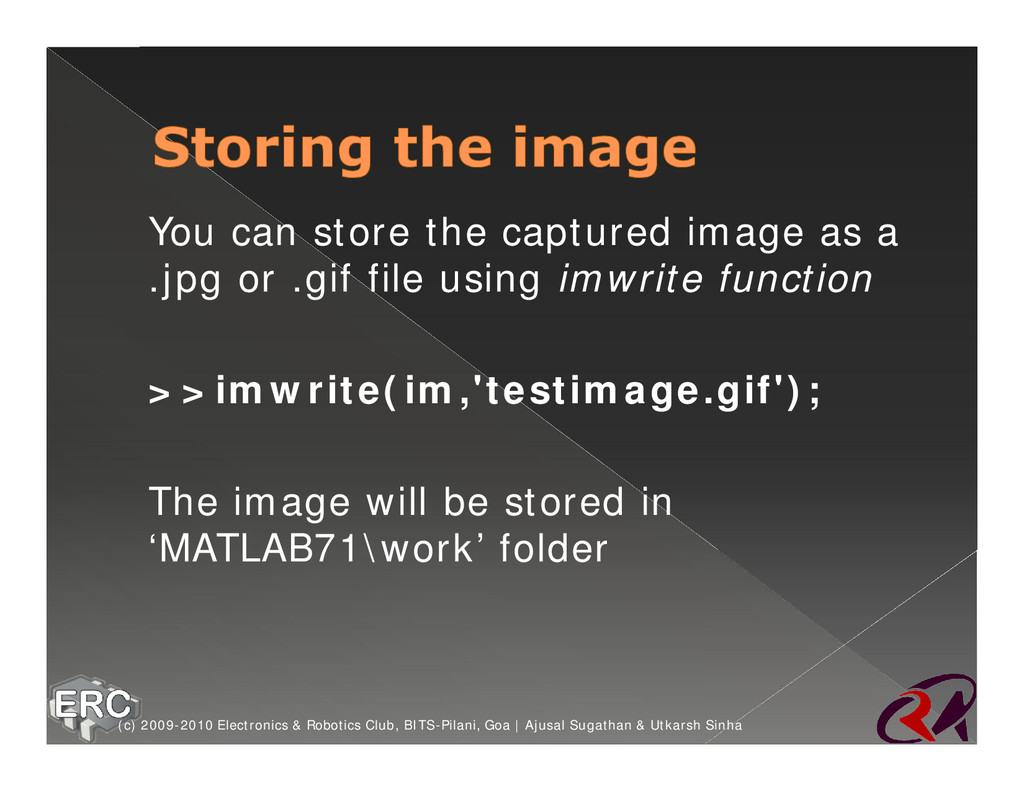
Sugathan & Utkarsh Sinha ž You can store the captured image as a .jpg or .gif file using imwrite function ž >>imwrite(im,'testimage.gif'); ž The image will be stored in ‘MATLAB71\work’ folder
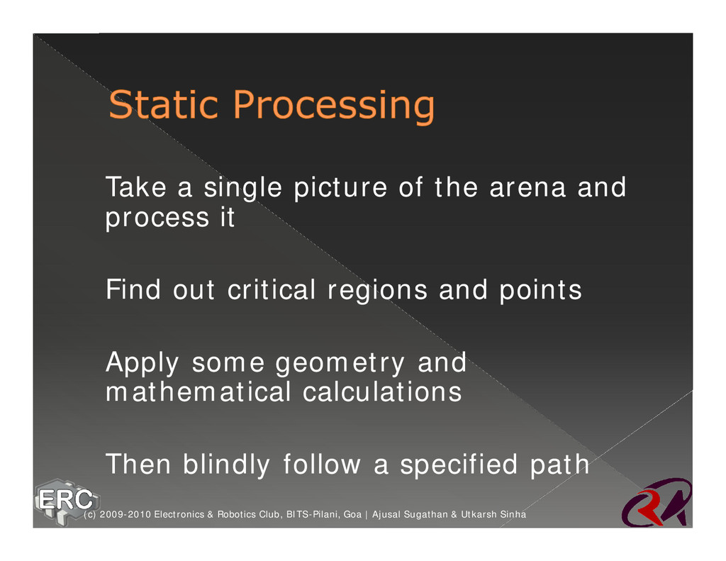
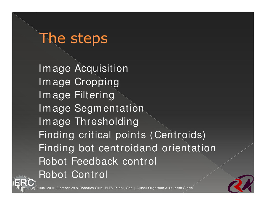
it ž Find out critical regions and points ž Apply some geometry and mathematical calculations ž Then blindly follow a specified path (c) 2009-2010 Electronics & Robotics Club, BITS-Pilani, Goa | Ajusal Sugathan & Utkarsh Sinha
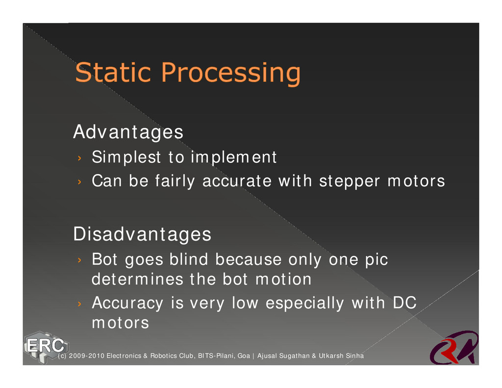
accurate with stepper motors ž Disadvantages › Bot goes blind because only one pic determines the bot motion › Accuracy is very low especially with DC motors (c) 2009-2010 Electronics & Robotics Club, BITS-Pilani, Goa | Ajusal Sugathan & Utkarsh Sinha
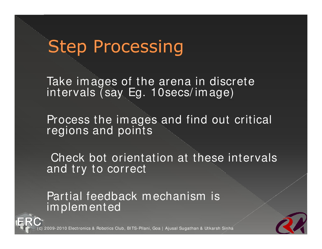
Eg. 10secs/image) ž Process the images and find out critical regions and points ž Check bot orientation at these intervals and try to correct ž Partial feedback mechanism is implemented (c) 2009-2010 Electronics & Robotics Club, BITS-Pilani, Goa | Ajusal Sugathan & Utkarsh Sinha
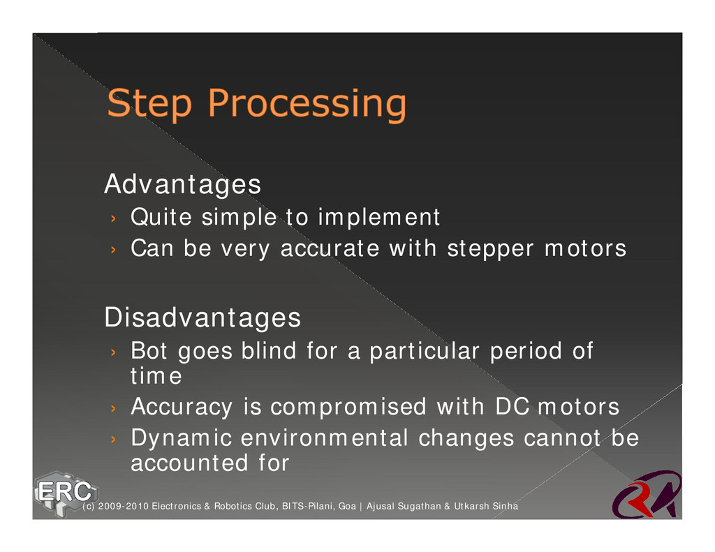
Sugathan & Utkarsh Sinha ž Advantages › Quite simple to implement › Can be very accurate with stepper motors ž Disadvantages › Bot goes blind for a particular period of time › Accuracy is compromised with DC motors › Dynamic environmental changes cannot be accounted for
frame rate ž Process the images and find out critical regions and points ž Check bot orientation at every frame and correct ž Complete feedback mechanism is implemented (c) 2009-2010 Electronics & Robotics Club, BITS-Pilani, Goa | Ajusal Sugathan & Utkarsh Sinha
Sugathan & Utkarsh Sinha ž Advantages › Very accurate for both DC and Stepper motors › Gives dynamic feedback and accounts for changing environment › Can give bot orientation at each point of time ž Disadvantages › Requires more processing power › Requires more memory for taking so many images
real application ž Dynamic feedback systems give excellent accuracy and precision and hence is the best approach (c) 2009-2010 Electronics & Robotics Club, BITS-Pilani, Goa | Ajusal Sugathan & Utkarsh Sinha
ž Problem is that one needs to acquire images and pre-process them before doing actual IP ž Sometimes it may be required that offline image processing is not possible i.e. one needs to proceed with real-time IP or even more, processing of the video itself (c) 2009-2010 Electronics & Robotics Club, BITS-Pilani, Goa | Ajusal Sugathan & Utkarsh Sinha
you have to stop the video, start it again and use the getdata function ž To avoid this repetitive actions, the Image Acquisition toolbox provides an option for triggering the video object when required and capture an instantaneous frame (c) 2009-2010 Electronics & Robotics Club, BITS-Pilani, Goa | Ajusal Sugathan & Utkarsh Sinha
you have to stop the video, start it again and use the getdata function ž To avoid this repetitive actions, the Image Acquisition toolbox provides an option for triggering the video object when required and capture an instantaneous frame (c) 2009-2010 Electronics & Robotics Club, BITS-Pilani, Goa | Ajusal Sugathan & Utkarsh Sinha
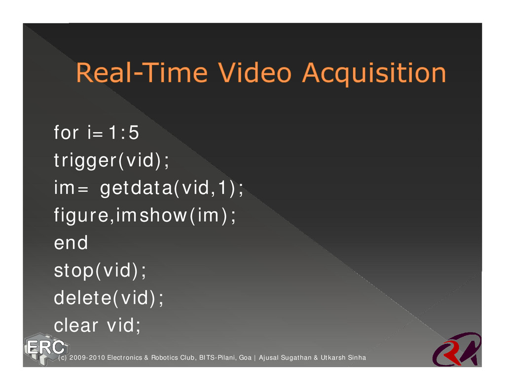
Sugathan & Utkarsh Sinha ž In the above code, object im gets overwritten while execution of each of the interations of the for loop ž To be able to see all the five images, replace im with im(:,:,:,i)
Sugathan & Utkarsh Sinha ž In the above code, object im gets overwritten while execution of each of the interations of the for loop ž To be able to see all the five images, replace im with im(:,:,:,i)
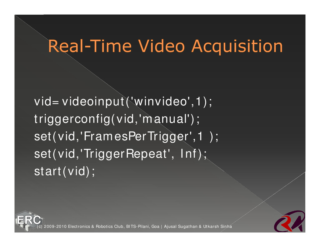
Sugathan & Utkarsh Sinha ž triggerconfig sets the object to manual triggering, since its default triggering is of type immediate ž In immediate triggering, the video is captured as soon as you start the object ‘vid’ ž The captured frames are stored in memory. Getdata function can be used to access these frames ž But in manual triggering, you get the image only when you ‘trigger’ the video
Sugathan & Utkarsh Sinha ž ‘FramesPerTrigger’ decides the number of frames you want to capture each time ‘trigger’ is executed ž TriggerRepeat has to be either equal to the number of frames you want to process in your program or it can be set to Inf ž If set to any positive integer, you will have to ‘start’ the video capture again after trigger is used for those many number of times
Sugathan & Utkarsh Sinha ž Once you are done with acquiring of frames and have stored the images, you can stop the video capture and clear the stored frames from the memory buffer, using following commands: ž >>stop(vid); ž >>delete(vid); ž >>clear vid;
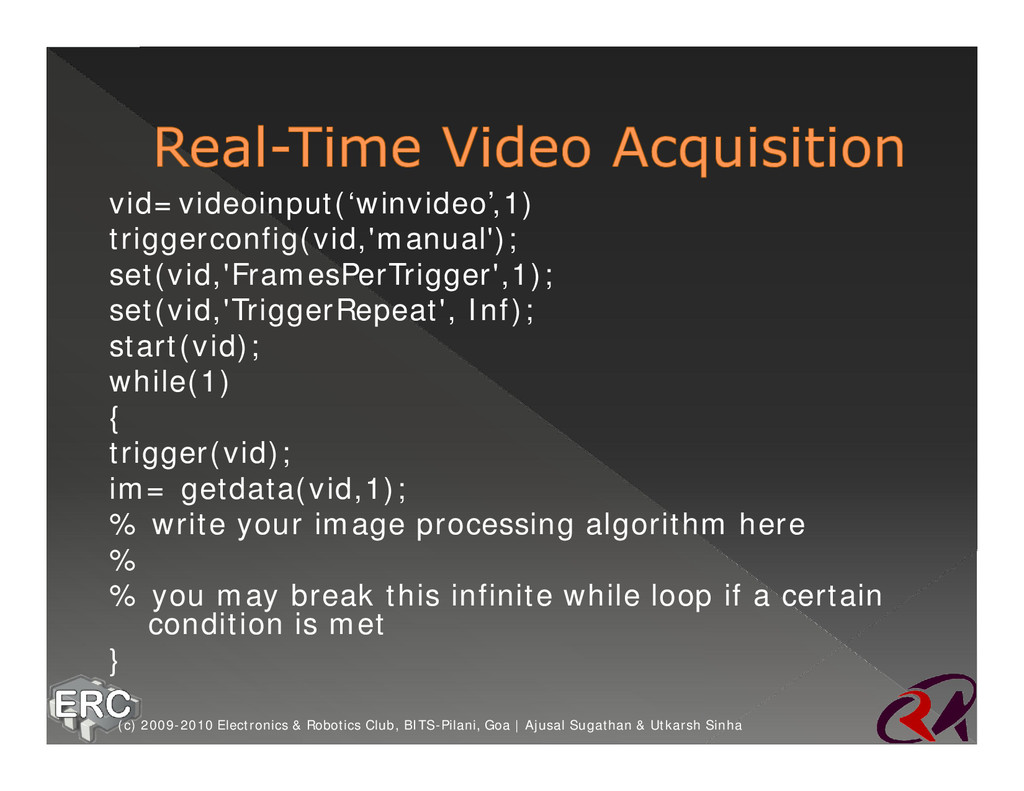
Sugathan & Utkarsh Sinha ž Getsnapshot function returns one image frame and is independent of FramesPerTrigger property ž So if you want to process your images in real-time, this is all you need:
Sugathan & Utkarsh Sinha vid=videoinput(‘winvideo’,1) triggerconfig(vid,'manual'); set(vid,'FramesPerTrigger',1); set(vid,'TriggerRepeat', Inf); start(vid); while(1) { trigger(vid); im= getdata(vid,1); % write your image processing algorithm here % % you may break this infinite while loop if a certain condition is met }
as COM port) and parallel port (also called as printer port or LPT port) of a PC ž MATLAB has an adaptor to access the parallel port (similar to adaptor for image acquisition) (c) 2009-2010 Electronics & Robotics Club, BITS-Pilani, Goa | Ajusal Sugathan & Utkarsh Sinha
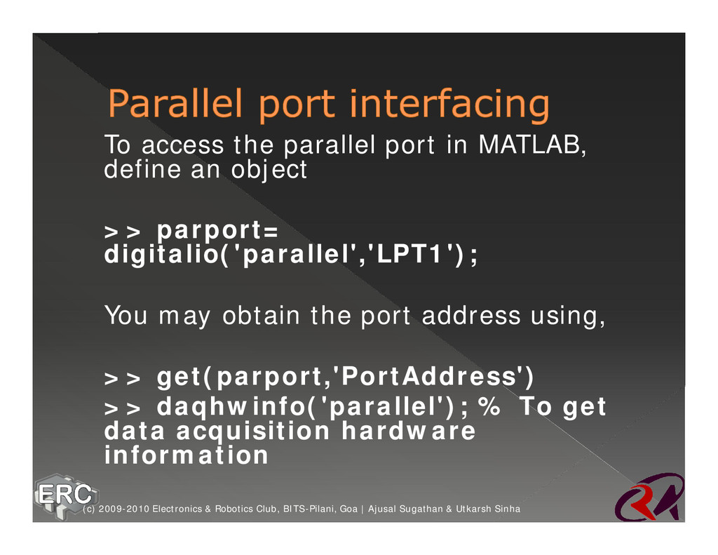
object ž >> parport= digitalio('parallel','LPT1'); ž You may obtain the port address using, ž >> get(parport,'PortAddress') ž >> daqhwinfo('parallel'); % To get data acquisition hardware information (c) 2009-2010 Electronics & Robotics Club, BITS-Pilani, Goa | Ajusal Sugathan & Utkarsh Sinha
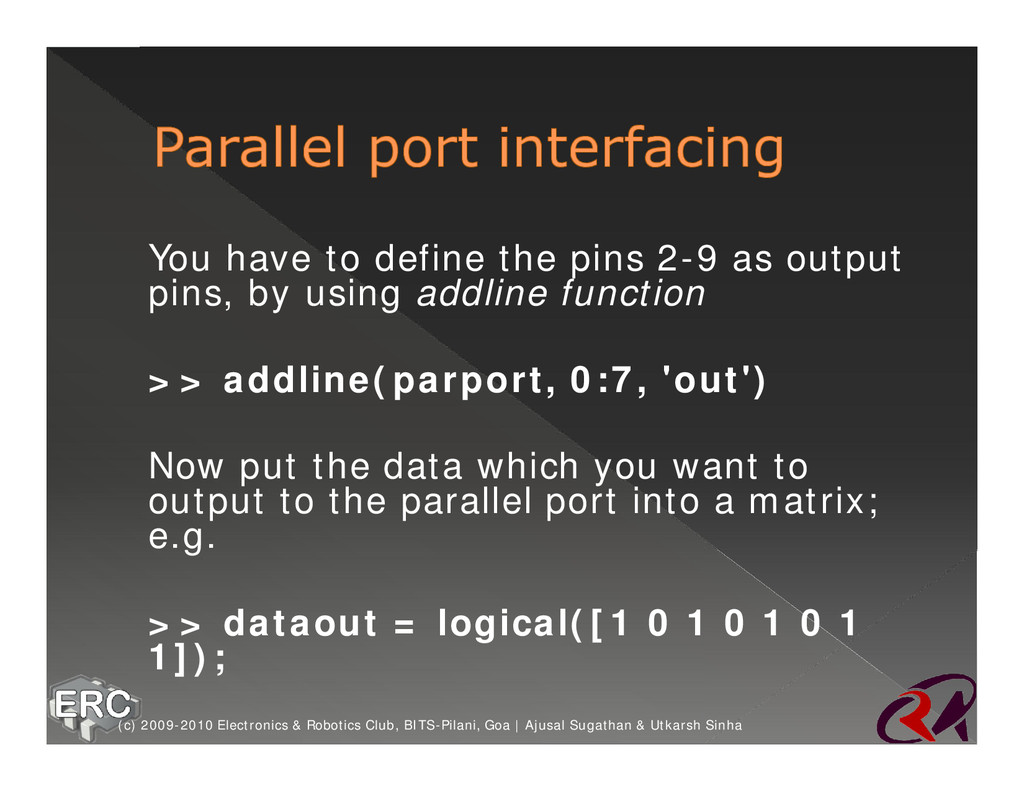
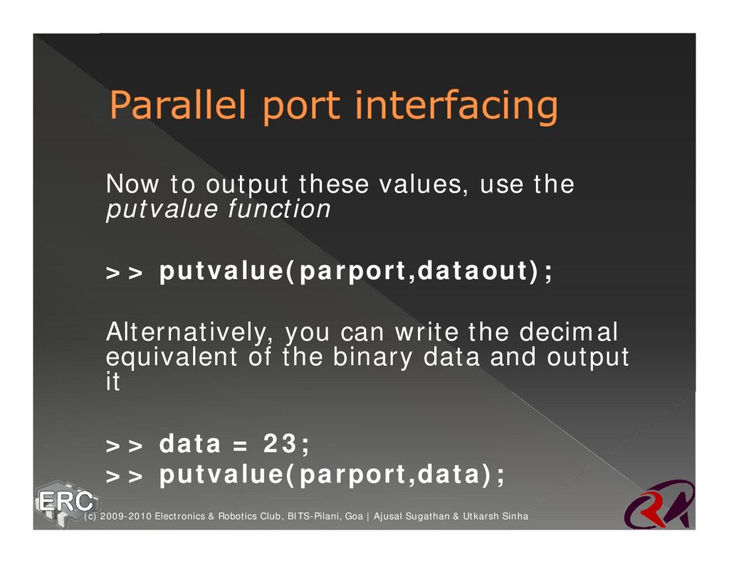
pins, by using addline function ž >> addline(parport, 0:7, 'out') ž Now put the data which you want to output to the parallel port into a matrix; e.g. ž >> dataout = logical([1 0 1 0 1 0 1 1]); (c) 2009-2010 Electronics & Robotics Club, BITS-Pilani, Goa | Ajusal Sugathan & Utkarsh Sinha
ž >> putvalue(parport,dataout); ž Alternatively, you can write the decimal equivalent of the binary data and output it ž >> data = 23; ž >> putvalue(parport,data); (c) 2009-2010 Electronics & Robotics Club, BITS-Pilani, Goa | Ajusal Sugathan & Utkarsh Sinha
to the driver IC for the left and right motors of your robot, and control the left, right, forward and backward motion of the vehicle ž You will need a H-bridge for driving the motor in both clockwise and anti- clockwise directions (c) 2009-2010 Electronics & Robotics Club, BITS-Pilani, Goa | Ajusal Sugathan & Utkarsh Sinha
this library called inpout32 ž Makes your task really simple ž Just follow the instructions that come along, and you’ll be sending data to your robot! (c) 2009-2010 Electronics & Robotics Club, BITS-Pilani, Goa | Ajusal Sugathan & Utkarsh Sinha
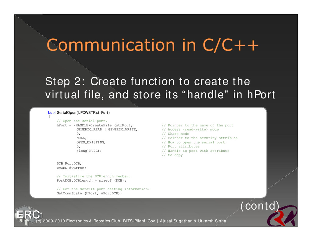
idea is: › Create a virtual file that “represents” the port itself (parallel, serial, etc) › Keep this file open › And keep writing to this file › So, data is automatically send to the desired port (c) 2009-2010 Electronics & Robotics Club, BITS-Pilani, Goa | Ajusal Sugathan & Utkarsh Sinha
and store its “handle” in hPort (contd) bool SerialOpen(LPCWSTR strPort) { // Open the serial port. hPort = (HANDLE)CreateFile (strPort, // Pointer to the name of the port GENERIC_READ | GENERIC_WRITE, // Access (read-write) mode 0, // Share mode NULL, // Pointer to the security attribute OPEN_EXISTING, // How to open the serial port 0, // Port attributes (long)NULL); // Handle to port with attribute // to copy DCB PortDCB; DWORD dwError; // Initialize the DCBlength member. PortDCB.DCBlength = sizeof (DCB); // Get the default port setting information. GetCommState (hPort, &PortDCB); (c) 2009-2010 Electronics & Robotics Club, BITS-Pilani, Goa | Ajusal Sugathan & Utkarsh Sinha
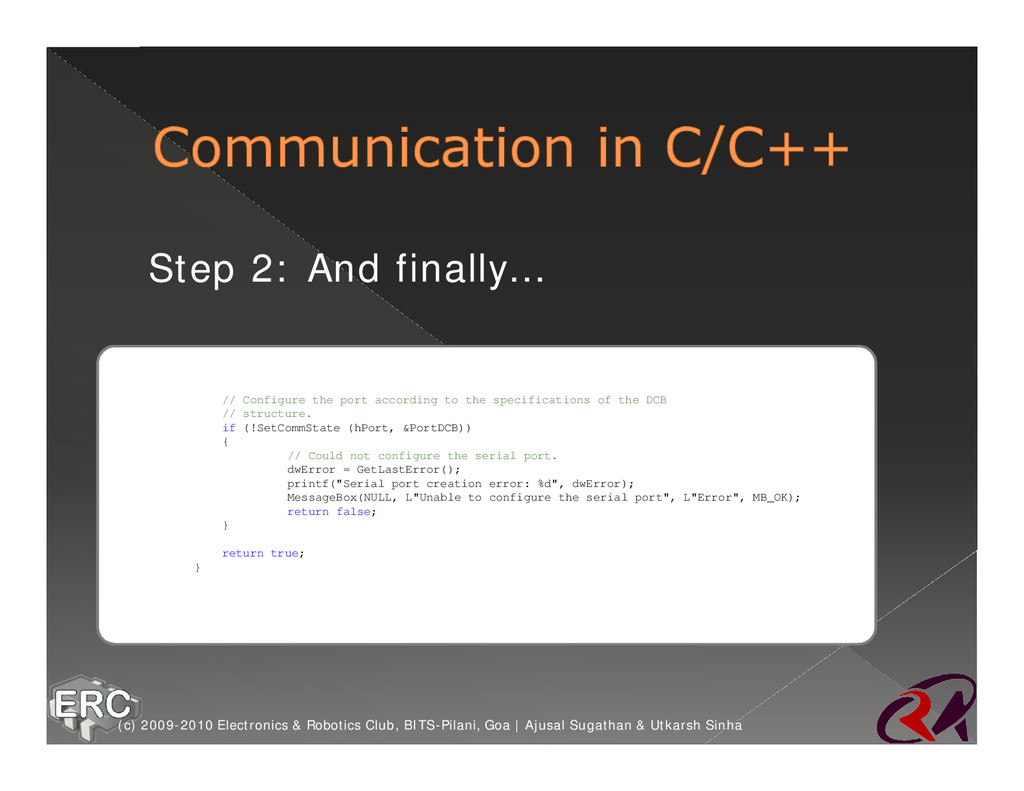
to the specifications of the DCB // structure. if (!SetCommState (hPort, &PortDCB)) { // Could not configure the serial port. dwError = GetLastError(); printf("Serial port creation error: %d", dwError); MessageBox(NULL, L"Unable to configure the serial port", L"Error", MB_OK); return false; } return true; } (c) 2009-2010 Electronics & Robotics Club, BITS-Pilani, Goa | Ajusal Sugathan & Utkarsh Sinha
This function returns a true when the port is created successfully ž If you’re not, replace the “return” statements with “printf”s (c) 2009-2010 Electronics & Robotics Club, BITS-Pilani, Goa | Ajusal Sugathan & Utkarsh Sinha
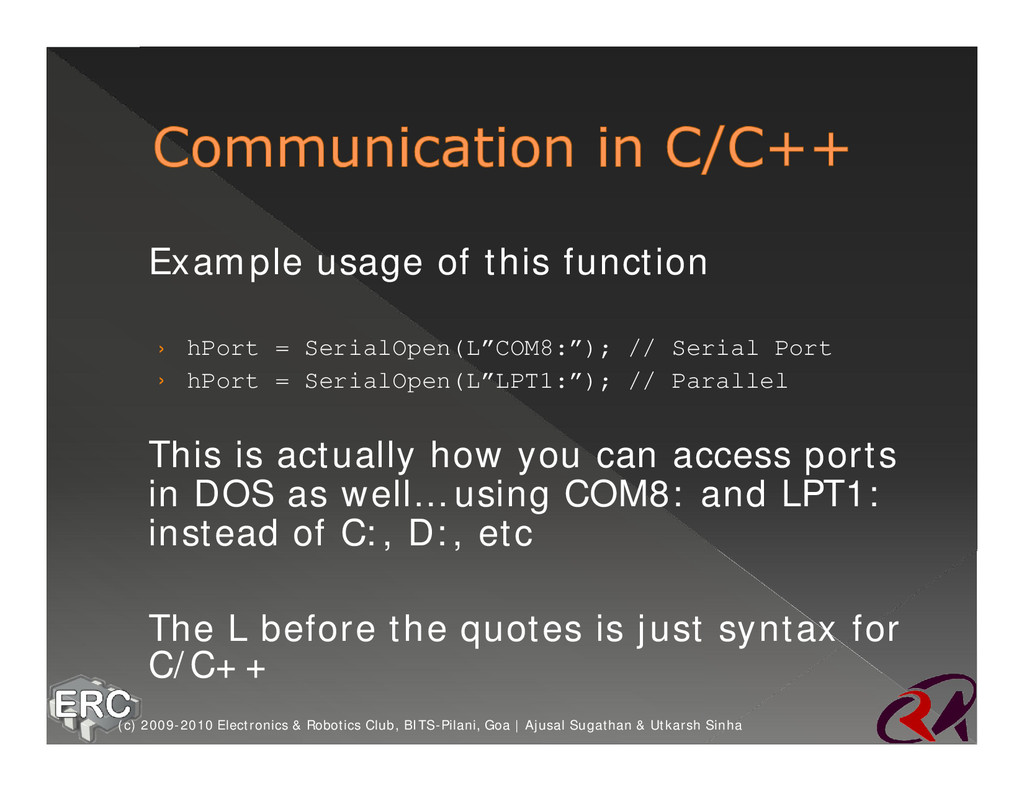
// Serial Port › hPort = SerialOpen(L”LPT1:”); // Parallel ž This is actually how you can access ports in DOS as well… using COM8: and LPT1: instead of C:, D:, etc ž The L before the quotes is just syntax for C/C++ (c) 2009-2010 Electronics & Robotics Club, BITS-Pilani, Goa | Ajusal Sugathan & Utkarsh Sinha
the virtual file we’ve created bool SerialWrite(byte theByte) { // The port wasn't opened if(!hPort) return false; DWORD dwError, dwNumBytesWritten; WriteFile (hPort, // Port handle theByte, // Pointer to the data to write 1, // Number of bytes to write &dwNumBytesWritten, // Pointer to the number of bytes written NULL // Must be NULL ); return true; } (c) 2009-2010 Electronics & Robotics Club, BITS-Pilani, Goa | Ajusal Sugathan & Utkarsh Sinha
a parameter, and it gets written to the port ž Example: SerialWrite(12) (c) 2009-2010 Electronics & Robotics Club, BITS-Pilani, Goa | Ajusal Sugathan & Utkarsh Sinha
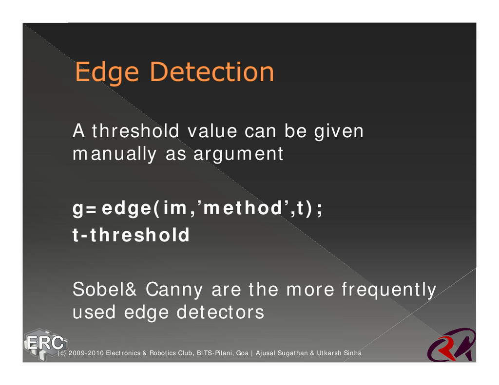
detecting meaningful discontinuities in intensity values ž Done by finding first and second order derivatives of the image ž Also known as gradient of the image (c) 2009-2010 Electronics & Robotics Club, BITS-Pilani, Goa | Ajusal Sugathan & Utkarsh Sinha
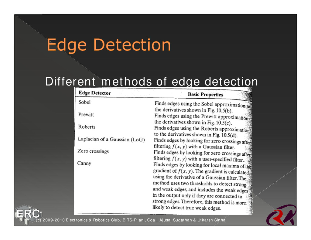
the criteria of derivatives ž An edge detector can be sensitive to horizontal or vertical lines or both ž In detection we try to find out regions where the derivative or gradient is greater than a specified threshold (c) 2009-2010 Electronics & Robotics Club, BITS-Pilani, Goa | Ajusal Sugathan & Utkarsh Sinha
indicate the orientation of the robot ž It should happen with the least number of operations (c) 2009-2010 Electronics & Robotics Club, BITS-Pilani, Goa | Ajusal Sugathan & Utkarsh Sinha
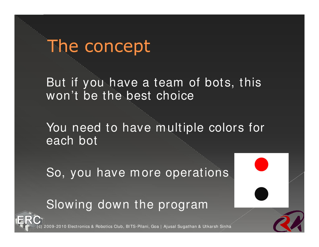
won’t be the best choice ž You need to have multiple colors for each bot ž So, you have more operations ž Slowing down the program (c) 2009-2010 Electronics & Robotics Club, BITS-Pilani, Goa | Ajusal Sugathan & Utkarsh Sinha
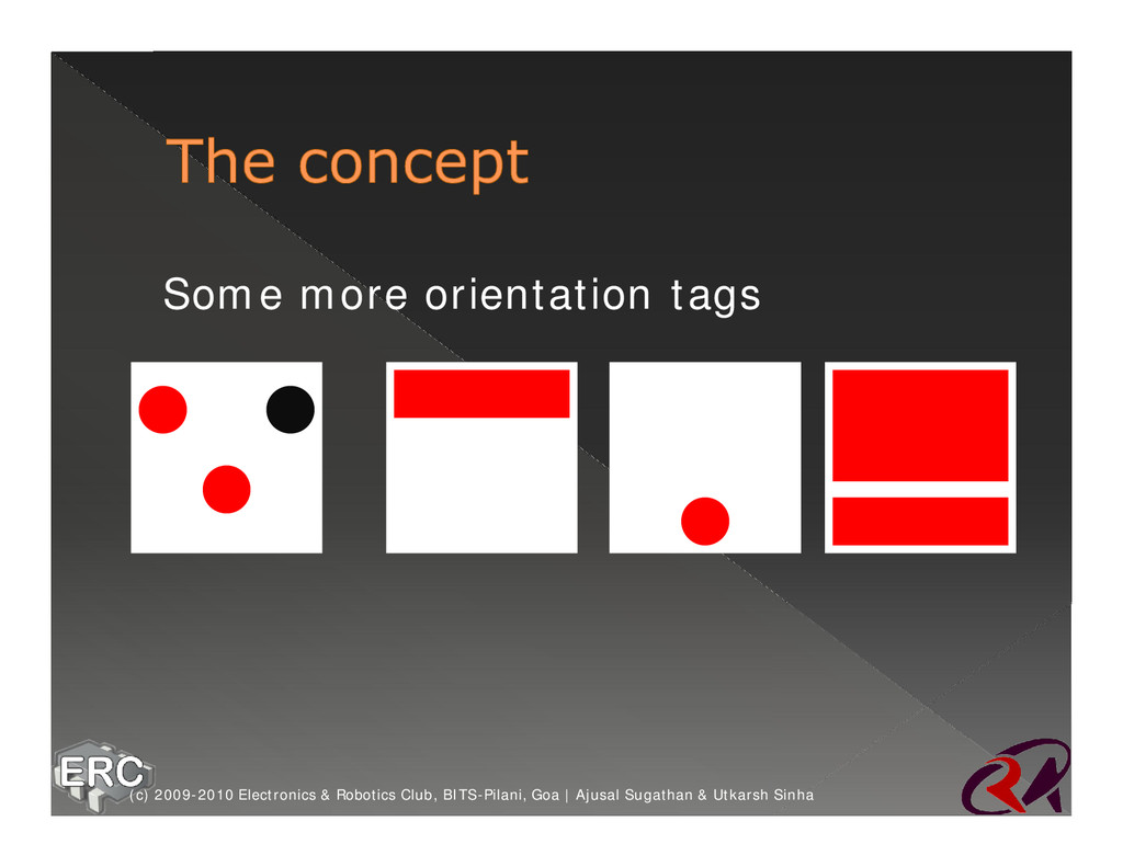
The asymmetry helps distinguish between multiple bots, with just two colors (c) 2009-2010 Electronics & Robotics Club, BITS-Pilani, Goa | Ajusal Sugathan & Utkarsh Sinha
› Using OpenCV’s built in libraries › Using some 3rd party capturing library (c) 2009-2010 Electronics & Robotics Club, BITS-Pilani, Goa | Ajusal Sugathan & Utkarsh Sinha
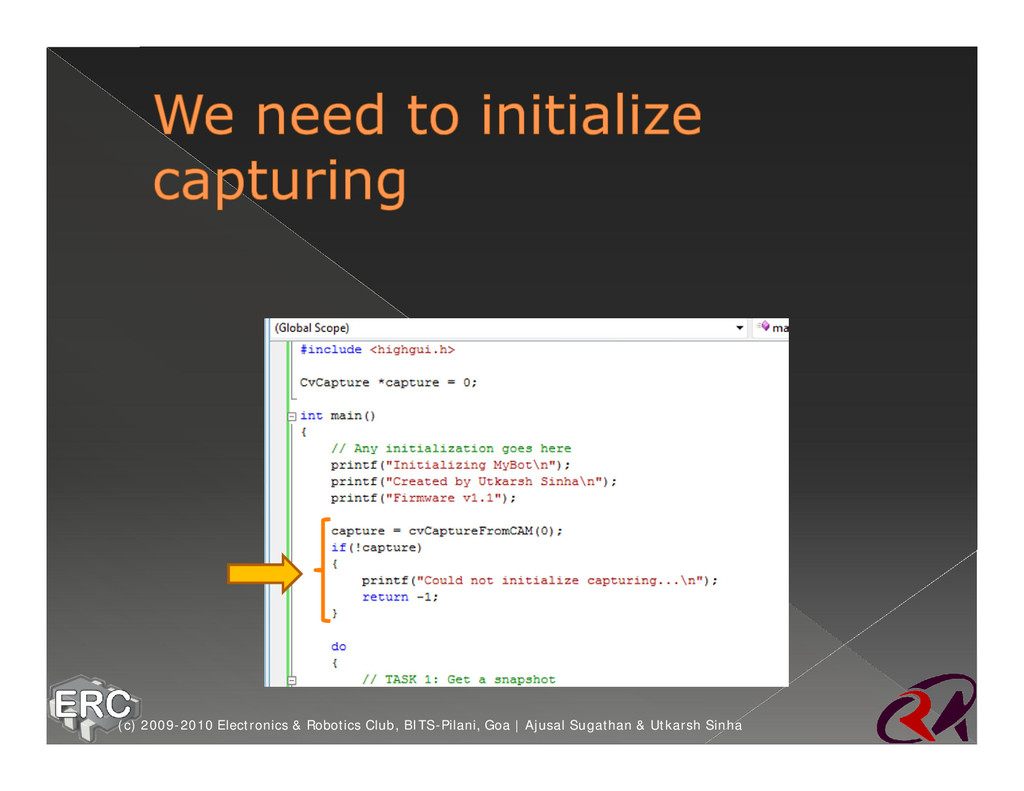
when you have multiple cameras attached to the same machine (like in stereo vision) ž Then we check if we were able to get exclusive control of the camera. If not, quit. (c) 2009-2010 Electronics & Robotics Club, BITS-Pilani, Goa | Ajusal Sugathan & Utkarsh Sinha
going on within the program, what decisions are taken, etc (c) 2009-2010 Electronics & Robotics Club, BITS-Pilani, Goa | Ajusal Sugathan & Utkarsh Sinha
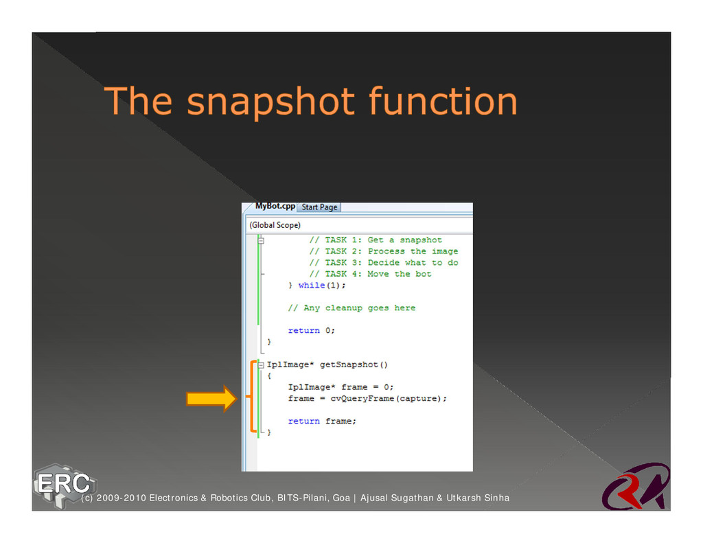
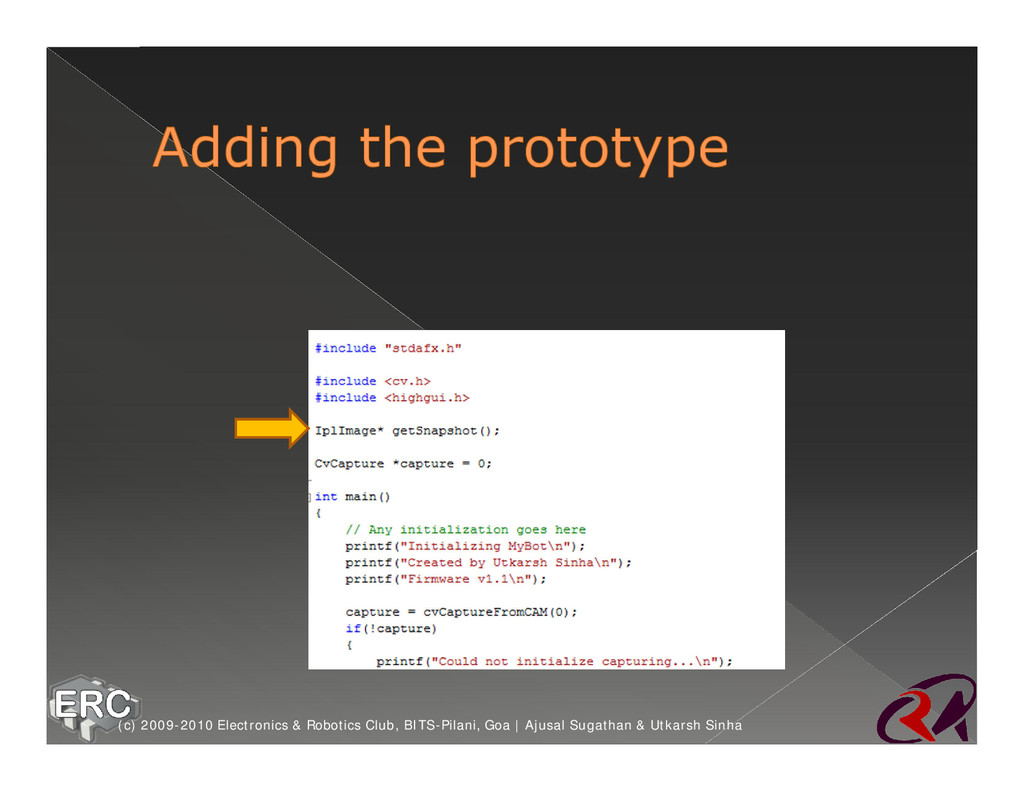
will use the CvCapture structure to tap into the camera’s stream ž It will return a single frame as an IplImage structure ž Scroll down, and add the function (c) 2009-2010 Electronics & Robotics Club, BITS-Pilani, Goa | Ajusal Sugathan & Utkarsh Sinha
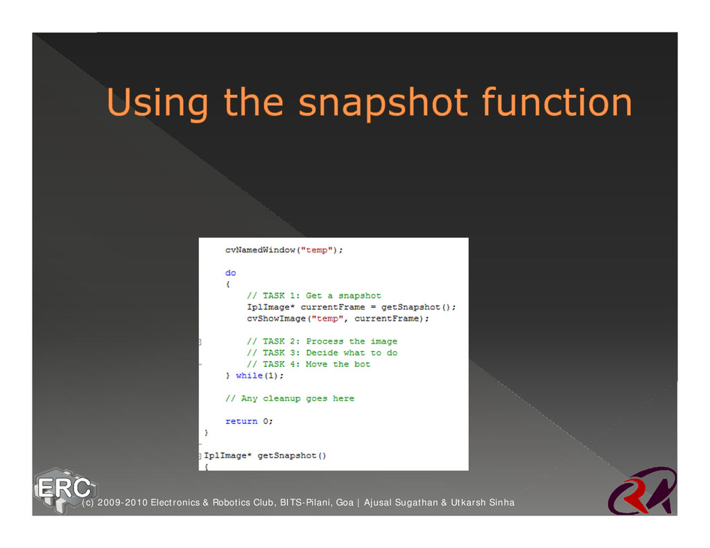
we had created ž Because the getSnapshot() function returns a single frame, we need to take snaps regularly ž So it goes into the do…while loop (c) 2009-2010 Electronics & Robotics Club, BITS-Pilani, Goa | Ajusal Sugathan & Utkarsh Sinha
get an error ž getSnapshot() comes “after” the main function ž So the compiler doesn’t know if it exists ž Hence we need the so called “prototype” (c) 2009-2010 Electronics & Robotics Club, BITS-Pilani, Goa | Ajusal Sugathan & Utkarsh Sinha
DirectX is a much bigger library and supports almost all cameras that exist (c) 2009-2010 Electronics & Robotics Club, BITS-Pilani, Goa | Ajusal Sugathan & Utkarsh Sinha
Visual Studio where to find the required external files ž So we follow steps similar to the OpenCV ones. ž The VideoInput package comes with lots of sample code, so you shouldn’t have much problem (c) 2009-2010 Electronics & Robotics Club, BITS-Pilani, Goa | Ajusal Sugathan & Utkarsh Sinha
as quickly as possible ž So we use a loop of some kind (usually a do…while) ž Within the loop, you do the following tasks: (c) 2009-2010 Electronics & Robotics Club, BITS-Pilani, Goa | Ajusal Sugathan & Utkarsh Sinha
of each object in the arena ž Use moments, contours, or anything else ž Thresholding, morphology, etc are helpful here (c) 2009-2010 Electronics & Robotics Club, BITS-Pilani, Goa | Ajusal Sugathan & Utkarsh Sinha
what to do next ž Bot: Should I go to the red ball because it’s the closest? Or should I go to the green ball because it has the maximum number of points (c) 2009-2010 Electronics & Robotics Club, BITS-Pilani, Goa | Ajusal Sugathan & Utkarsh Sinha
move ž You must include feedback in this step itself (maybe another do…while loop) (c) 2009-2010 Electronics & Robotics Club, BITS-Pilani, Goa | Ajusal Sugathan & Utkarsh Sinha
is necessary (have all the balls been potted?) If required, only then go to Task 1 › Blindly go to Task 1 (the decision module will tell the bot when to stop) ž Both options are good enough (c) 2009-2010 Electronics & Robotics Club, BITS-Pilani, Goa | Ajusal Sugathan & Utkarsh Sinha
won’t go into code. Just high level logic on how to go about it (c) 2009-2010 Electronics & Robotics Club, BITS-Pilani, Goa | Ajusal Sugathan & Utkarsh Sinha
Everything is measure in terms of pixels: distances, coordinates, etc ž Angles are usually represented in radians (cos, sin, etc work well with radians) (c) 2009-2010 Electronics & Robotics Club, BITS-Pilani, Goa | Ajusal Sugathan & Utkarsh Sinha
And you need to stick with it throughout your code ž Here’s a coordinate system I used several times (c) 2009-2010 Electronics & Robotics Club, BITS-Pilani, Goa | Ajusal Sugathan & Utkarsh Sinha
system ž In particular, you must make sure all your angle calculations are consistent ž And that they cycle through 359-1 degrees perfectly (c) 2009-2010 Electronics & Robotics Club, BITS-Pilani, Goa | Ajusal Sugathan & Utkarsh Sinha
the coordinate system › This would be the very basic feedback function › Within this function, you have a loop › This loop keeps running as long as the bot isn’t oriented at angle degrees › You’ll take snapshots within this function as well (c) 2009-2010 Electronics & Robotics Club, BITS-Pilani, Goa | Ajusal Sugathan & Utkarsh Sinha
coordinates (x,y) in the image › If required, you can also put a call to TurnBotToAngle (to orient the bot to move) › Again, there’s a loop which keeps running until the bot reaches the desired position › And you’ll need to take multiple snapshots to check where the bot actually is (c) 2009-2010 Electronics & Robotics Club, BITS-Pilani, Goa | Ajusal Sugathan & Utkarsh Sinha
you say TurnBotToAngle(30), it’s very unlikely that the bot will orient to exactly 30 degrees ž A range, say 28-32 should be good enough (c) 2009-2010 Electronics & Robotics Club, BITS-Pilani, Goa | Ajusal Sugathan & Utkarsh Sinha
are in the image, in terms of pixels ž We have no idea how they relate to physical distances and angles ž But we’re sure that they are proportional to physical distances and angles (c) 2009-2010 Electronics & Robotics Club, BITS-Pilani, Goa | Ajusal Sugathan & Utkarsh Sinha
out physical distances ž For example, 5pixels = 3cm ž This is very much possible, but of no use for our purposes! (c) 2009-2010 Electronics & Robotics Club, BITS-Pilani, Goa | Ajusal Sugathan & Utkarsh Sinha
you don’t need to know OOPs to use them. ž They really simplify your work, and even make the code more readable (c) 2009-2010 Electronics & Robotics Club, BITS-Pilani, Goa | Ajusal Sugathan & Utkarsh Sinha
then checks if the angle is correct or not, etc ž Try working on something which checks the bot’s angle without stopping the bot (c) 2009-2010 Electronics & Robotics Club, BITS-Pilani, Goa | Ajusal Sugathan & Utkarsh Sinha
use… so thresholding in YUV itself will eliminate processing time consumed by YUV to RGB conversion) (c) 2009-2010 Electronics & Robotics Club, BITS-Pilani, Goa | Ajusal Sugathan & Utkarsh Sinha
position might be calculated as different for different frames. ž If you use Kalman filters, you can “smooth out” the position data and get precise positioning and angle data (c) 2009-2010 Electronics & Robotics Club, BITS-Pilani, Goa | Ajusal Sugathan & Utkarsh Sinha
based competitions ž All this knowledge can even serve as a start point for further studies in image processing ž Enjoy! (c) 2009-2010 Electronics & Robotics Club, BITS-Pilani, Goa | Ajusal Sugathan & Utkarsh Sinha
![#include <cv.h> #include <highgui.h> int main() { IplImage* imgRed[25]; IplImage*](https://files.speakerdeck.com/presentations/be8942f0f6c60131fa0836a487f750f5/slide_265.jpg)
![IplImage* imgBlue[25]; for(int i=0;i<25;i++) { IplImage* img; char filename[150]; sprintf(filename,](https://files.speakerdeck.com/presentations/be8942f0f6c60131fa0836a487f750f5/slide_266.jpg)
![img = cvLoadImage(filename); imgRed[i] = cvCreateImage(cvGetSize(img), 8, 1); imgGreen[i] =](https://files.speakerdeck.com/presentations/be8942f0f6c60131fa0836a487f750f5/slide_267.jpg)
![imgBlue[i] = cvCreateImage(cvGetSize(img), 8, 1); cvSplit(img, imgBlue[i], imgGreen[i], imgRed[i], NULL);](https://files.speakerdeck.com/presentations/be8942f0f6c60131fa0836a487f750f5/slide_268.jpg)
![CvSize imgSize = cvGetSize(imgRed[0]); IplImage* imgResultRed = cvCreateImage(imgSize, 8, 1);](https://files.speakerdeck.com/presentations/be8942f0f6c60131fa0836a487f750f5/slide_270.jpg)
![for(int i=0;i<25;i++) { theSumRed+=cvGetReal2D(imgRed[i], y, x); theSumGreen+=cvGetReal2D(imgGreen[i], y, x); theSumBlue+=cvGetReal2D(imgBlue[i],](https://files.speakerdeck.com/presentations/be8942f0f6c60131fa0836a487f750f5/slide_273.jpg)
![function [temp] = ht(im,level1,level2) s=size(im); temp=im; for i=1:s(1,1) for j=1:s(1,2)](https://files.speakerdeck.com/presentations/be8942f0f6c60131fa0836a487f750f5/slide_339.jpg)
![if(result->total==4) { CvPoint *pt[4]; for(int i=0;i<4;i++) pt[i] = (CvPoint*)cvGetSeqElem(result, i);](https://files.speakerdeck.com/presentations/be8942f0f6c60131fa0836a487f750f5/slide_378.jpg)
![ž General Command in MATLAB ž [g t] = edge(im,’method’,parameters);](https://files.speakerdeck.com/presentations/be8942f0f6c60131fa0836a487f750f5/slide_442.jpg)