Electronegativity

Transcript

1. electronegativity from a high school concept to a research tool Łukasz Mentel October 15, 2015 Catalysis Group, UiO
2. Conceptual chemistry 1
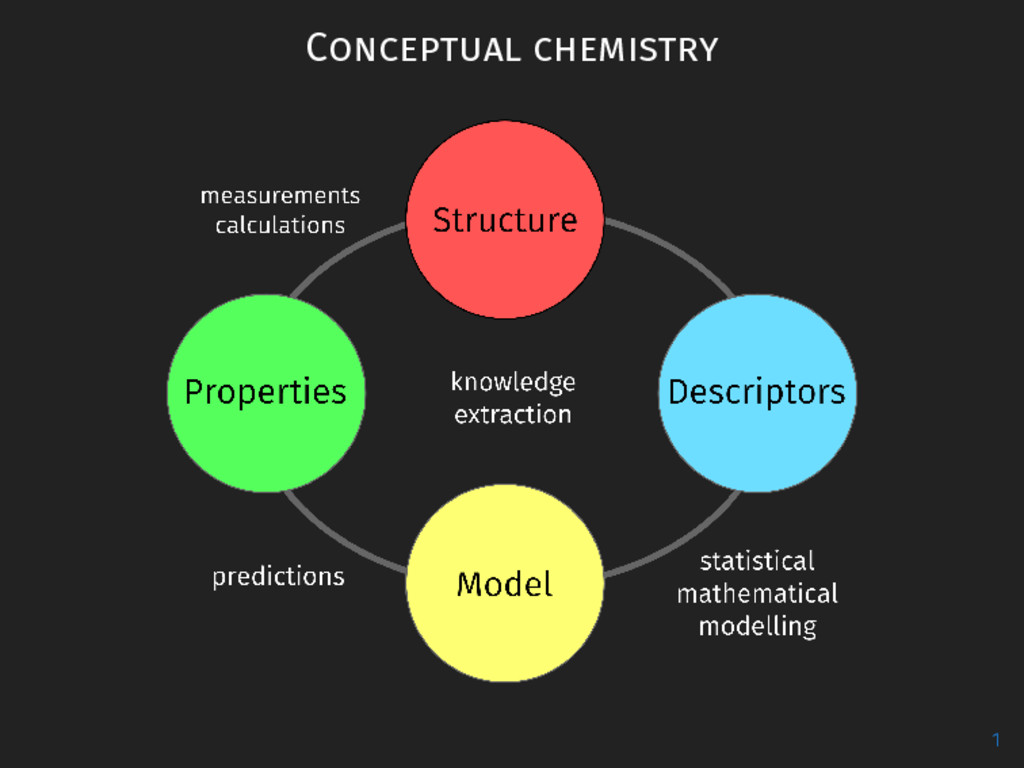
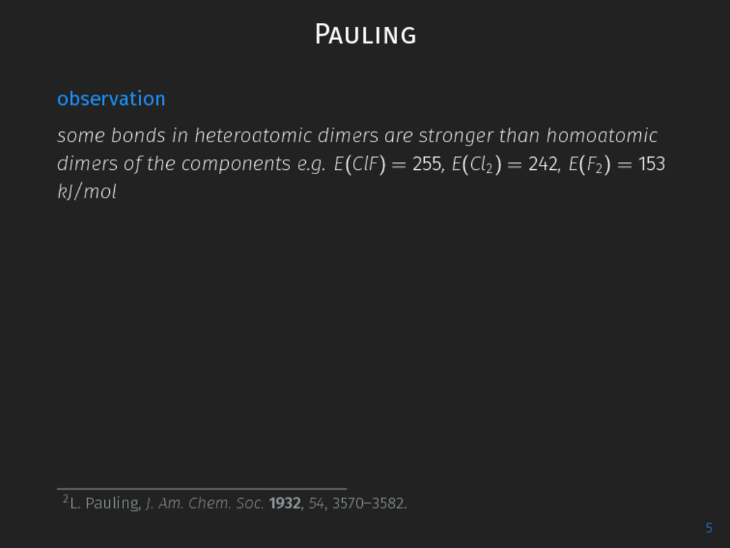
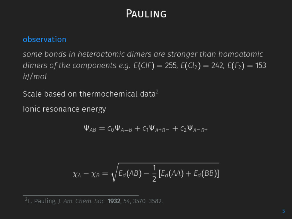
3. Towards models qualitative to be able to understand and rationalize properties and reactivities of atoms, isolated molecules, liquids and solids in terms of a single number characteristics of each systems components quantitative to be able to quantify the similarities and differences between systems and their properties and make predictions 2
4. Electronegativity (χ) the power of an atom in a molecule to attract electrons to itself — L. Pauling, The Nature of Chemical Bond (1939) 3
5. A bit of history Important steps towards the modern concept of electronegativity1 ∙ 1749, 1751 P. Macquer, chemical affinity of similar bodies 1W. B. Jensen, J. Chem. Educ. 1996, 73, 11, W. B. Jensen, J. Chem. Educ. 2003, 80, 279. Periodic Table: D. Mendeleev 1869, L. Meyer 1870 4
6. A bit of history Important steps towards the modern concept of electronegativity1 ∙ 1749, 1751 P. Macquer, chemical affinity of similar bodies ∙ 1789 A. Fourcroy, affinity of different bodies 1W. B. Jensen, J. Chem. Educ. 1996, 73, 11, W. B. Jensen, J. Chem. Educ. 2003, 80, 279. Periodic Table: D. Mendeleev 1869, L. Meyer 1870 4
7. A bit of history Important steps towards the modern concept of electronegativity1 ∙ 1749, 1751 P. Macquer, chemical affinity of similar bodies ∙ 1789 A. Fourcroy, affinity of different bodies ∙ 1809 A. Avogadro, relative scale of oxygenicity, acid-base antagonism grows with difference in oxygenicity 1W. B. Jensen, J. Chem. Educ. 1996, 73, 11, W. B. Jensen, J. Chem. Educ. 2003, 80, 279. Periodic Table: D. Mendeleev 1869, L. Meyer 1870 4
8. A bit of history Important steps towards the modern concept of electronegativity1 ∙ 1749, 1751 P. Macquer, chemical affinity of similar bodies ∙ 1789 A. Fourcroy, affinity of different bodies ∙ 1809 A. Avogadro, relative scale of oxygenicity, acid-base antagonism grows with difference in oxygenicity ∙ 1822 J. J. Berzelius, electronegativity, acid-alkaline antagonism becomes electronegative-electropositive 1W. B. Jensen, J. Chem. Educ. 1996, 73, 11, W. B. Jensen, J. Chem. Educ. 2003, 80, 279. Periodic Table: D. Mendeleev 1869, L. Meyer 1870 4
9. A bit of history Important steps towards the modern concept of electronegativity1 ∙ 1749, 1751 P. Macquer, chemical affinity of similar bodies ∙ 1789 A. Fourcroy, affinity of different bodies ∙ 1809 A. Avogadro, relative scale of oxygenicity, acid-base antagonism grows with difference in oxygenicity ∙ 1822 J. J. Berzelius, electronegativity, acid-alkaline antagonism becomes electronegative-electropositive ∙ 1870, G. Baker, augmented (Berzelius) electronegativity scale 1W. B. Jensen, J. Chem. Educ. 1996, 73, 11, W. B. Jensen, J. Chem. Educ. 2003, 80, 279. Periodic Table: D. Mendeleev 1869, L. Meyer 1870 4
10. A bit of history Important steps towards the modern concept of electronegativity1 ∙ 1749, 1751 P. Macquer, chemical affinity of similar bodies ∙ 1789 A. Fourcroy, affinity of different bodies ∙ 1809 A. Avogadro, relative scale of oxygenicity, acid-base antagonism grows with difference in oxygenicity ∙ 1822 J. J. Berzelius, electronegativity, acid-alkaline antagonism becomes electronegative-electropositive ∙ 1870, G. Baker, augmented (Berzelius) electronegativity scale ∙ 1888, L. Meyer, electronegativity and periodicity 1W. B. Jensen, J. Chem. Educ. 1996, 73, 11, W. B. Jensen, J. Chem. Educ. 2003, 80, 279. Periodic Table: D. Mendeleev 1869, L. Meyer 1870 4
11. A bit of history Important steps towards the modern concept of electronegativity1 ∙ 1749, 1751 P. Macquer, chemical affinity of similar bodies ∙ 1789 A. Fourcroy, affinity of different bodies ∙ 1809 A. Avogadro, relative scale of oxygenicity, acid-base antagonism grows with difference in oxygenicity ∙ 1822 J. J. Berzelius, electronegativity, acid-alkaline antagonism becomes electronegative-electropositive ∙ 1870, G. Baker, augmented (Berzelius) electronegativity scale ∙ 1888, L. Meyer, electronegativity and periodicity ∙ 1899, J. van’t Hoff, electronegativity and reaction enthalpies 1W. B. Jensen, J. Chem. Educ. 1996, 73, 11, W. B. Jensen, J. Chem. Educ. 2003, 80, 279. Periodic Table: D. Mendeleev 1869, L. Meyer 1870 4
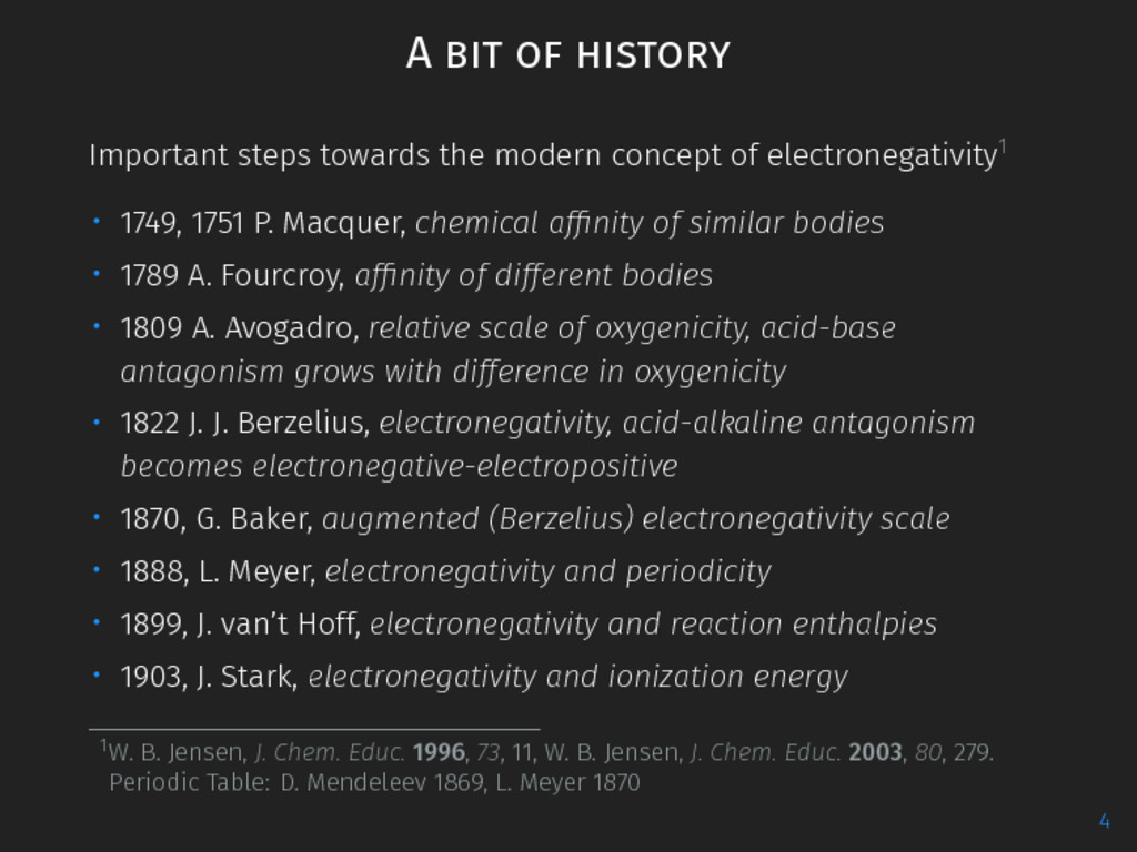
12. A bit of history Important steps towards the modern concept of electronegativity1 ∙ 1749, 1751 P. Macquer, chemical affinity of similar bodies ∙ 1789 A. Fourcroy, affinity of different bodies ∙ 1809 A. Avogadro, relative scale of oxygenicity, acid-base antagonism grows with difference in oxygenicity ∙ 1822 J. J. Berzelius, electronegativity, acid-alkaline antagonism becomes electronegative-electropositive ∙ 1870, G. Baker, augmented (Berzelius) electronegativity scale ∙ 1888, L. Meyer, electronegativity and periodicity ∙ 1899, J. van’t Hoff, electronegativity and reaction enthalpies ∙ 1903, J. Stark, electronegativity and ionization energy 1W. B. Jensen, J. Chem. Educ. 1996, 73, 11, W. B. Jensen, J. Chem. Educ. 2003, 80, 279. Periodic Table: D. Mendeleev 1869, L. Meyer 1870 4
13. Pauling observation some bonds in heteroatomic dimers are stronger than homoatomic dimers of the components e.g. E(ClF) = 255, E(Cl2 ) = 242, E(F2 ) = 153 kJ/mol 2L. Pauling, J. Am. Chem. Soc. 1932, 54, 3570–3582. 5
14. Pauling observation some bonds in heteroatomic dimers are stronger than homoatomic dimers of the components e.g. E(ClF) = 255, E(Cl2 ) = 242, E(F2 ) = 153 kJ/mol Scale based on thermochemical data2 Ionic resonance energy ΨAB = c0 ΨA−B + c1 ΨA+B− + c2 ΨA−B+ χA − χB = Ed (AB) − 1 2 [Ed (AA) + Ed (BB)] 2L. Pauling, J. Am. Chem. Soc. 1932, 54, 3570–3582. 5
16. Mulliken Considering the wave function for ionic and covalent bond Mulliken suggested3 χM = IP + EA 2 Ionization energy/potential A(g) → A+(g) + e−(g) IP = E(A+, g) − E(A, g) Electron affinity A(g) + e−(g) → A−(g) EA = E(A, g) − E(A−, g) 3R. S. Mulliken, J. Chem. Phys. 1934, 2, 782. 7
17. Pauling vs Mulliken 8
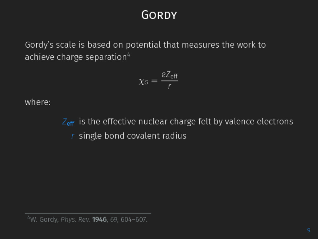
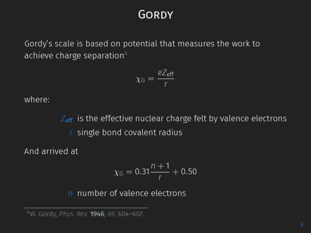
18. Gordy Gordy’s scale is based on potential that measures the work to achieve charge separation4 χG = eZeff r where: Zeff is the effective nuclear charge felt by valence electrons r single bond covalent radius 4W. Gordy, Phys. Rev. 1946, 69, 604–607. 9
19. Gordy Gordy’s scale is based on potential that measures the work to achieve charge separation4 χG = eZeff r where: Zeff is the effective nuclear charge felt by valence electrons r single bond covalent radius And arrived at χG = 0.31 n + 1 r + 0.50 n number of valence electrons 4W. Gordy, Phys. Rev. 1946, 69, 604–607. 9
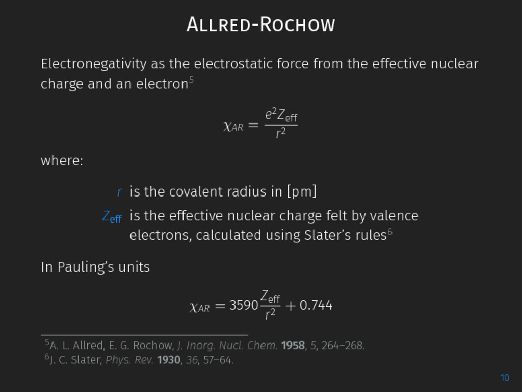
20. Allred-Rochow Electronegativity as the electrostatic force from the effective nuclear charge and an electron5 χAR = e2Zeff r2 where: r is the covalent radius in [pm] Zeff is the effective nuclear charge felt by valence electrons, calculated using Slater’s rules6 In Pauling’s units χAR = 3590 Zeff r2 + 0.744 5A. L. Allred, E. G. Rochow, J. Inorg. Nucl. Chem. 1958, 5, 264–268. 6J. C. Slater, Phys. Rev. 1930, 36, 57–64. 10
21. Allen Allen defined his scale in terms of configurational energy7 χA = ns εs + np εp ns + np χA = ns εs + nd εd ns + nd where: ns , np , nd numbers of s, p and d valence electrons εs , εp , εd multiplet averaged one-electron energies [Ry] In Pauling’s units χA = 2.30016 ns εs + np εp ns + np 7L. C. Allen, J. Am. Chem. Soc. 1989, 111, 9003–9014, J. B. Mann et al., J. Am. Chem. Soc. 2000, 122, 5132–5137, J. B. Mann et al., J. Am. Chem. Soc. 2000, 122, 2780–2783. 11
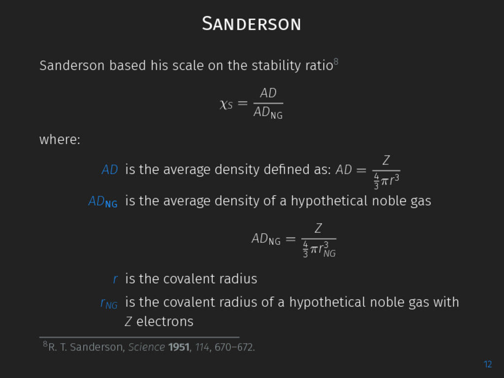
22. Sanderson Sanderson based his scale on the stability ratio8 χS = AD ADNG where: AD is the average density defined as: AD = Z 4 3 πr3 ADNG is the average density of a hypothetical noble gas ADNG = Z 4 3 πr3 NG r is the covalent radius rNG is the covalent radius of a hypothetical noble gas with Z electrons 8R. T. Sanderson, Science 1951, 114, 670–672. 12
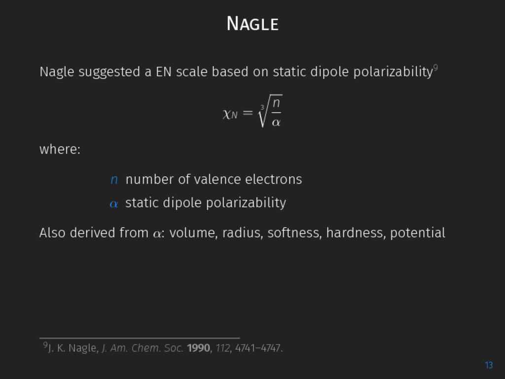
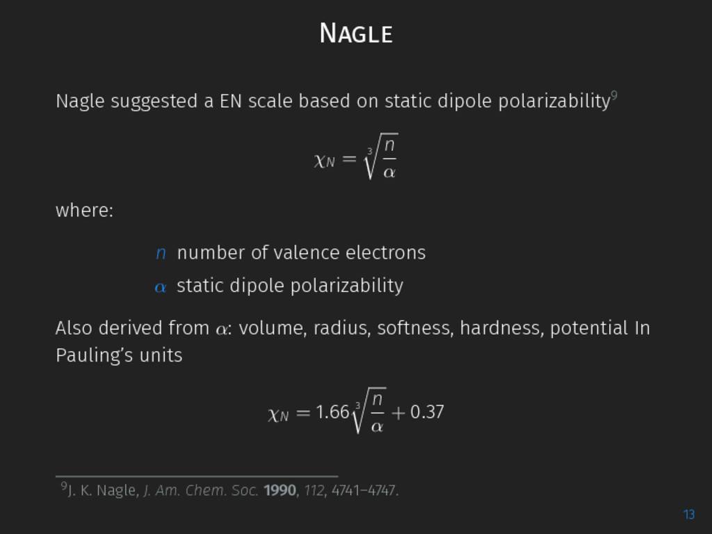
23. Nagle Nagle suggested a EN scale based on static dipole polarizability9 χN = 3 n α where: n number of valence electrons α static dipole polarizability Also derived from α: volume, radius, softness, hardness, potential 9J. K. Nagle, J. Am. Chem. Soc. 1990, 112, 4741–4747. 13
24. Nagle Nagle suggested a EN scale based on static dipole polarizability9 χN = 3 n α where: n number of valence electrons α static dipole polarizability Also derived from α: volume, radius, softness, hardness, potential In Pauling’s units χN = 1.66 3 n α + 0.37 9J. K. Nagle, J. Am. Chem. Soc. 1990, 112, 4741–4747. 13
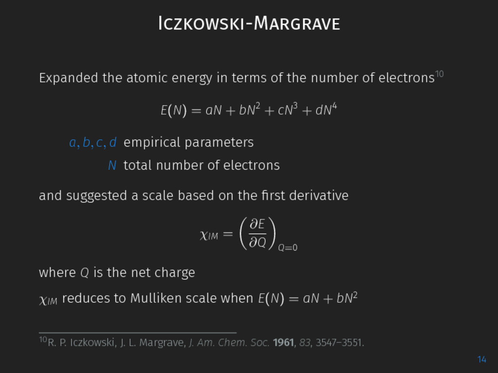
25. Iczkowski-Margrave Expanded the atomic energy in terms of the number of electrons10 E(N) = aN + bN2 + cN3 + dN4 a, b, c, d empirical parameters N total number of electrons and suggested a scale based on the first derivative χIM = ∂E ∂Q Q=0 where Q is the net charge χIM reduces to Mulliken scale when E(N) = aN + bN2 10R. P. Iczkowski, J. L. Margrave, J. Am. Chem. Soc. 1961, 83, 3547–3551. 14
26. Politzer Average local ionization energy11 I(r) = i ρi (r) |εi | ρ(r) where sum runs over all occupied orbitals and: ρi (r) is the electronic density of orbital φi (r) εi energy of the orbital φi (r) ρ(r) total electronic density r is usually taken as 0.001 au contour 11P. Politzer et al., J. Chem. Theory Comput. 2011, 7, 377–384. 15
27. why bother Qualitative and quantitative models based on electronegativity ∙ bond length ∙ bond strength ∙ charges ∙ group electronegativity ∙ reaction mechanisms electrophilic/nucleophilic attack direction ∙ Gibbs free energy12 ∙ superconductivity13 12P. Vieillard, Clays and Clay Minerals, 48, 459–473. 13Q.-G. Luo, R.-y. Wang, J. Phys. Chem. Solids 1987, 48, 425–430, S. Ichikawa, J. Phys. Chem. Solids 1989, 50, 931–934, R. Jayaprakash, J. Shanker, J. Phys. Chem. Solids 1993, 54, 365–369. 16
28. Challenges ∙ electronegativity is NOT an observable ∙ different scales treat EN as an intrinsic property of a element OR a property that describes an atom in molecular environment ”atom in molecule” ∙ although the scales of EN are related by a linear transformation there are differences ∙ no agreement on how to incorporate the state of the atom in the scales ∙ no consensus even about the unit of EN 17
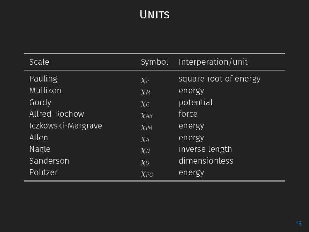
29. Units Scale Symbol Interperation/unit Pauling χP square root of energy Mulliken χM energy Gordy χG potential Allred-Rochow χAR force Iczkowski-Margrave χIM energy Allen χA energy Nagle χN inverse length Sanderson χS dimensionless Politzer χPO energy 18
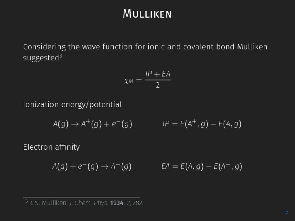
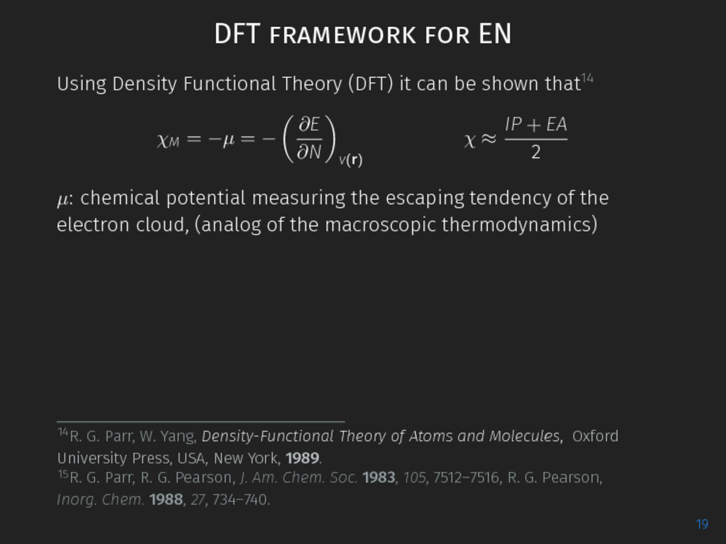
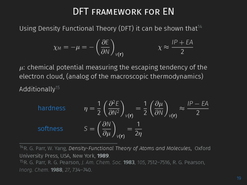
30. DFT framework for EN Using Density Functional Theory (DFT) it can be shown that14 χM = −µ = − ∂E ∂N v(r) χ ≈ IP + EA 2 µ: chemical potential measuring the escaping tendency of the electron cloud, (analog of the macroscopic thermodynamics) 14R. G. Parr, W. Yang, Density-Functional Theory of Atoms and Molecules, Oxford University Press, USA, New York, 1989. 15R. G. Parr, R. G. Pearson, J. Am. Chem. Soc. 1983, 105, 7512–7516, R. G. Pearson, Inorg. Chem. 1988, 27, 734–740. 19
31. DFT framework for EN Using Density Functional Theory (DFT) it can be shown that14 χM = −µ = − ∂E ∂N v(r) χ ≈ IP + EA 2 µ: chemical potential measuring the escaping tendency of the electron cloud, (analog of the macroscopic thermodynamics) Additionally15 hardness η = 1 2 ∂2E ∂N2 v(r) = 1 2 ∂µ ∂N v(r) ≈ IP − EA 2 softness S = ∂N ∂µ v(r) = 1 2η 14R. G. Parr, W. Yang, Density-Functional Theory of Atoms and Molecules, Oxford University Press, USA, New York, 1989. 15R. G. Parr, R. G. Pearson, J. Am. Chem. Soc. 1983, 105, 7512–7516, R. G. Pearson, Inorg. Chem. 1988, 27, 734–740. 19
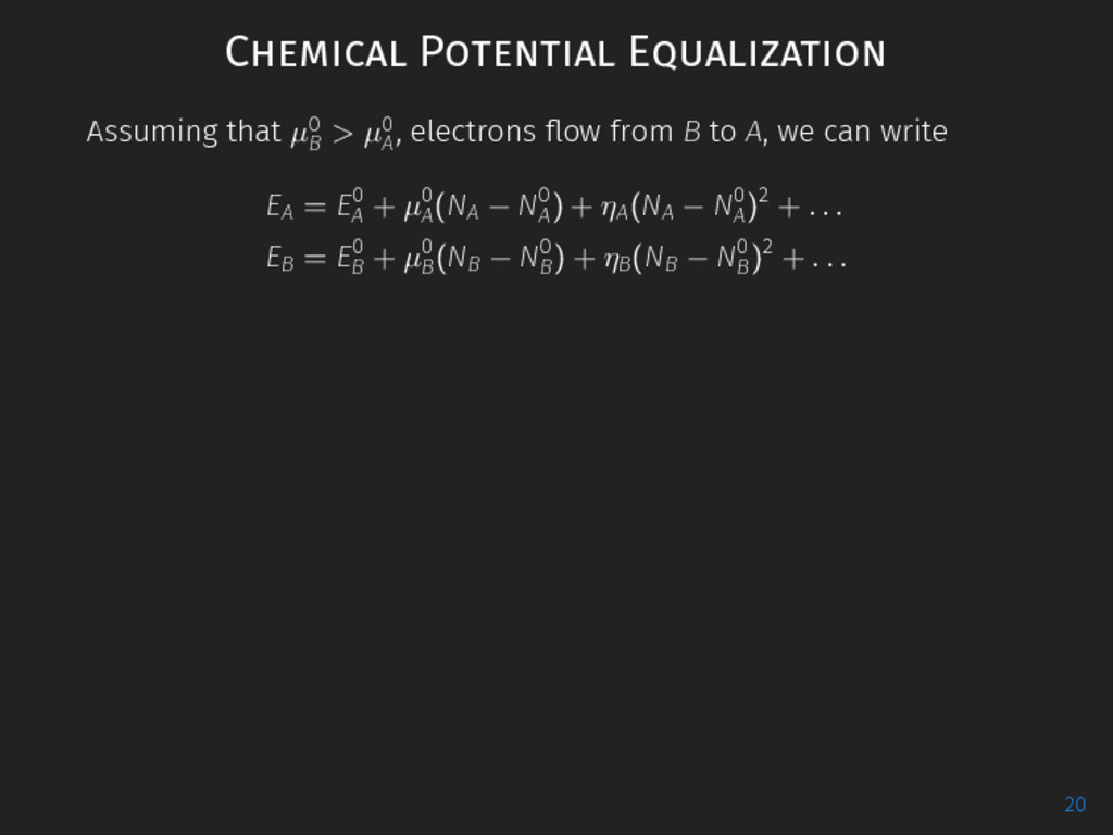
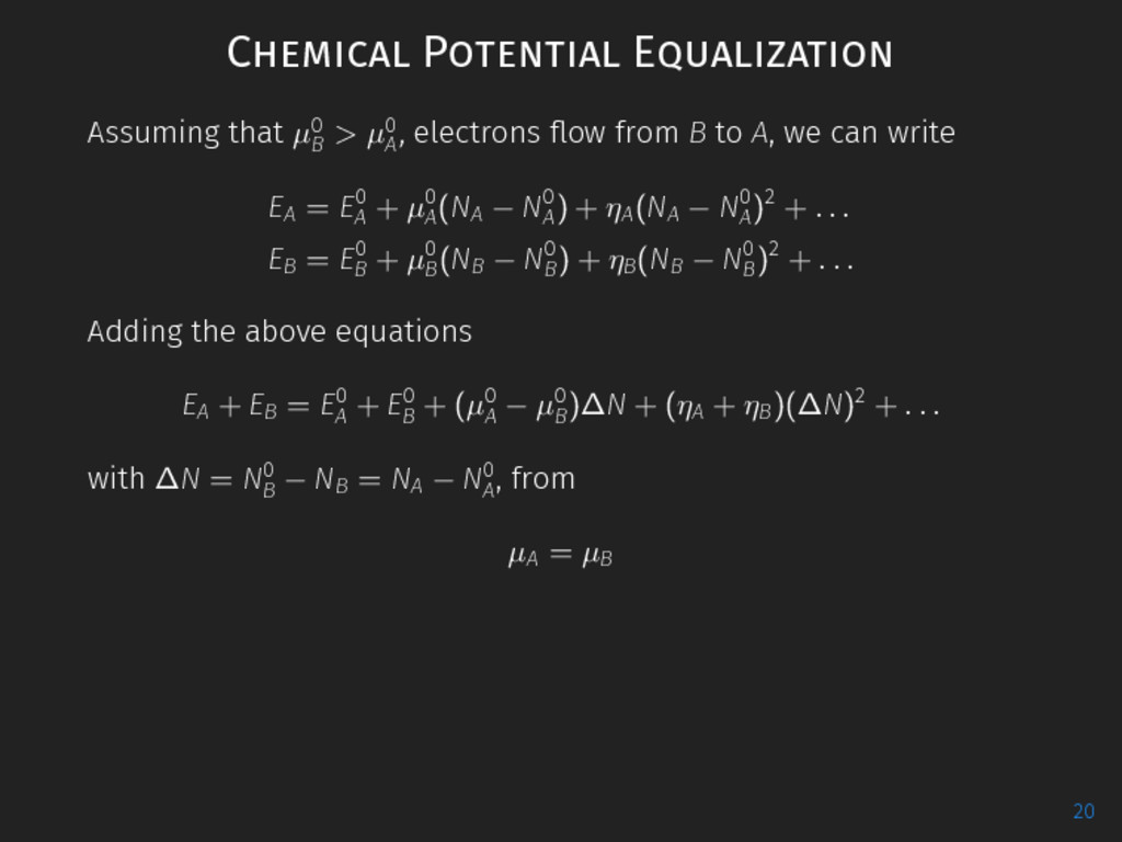
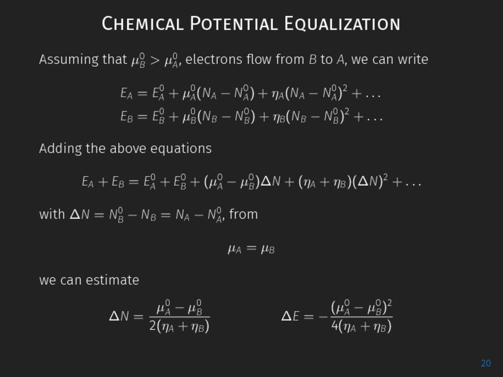
32. Chemical Potential Equalization Assuming that µ0 B > µ0 A , electrons flow from B to A, we can write EA = E0 A + µ0 A (NA − N0 A ) + ηA (NA − N0 A )2 + . . . EB = E0 B + µ0 B (NB − N0 B ) + ηB (NB − N0 B )2 + . . . 20
33. Chemical Potential Equalization Assuming that µ0 B > µ0 A , electrons flow from B to A, we can write EA = E0 A + µ0 A (NA − N0 A ) + ηA (NA − N0 A )2 + . . . EB = E0 B + µ0 B (NB − N0 B ) + ηB (NB − N0 B )2 + . . . Adding the above equations EA + EB = E0 A + E0 B + (µ0 A − µ0 B )∆N + (ηA + ηB )(∆N)2 + . . . with ∆N = N0 B − NB = NA − N0 A , from µA = µB 20
34. Chemical Potential Equalization Assuming that µ0 B > µ0 A , electrons flow from B to A, we can write EA = E0 A + µ0 A (NA − N0 A ) + ηA (NA − N0 A )2 + . . . EB = E0 B + µ0 B (NB − N0 B ) + ηB (NB − N0 B )2 + . . . Adding the above equations EA + EB = E0 A + E0 B + (µ0 A − µ0 B )∆N + (ηA + ηB )(∆N)2 + . . . with ∆N = N0 B − NB = NA − N0 A , from µA = µB we can estimate ∆N = µ0 A − µ0 B 2(ηA + ηB ) ∆E = − (µ0 A − µ0 B )2 4(ηA + ηB ) 20
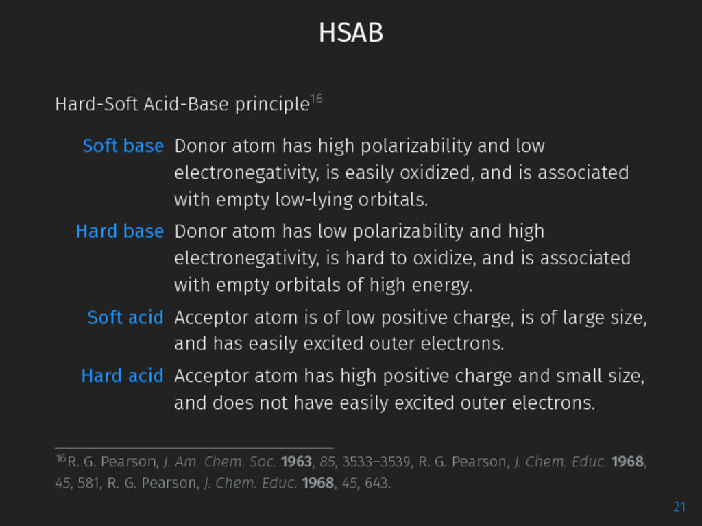
35. HSAB Hard-Soft Acid-Base principle16 Soft base Donor atom has high polarizability and low electronegativity, is easily oxidized, and is associated with empty low-lying orbitals. Hard base Donor atom has low polarizability and high electronegativity, is hard to oxidize, and is associated with empty orbitals of high energy. Soft acid Acceptor atom is of low positive charge, is of large size, and has easily excited outer electrons. Hard acid Acceptor atom has high positive charge and small size, and does not have easily excited outer electrons. 16R. G. Pearson, J. Am. Chem. Soc. 1963, 85, 3533–3539, R. G. Pearson, J. Chem. Educ. 1968, 45, 581, R. G. Pearson, J. Chem. Educ. 1968, 45, 643. 21
36. Conclusions ∙ electronegativity seems to be a versatile concept connected to various fundamental atomic properties ∙ initially developed to characterize acid-base chemistry in modern formulations still tightly linked to it ∙ easy to evaluate ∙ capable of being a powerful predictor 22
37. Questions? 23