Optimal transport on graphs with applications

Transcript

1. Optimal transport on finite graphs with applications Wuchen Li UCLA March 25, 2017
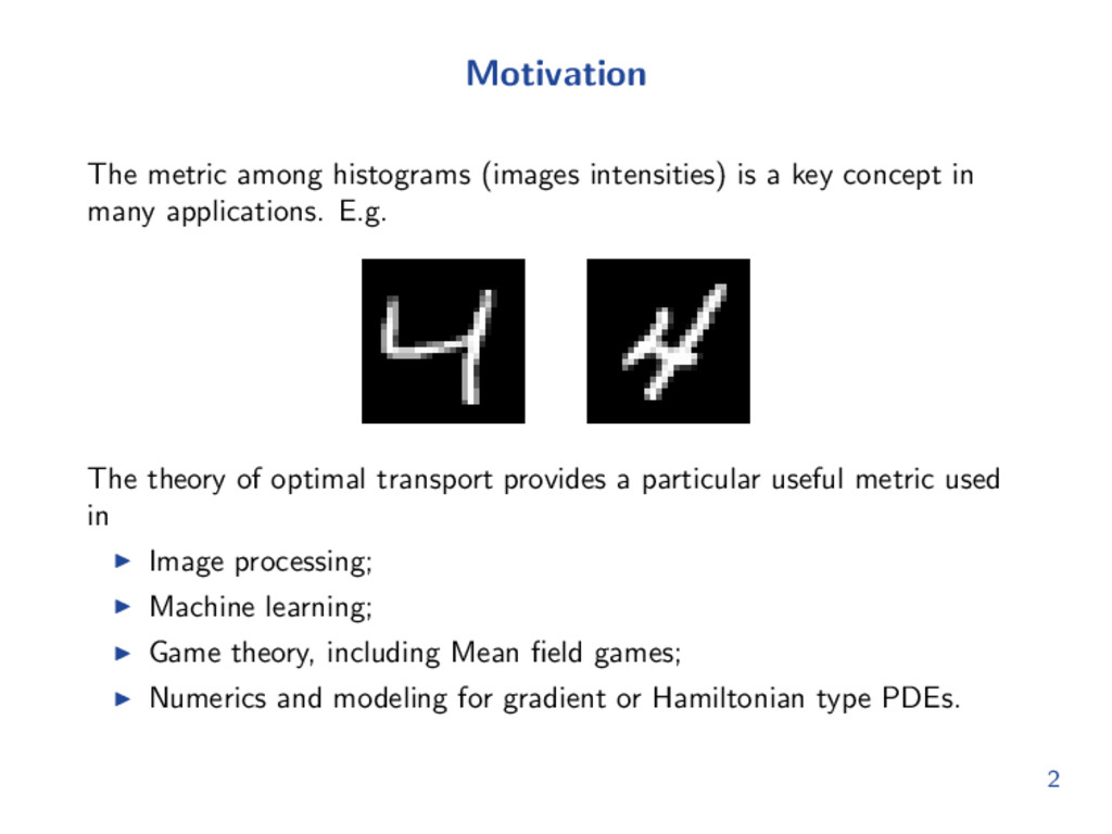
2. Motivation The metric among histograms (images intensities) is a key concept in many applications. E.g. The theory of optimal transport provides a particular useful metric used in Image processing; Machine learning; Game theory, including Mean field games; Numerics and modeling for gradient or Hamiltonian type PDEs. 2
3. Optimal transport What is the optimal way to move (transport) some dirts with shape X, density ρ0(x) to another shape Y with density ρ1(y)? The question leads to the definition of Earth Mover’s distance or Wasserstein metric. The problem is first considered by Monge in 1781, then relaxed by Kantorovich in 1940s. So it is usually named Monge-Kantorovich problem. 3
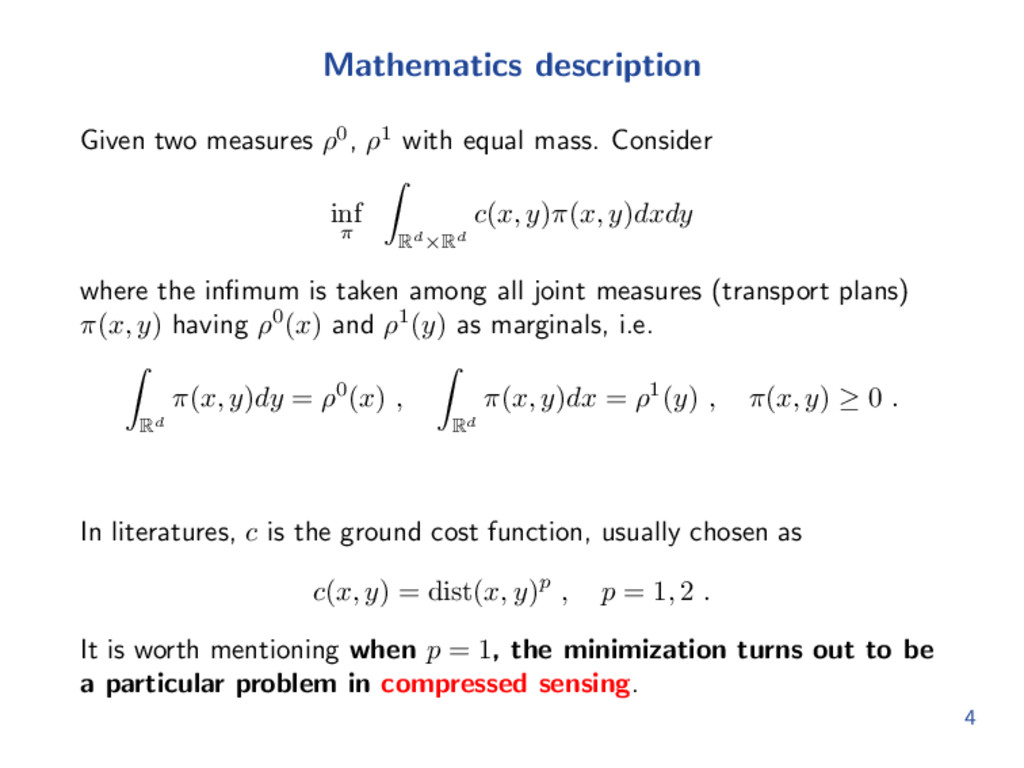
4. Mathematics description Given two measures ρ0, ρ1 with equal mass. Consider inf π Rd×Rd c(x, y)π(x, y)dxdy where the infimum is taken among all joint measures (transport plans) π(x, y) having ρ0(x) and ρ1(y) as marginals, i.e. Rd π(x, y)dy = ρ0(x) , Rd π(x, y)dx = ρ1(y) , π(x, y) ≥ 0 . In literatures, c is the ground cost function, usually chosen as c(x, y) = dist(x, y)p , p = 1, 2 . It is worth mentioning when p = 1, the minimization turns out to be a particular problem in compressed sensing. 4
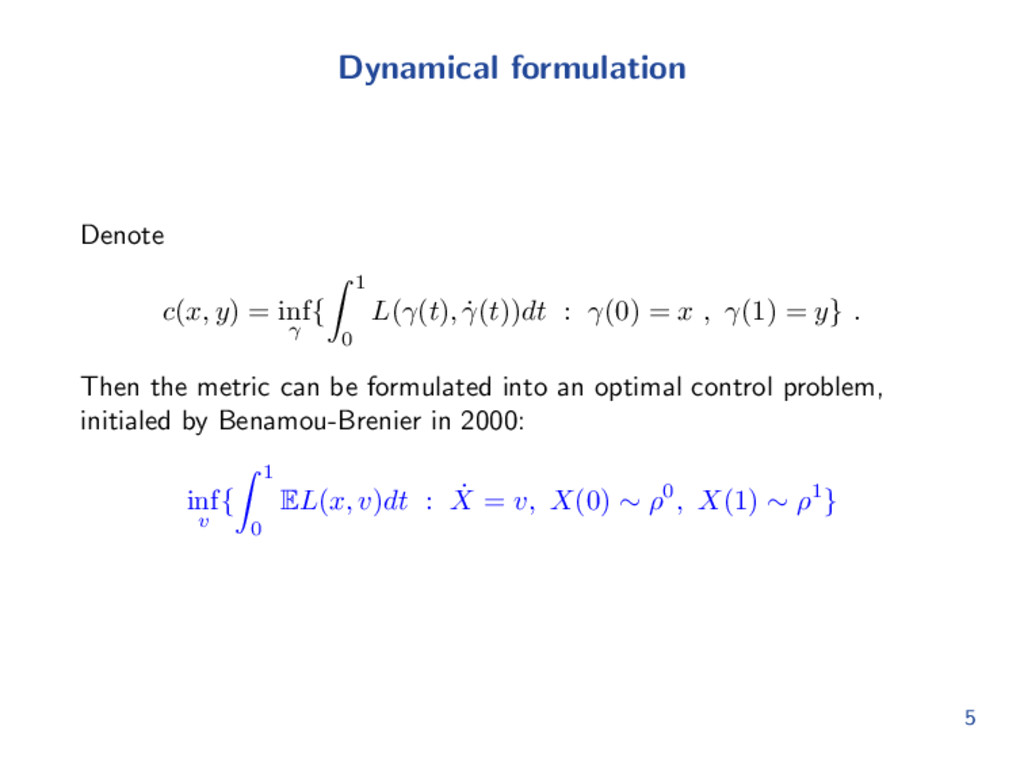
5. Dynamical formulation Denote c(x, y) = inf γ { 1 0 L(γ(t), ˙ γ(t))dt : γ(0) = x , γ(1) = y} . Then the metric can be formulated into an optimal control problem, initialed by Benamou-Brenier in 2000: inf v { 1 0 EL(x, v)dt : ˙ X = v, X(0) ∼ ρ0, X(1) ∼ ρ1} 5
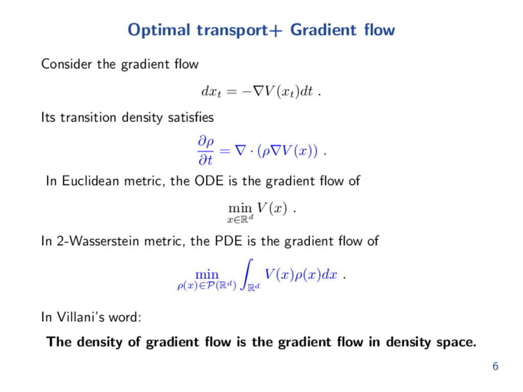
6. Optimal transport+ Gradient flow Consider the gradient flow dxt = −∇V (xt )dt . Its transition density satisfies ∂ρ ∂t = ∇ · (ρ∇V (x)) . In Euclidean metric, the ODE is the gradient flow of min x∈Rd V (x) . In 2-Wasserstein metric, the PDE is the gradient flow of min ρ(x)∈P(Rd) Rd V (x)ρ(x)dx . In Villani’s word: The density of gradient flow is the gradient flow in density space. 6
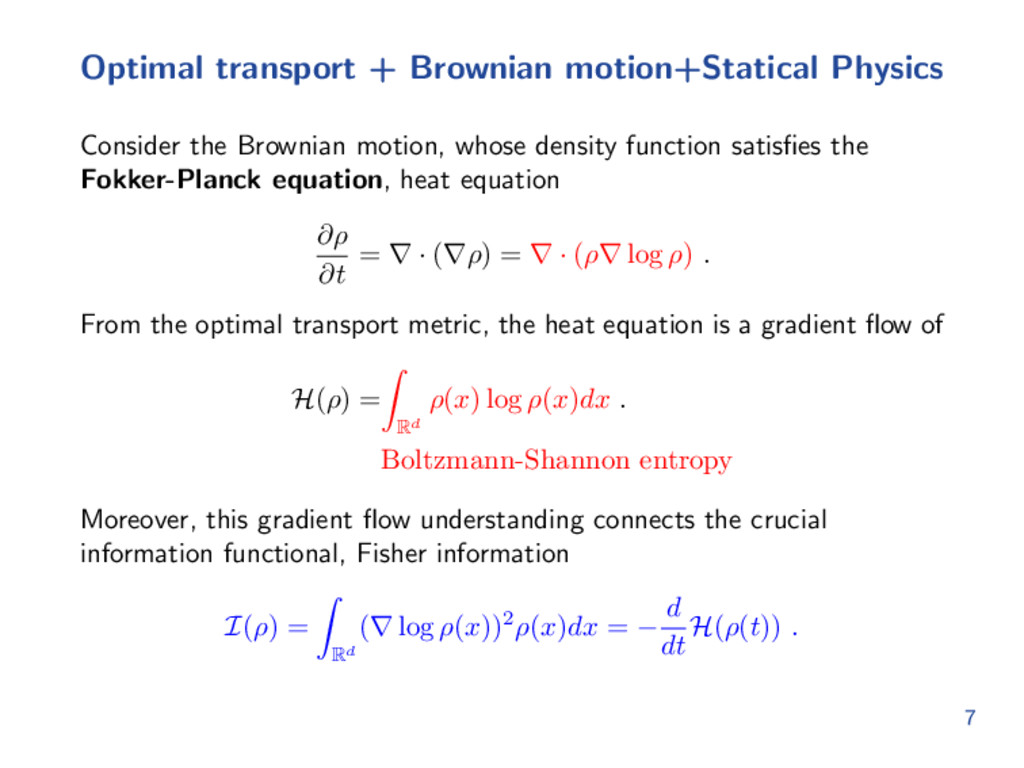
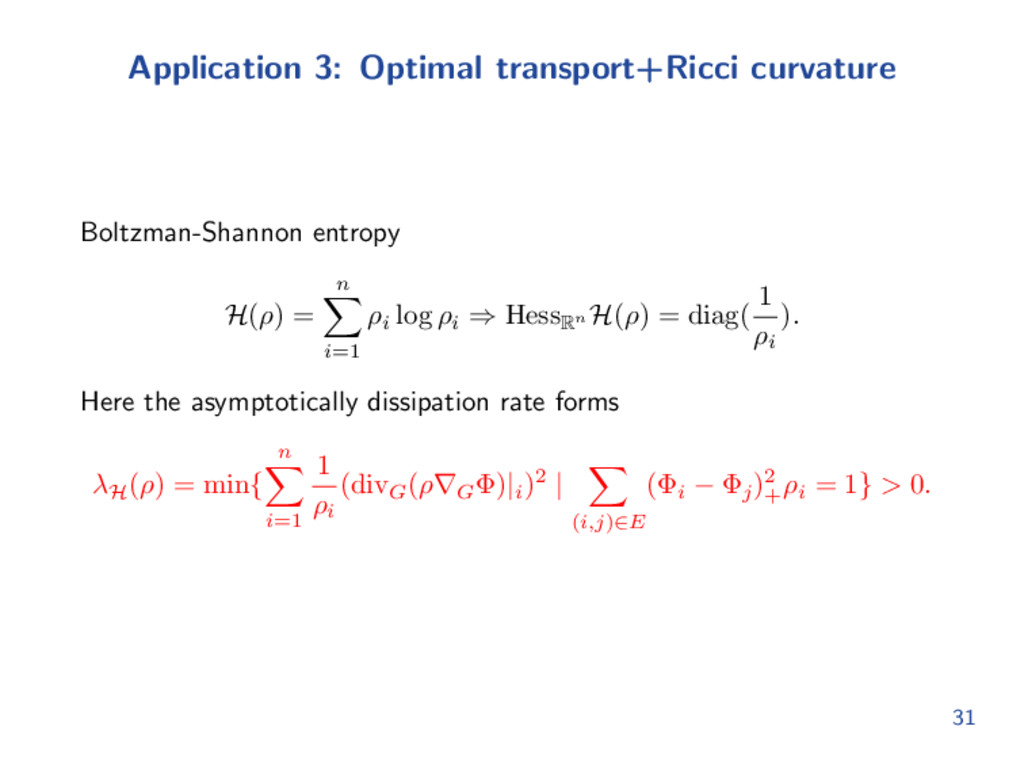
7. Optimal transport + Brownian motion+Statical Physics Consider the Brownian motion, whose density function satisfies the Fokker-Planck equation, heat equation ∂ρ ∂t = ∇ · (∇ρ) = ∇ · (ρ∇ log ρ) . From the optimal transport metric, the heat equation is a gradient flow of H(ρ) = Rd ρ(x) log ρ(x)dx . Boltzmann-Shannon entropy Moreover, this gradient flow understanding connects the crucial information functional, Fisher information I(ρ) = Rd (∇ log ρ(x))2ρ(x)dx = − d dt H(ρ(t)) . 7
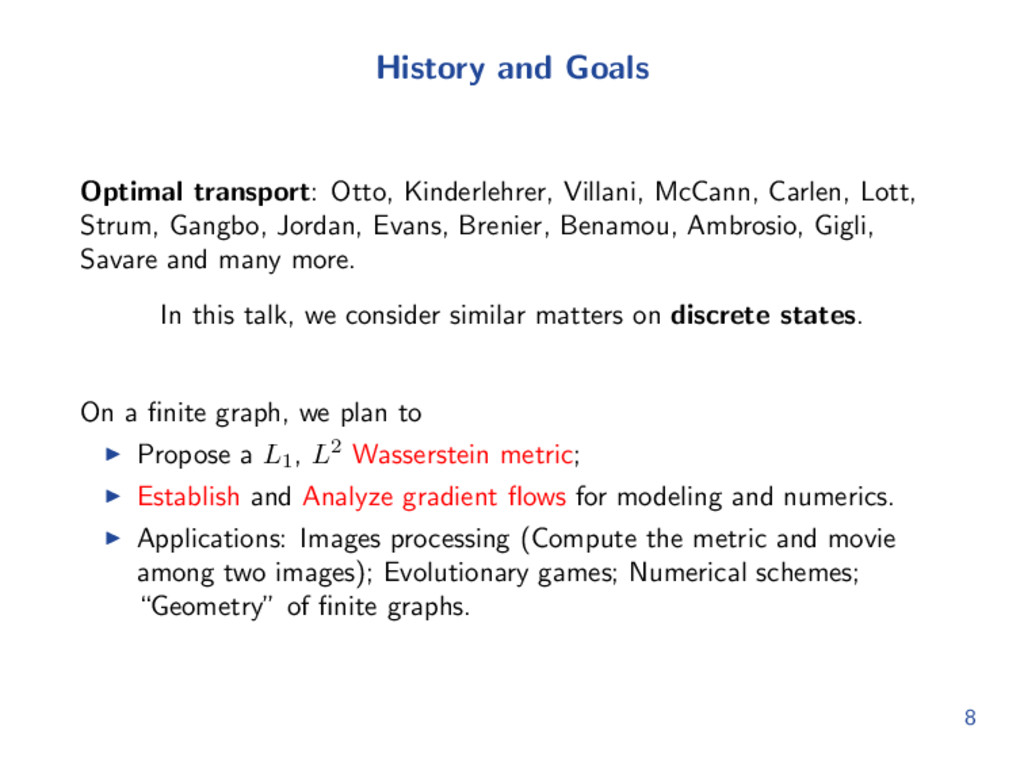
8. History and Goals Optimal transport: Otto, Kinderlehrer, Villani, McCann, Carlen, Lott, Strum, Gangbo, Jordan, Evans, Brenier, Benamou, Ambrosio, Gigli, Savare and many more. In this talk, we consider similar matters on discrete states. On a finite graph, we plan to Propose a L1 , L2 Wasserstein metric; Establish and Analyze gradient flows for modeling and numerics. Applications: Images processing (Compute the metric and movie among two images); Evolutionary games; Numerical schemes; “Geometry” of finite graphs. 8
9. Mathematical Requirements Optimizations; Optimal control and Calculus of variation; Dynamical systems; Probability; Stochastic process; Riemanian Geometry; Partial differential equations; Graph theory; Statistical Physics (Entropy + Fisher information); ... Recent Developments: Erbar, Mielke, Mass, Gigli, Strum, Villani, Olivier, Fathi, Chow, Zhou, Li, Osher and many more. 9
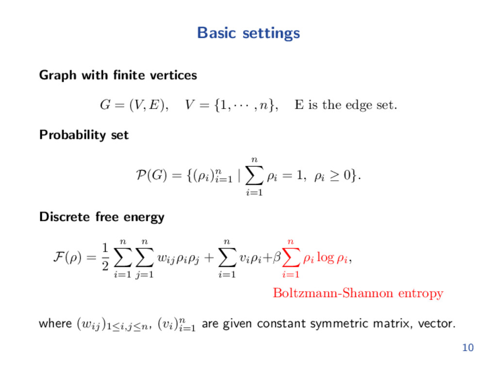
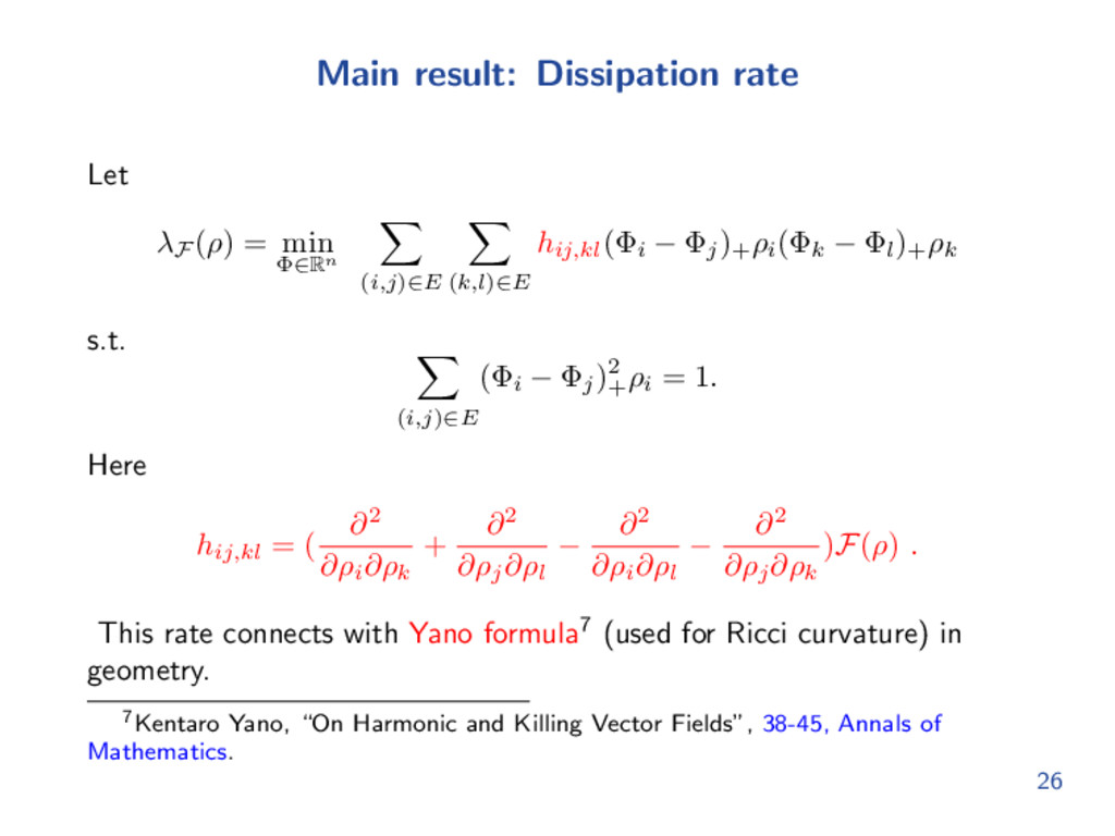
10. Basic settings Graph with finite vertices G = (V, E), V = {1, · · · , n}, E is the edge set. Probability set P(G) = {(ρi )n i=1 | n i=1 ρi = 1, ρi ≥ 0}. Discrete free energy F(ρ) = 1 2 n i=1 n j=1 wij ρi ρj + n i=1 vi ρi +β n i=1 ρi log ρi , Boltzmann-Shannon entropy where (wij )1≤i,j≤n , (vi )n i=1 are given constant symmetric matrix, vector. 10
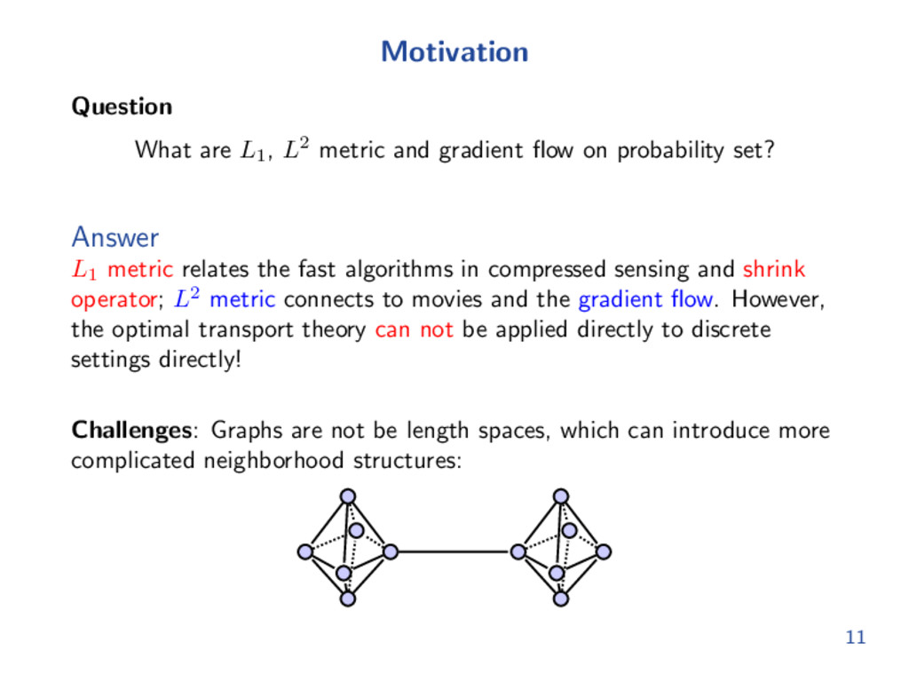
11. Motivation Question What are L1 , L2 metric and gradient flow on probability set? Answer L1 metric relates the fast algorithms in compressed sensing and shrink operator; L2 metric connects to movies and the gradient flow. However, the optimal transport theory can not be applied directly to discrete settings directly! Challenges: Graphs are not be length spaces, which can introduce more complicated neighborhood structures: 11
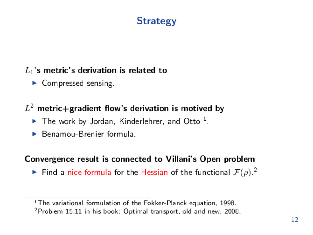
12. Strategy L1 ’s metric’s derivation is related to Compressed sensing. L2 metric+gradient flow’s derivation is motived by The work by Jordan, Kinderlehrer, and Otto 1. Benamou-Brenier formula. Convergence result is connected to Villani’s Open problem Find a nice formula for the Hessian of the functional F(ρ).2 1The variational formulation of the Fokker-Planck equation, 1998. 2Problem 15.11 in his book: Optimal transport, old and new, 2008. 12
13. Metric derivation Recall the L1 , L2-Wasserstein metric in Brenier-Benamou formula: inf v { 1 0 Rd vpρdxdt : ∂ρ ∂t + ∇ · (ρv) = 0, ρ(0) = ρ0, ρ(1) = ρ1}, where p = 1, 2. We plan to find the metric on P(G). 13
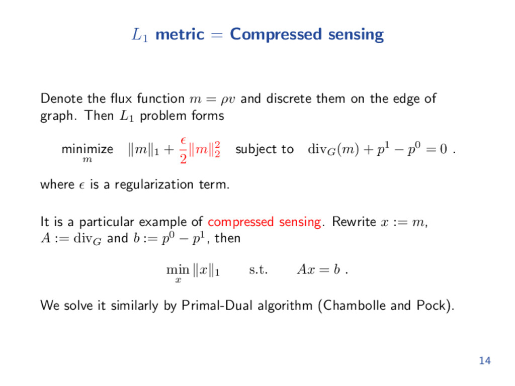
14. L1 metric = Compressed sensing Denote the flux function m = ρv and discrete them on the edge of graph. Then L1 problem forms minimize m m 1 + 2 m 2 2 subject to divG (m) + p1 − p0 = 0 . where is a regularization term. It is a particular example of compressed sensing. Rewrite x := m, A := divG and b := p0 − p1, then min x x 1 s.t. Ax = b . We solve it similarly by Primal-Dual algorithm (Chambolle and Pock). 14
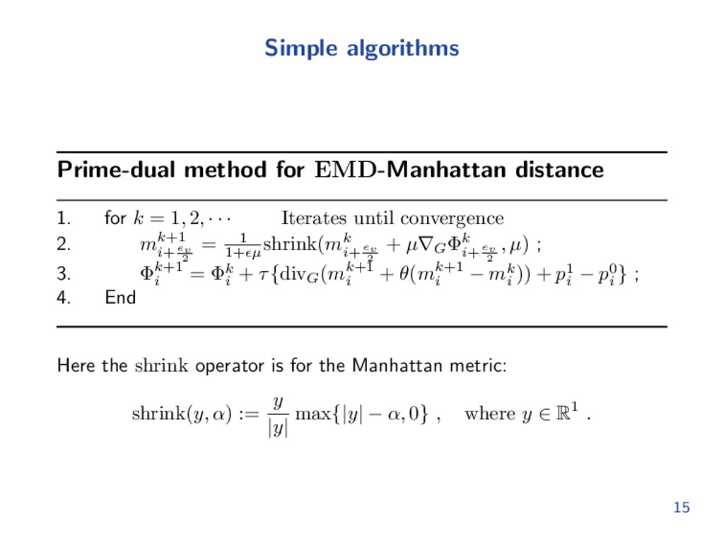
15. Simple algorithms Prime-dual method for EMD-Manhattan distance 1. for k = 1, 2, · · · Iterates until convergence 2. mk+1 i+ ev 2 = 1 1+ µ shrink(mk i+ ev 2 + µ∇G Φk i+ ev 2 , µ) ; 3. Φk+1 i = Φk i + τ{divG (mk+1 i + θ(mk+1 i − mk i )) + p1 i − p0 i } ; 4. End Here the shrink operator is for the Manhattan metric: shrink(y, α) := y |y| max{|y| − α, 0} , where y ∈ R1 . 15
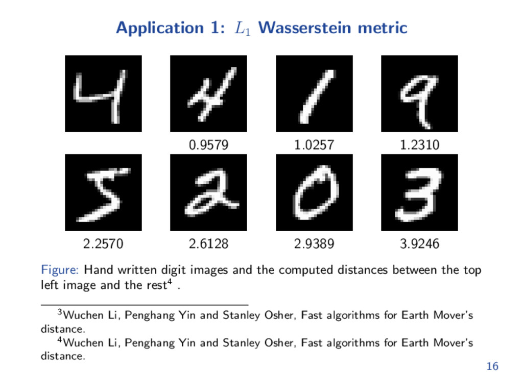
16. Application 1: L1 Wasserstein metric 0.9579 1.0257 1.2310 2.2570 2.6128 2.9389 3.9246 Figure: Hand written digit images and the computed distances between the top left image and the rest4 . 3Wuchen Li, Penghang Yin and Stanley Osher, Fast algorithms for Earth Mover’s distance. 4Wuchen Li, Penghang Yin and Stanley Osher, Fast algorithms for Earth Mover’s distance. 16
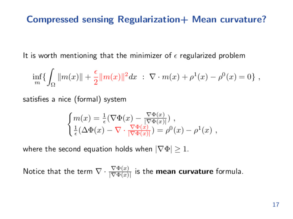
17. Compressed sensing Regularization+ Mean curvature? It is worth mentioning that the minimizer of regularized problem inf m { Ω m(x) + 2 m(x) 2dx : ∇ · m(x) + ρ1(x) − ρ0(x) = 0} , satisfies a nice (formal) system m(x) = 1 (∇Φ(x) − ∇Φ(x) |∇Φ(x)| ) , 1 (∆Φ(x) − ∇ · ∇Φ(x) |∇Φ(x)| ) = ρ0(x) − ρ1(x) , where the second equation holds when |∇Φ| ≥ 1. Notice that the term ∇ · ∇Φ(x) |∇Φ(x)| is the mean curvature formula. 17
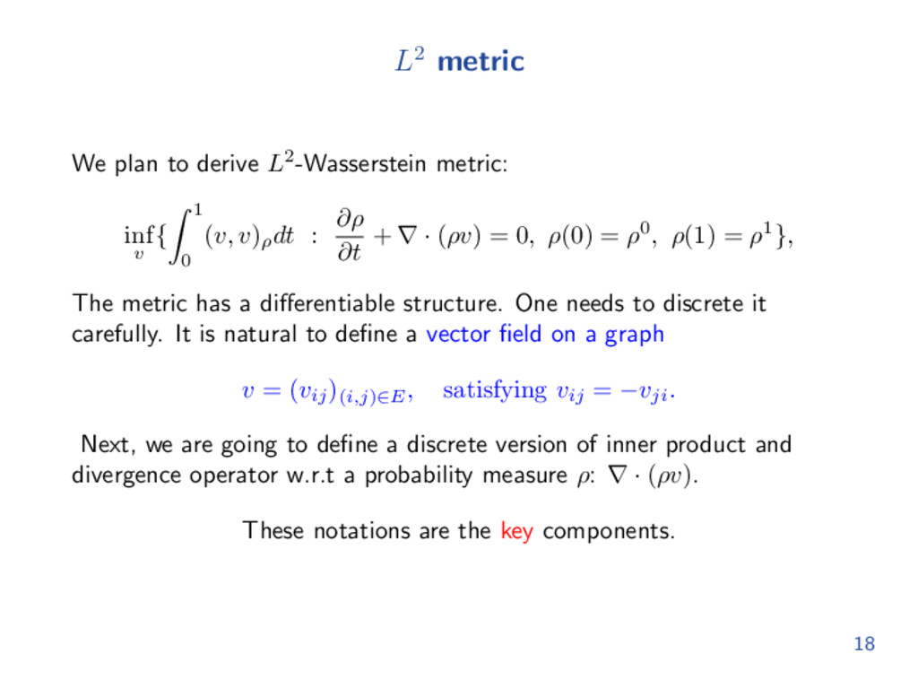
18. L2 metric We plan to derive L2-Wasserstein metric: inf v { 1 0 (v, v)ρ dt : ∂ρ ∂t + ∇ · (ρv) = 0, ρ(0) = ρ0, ρ(1) = ρ1}, The metric has a differentiable structure. One needs to discrete it carefully. It is natural to define a vector field on a graph v = (vij )(i,j)∈E , satisfying vij = −vji . Next, we are going to define a discrete version of inner product and divergence operator w.r.t a probability measure ρ: ∇ · (ρv). These notations are the key components. 18
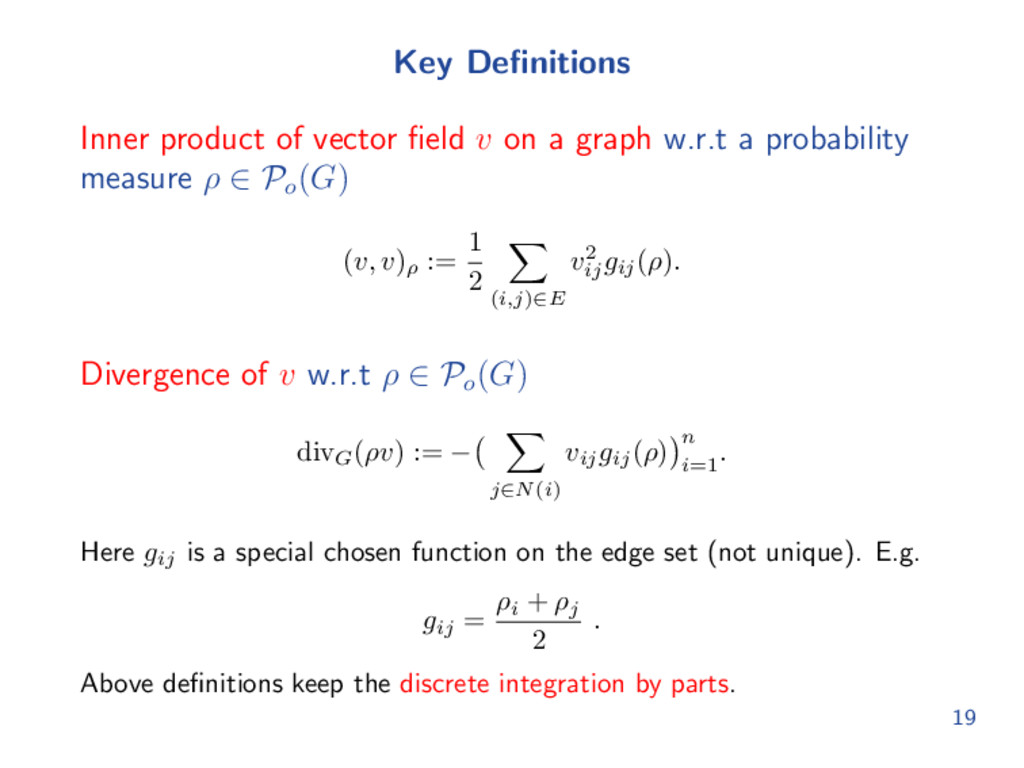
19. Key Definitions Inner product of vector field v on a graph w.r.t a probability measure ρ ∈ Po (G) (v, v)ρ := 1 2 (i,j)∈E v2 ij gij (ρ). Divergence of v w.r.t ρ ∈ Po (G) divG (ρv) := − j∈N(i) vij gij (ρ) n i=1 . Here gij is a special chosen function on the edge set (not unique). E.g. gij = ρi + ρj 2 . Above definitions keep the discrete integration by parts. 19
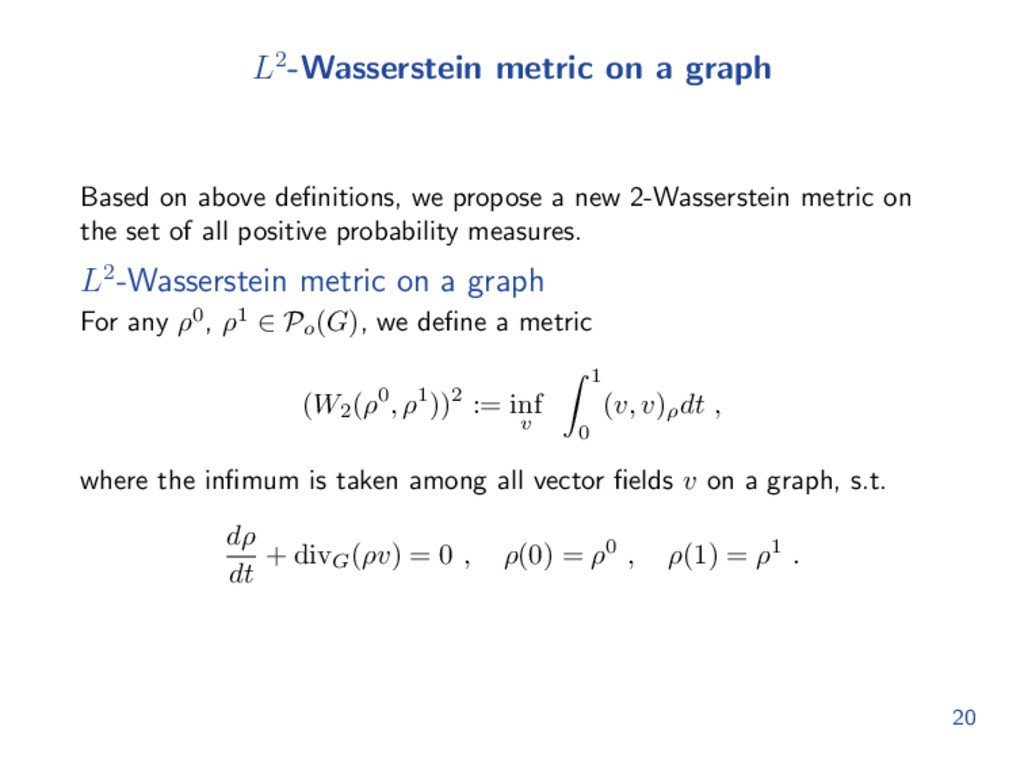
20. L2-Wasserstein metric on a graph Based on above definitions, we propose a new 2-Wasserstein metric on the set of all positive probability measures. L2-Wasserstein metric on a graph For any ρ0, ρ1 ∈ Po (G), we define a metric (W2 (ρ0, ρ1))2 := inf v 1 0 (v, v)ρ dt , where the infimum is taken among all vector fields v on a graph, s.t. dρ dt + divG (ρv) = 0 , ρ(0) = ρ0 , ρ(1) = ρ1 . 20
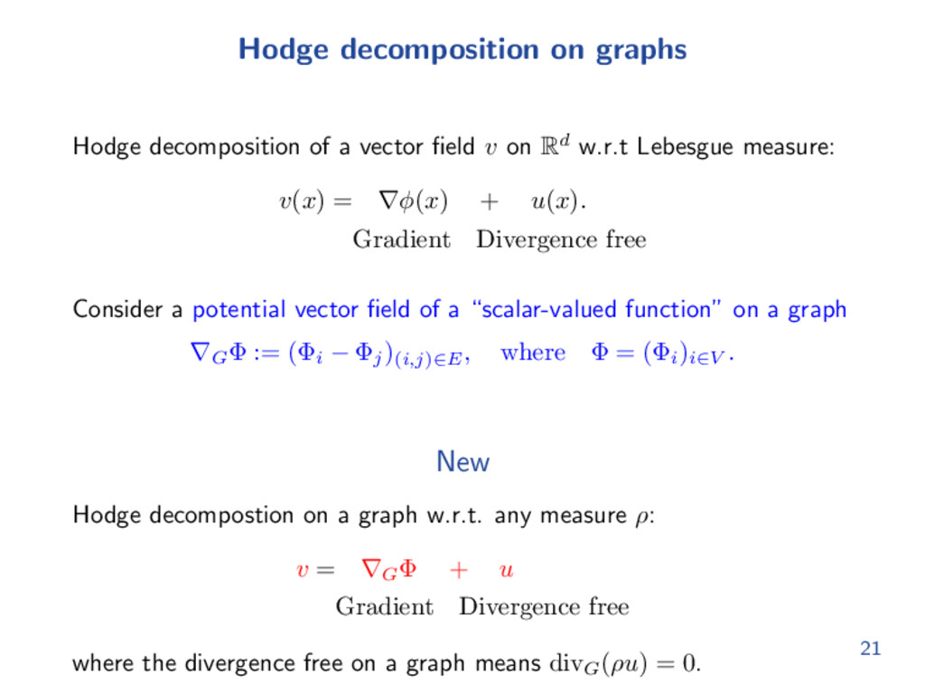
21. Hodge decomposition on graphs Hodge decomposition of a vector field v on Rd w.r.t Lebesgue measure: v(x) = ∇φ(x) + u(x). Gradient Divergence free Consider a potential vector field of a “scalar-valued function” on a graph ∇G Φ := (Φi − Φj )(i,j)∈E , where Φ = (Φi )i∈V . New Hodge decompostion on a graph w.r.t. any measure ρ: v = ∇G Φ + u Gradient Divergence free where the divergence free on a graph means divG (ρu) = 0. 21
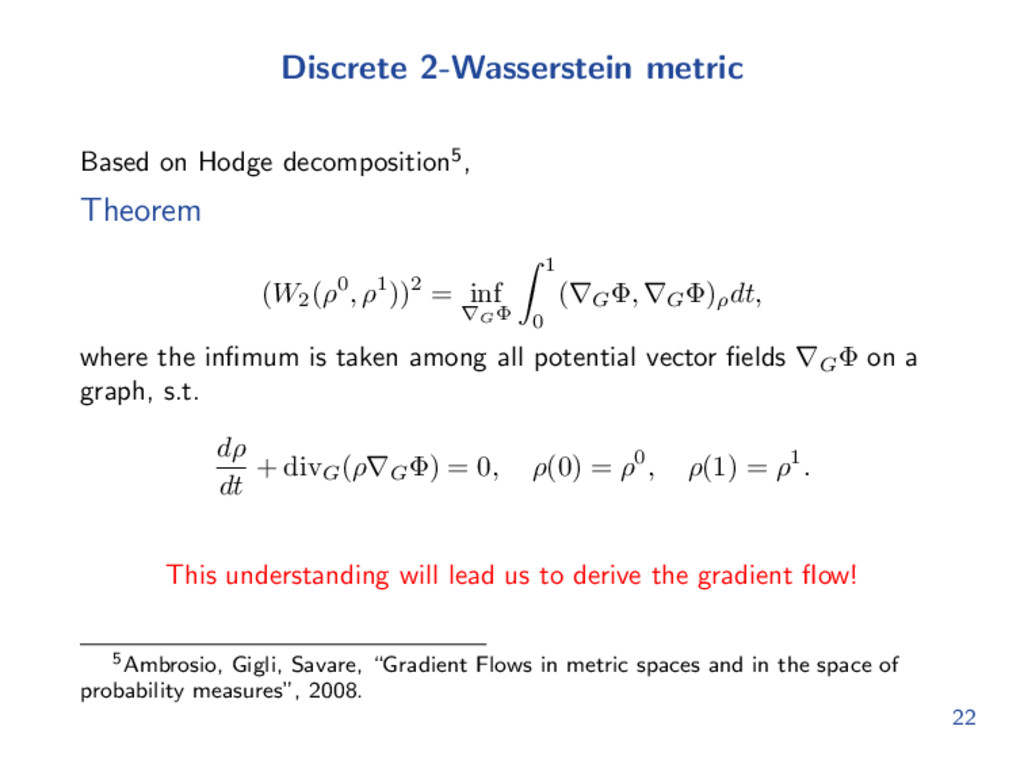
22. Discrete 2-Wasserstein metric Based on Hodge decomposition5, Theorem (W2 (ρ0, ρ1))2 = inf ∇GΦ 1 0 (∇G Φ, ∇G Φ)ρ dt, where the infimum is taken among all potential vector fields ∇G Φ on a graph, s.t. dρ dt + divG (ρ∇G Φ) = 0, ρ(0) = ρ0, ρ(1) = ρ1. This understanding will lead us to derive the gradient flow! 5Ambrosio, Gigli, Savare, “Gradient Flows in metric spaces and in the space of probability measures”, 2008. 22
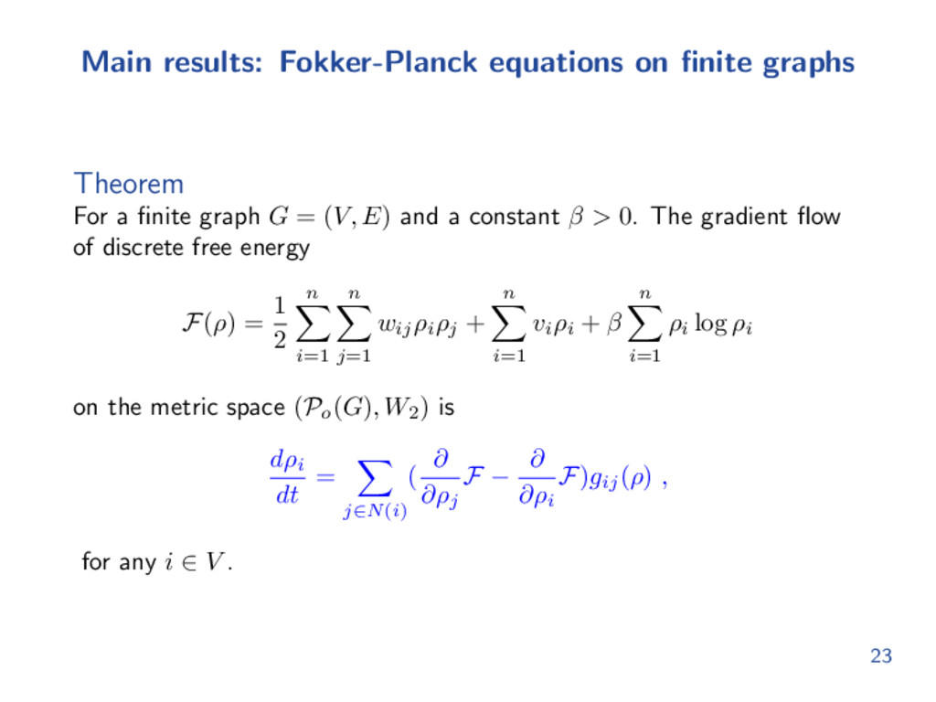
23. Main results: Fokker-Planck equations on finite graphs Theorem For a finite graph G = (V, E) and a constant β > 0. The gradient flow of discrete free energy F(ρ) = 1 2 n i=1 n j=1 wij ρi ρj + n i=1 vi ρi + β n i=1 ρi log ρi on the metric space (Po (G), W2 ) is dρi dt = j∈N(i) ( ∂ ∂ρj F − ∂ ∂ρi F)gij (ρ) , for any i ∈ V . 23
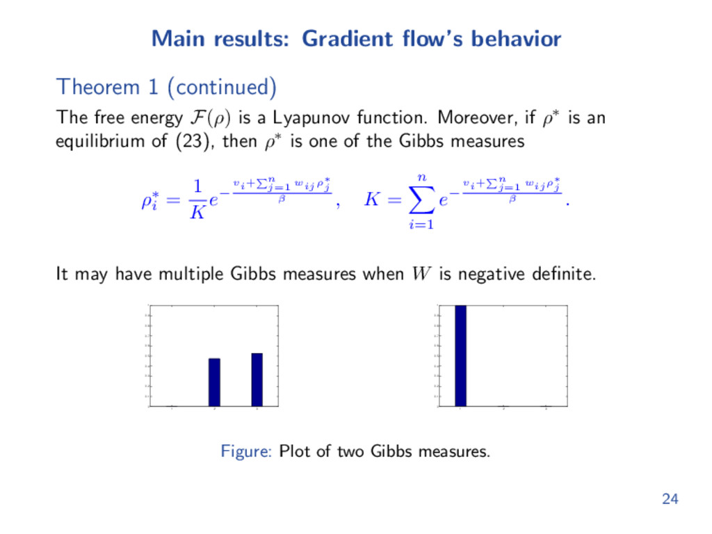
24. Main results: Gradient flow’s behavior Theorem 1 (continued) The free energy F(ρ) is a Lyapunov function. Moreover, if ρ∗ is an equilibrium of (23), then ρ∗ is one of the Gibbs measures ρ∗ i = 1 K e− vi+ n j=1 wij ρ∗ j β , K = n i=1 e− vi+ n j=1 wij ρ∗ j β . It may have multiple Gibbs measures when W is negative definite. 1 2 3 0 0.1 0.2 0.3 0.4 0.5 0.6 0.7 0.8 0.9 1 1 2 3 0 0.1 0.2 0.3 0.4 0.5 0.6 0.7 0.8 0.9 1 Figure: Plot of two Gibbs measures. 24
25. Convergence What is the rate of convergence to a Gibbs measure? Motivation Entropy dissipation: Carrillo, McCann and Villani’s work6 for nonlinear Fokker-Planck equations on Rd; Gradient flows: dynamical systems viewpoint! 6Carrillo, McCann and Villani, “Kinetic equilibration rates for granular media and related equations: entropy dissipation and mass transportation estimates”, 2003. 25
26. Main result: Dissipation rate Let λF (ρ) = min Φ∈Rn (i,j)∈E (k,l)∈E hij,kl (Φi − Φj )+ ρi (Φk − Φl )+ ρk s.t. (i,j)∈E (Φi − Φj )2 + ρi = 1. Here hij,kl = ( ∂2 ∂ρi ∂ρk + ∂2 ∂ρj ∂ρl − ∂2 ∂ρi ∂ρl − ∂2 ∂ρj ∂ρk )F(ρ) . This rate connects with Yano formula7 (used for Ricci curvature) in geometry. 7Kentaro Yano, “On Harmonic and Killing Vector Fields”, 38-45, Annals of Mathematics. 26
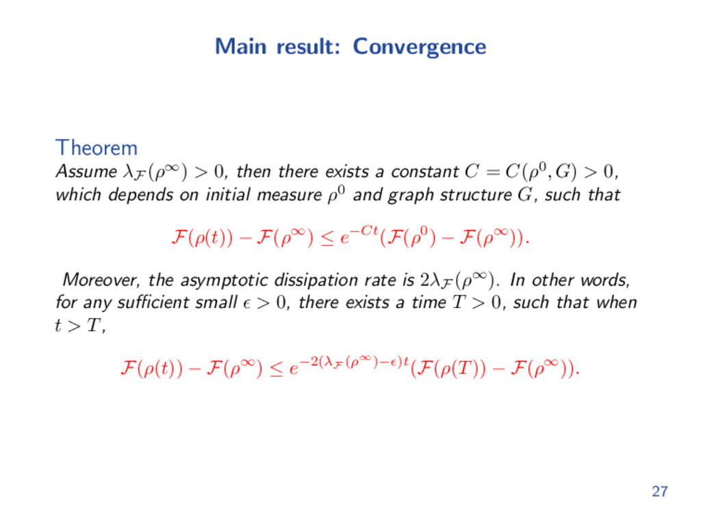
27. Main result: Convergence Theorem Assume λF (ρ∞) > 0, then there exists a constant C = C(ρ0, G) > 0, which depends on initial measure ρ0 and graph structure G, such that F(ρ(t)) − F(ρ∞) ≤ e−Ct(F(ρ0) − F(ρ∞)). Moreover, the asymptotic dissipation rate is 2λF (ρ∞). In other words, for any sufficient small > 0, there exists a time T > 0, such that when t > T, F(ρ(t)) − F(ρ∞) ≤ e−2(λF (ρ∞)− )t(F(ρ(T)) − F(ρ∞)). 27
28. Application 2: Optimal transport+ Evolutionary games Games contains8: players, strategies, payoffs. Rock-Paper-Scissors game Players: 2; Strategies: S1 = S2 = {Rock, Paper, Scissors}; Payoffs: u1 , u2 : S1 × S2 → {+1, 0, −1}. 8Wuchen Li, Phd thesis 2016. 28
29. Rock-Paper-Scissors game 1 29
30. Rock-Paper-Scissors game 2 30
31. Application 3: Optimal transport+Ricci curvature Boltzman-Shannon entropy H(ρ) = n i=1 ρi log ρi ⇒ HessRn H(ρ) = diag( 1 ρi ). Here the asymptotically dissipation rate forms λH (ρ) = min{ n i=1 1 ρi (divG (ρ∇G Φ)|i )2 | (i,j)∈E (Φi − Φj )2 + ρi = 1} > 0. 31
32. Linear Entropy+ Yano formula? Consider H(ρ) = M ρ(x) log ρ(x)dx, whose Gibbs measure is a uniform measure. Then (HessP(M) H · ∇Φ, ∇Φ)ρ∗ = M [Ric(∇Φ, ∇Φ) + D2Φ 2 HS ]ρ∗(x)dx = M [∇ · (ρ∗∇Φ)]2 1 ρ∗(x) dx. The first equality is well known derived through Bochner’s formula, while the second equality is new. This special example just shows Yano’s formula9. 9Yano: “Some Remarks on Tensor Fields and Curvature”, Annals of Mathematics, 1952. 32
33. Further Applications Applications of the L1 Earth Mover’s metric in applications, such as image processing, segmentation and color transfer; Parallel algorithms on transport related optimizations (Movies); Modeling by Fokker-Planck equations on discrete states; Mean field games (differential games); “Geometry” of graphs. 33
34. Main references Wuchen Li A study of stochastic differential equations and Fokker-Planck equations, Ph.d thesis, 2016. Wuchen Li, Stanley Osher and Wilfrid Gangbo Fast algorithm for Earth Mover’s distance, 2016. Shui-Nee Chow, Wuchen Li and Haomin Zhou Nonlinear Fokker-Planck equations on finite graphs with asymptotic properties, 2017. Shui-Nee Chow, Luca Dieci, Wuchen Li and Haomin Zhou Entropy dissipation semi-discretization schemes for Fokker-Planck equations, 2017. 34
35. Thanks! 35