Estimation of Menstrual Cycle Day using Cross-Sectional Biomarker Measurements

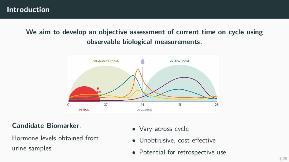
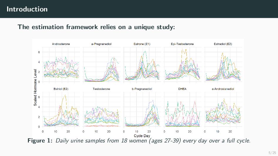
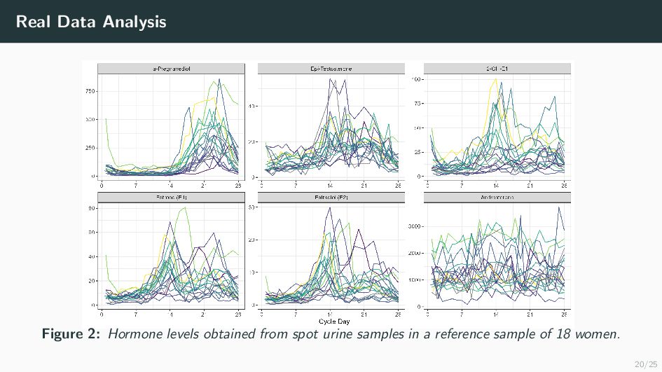
Many health-related outcomes and exposures vary over the menstrual cycle. Accounting for this source of variation could improve model accuracy and statistical power. However, cycle day is difficult to measure through self report or estimate using available methods, and is routinely overlooked in studies involving women's health. Our goal is to provide an accurate estimate of menstrual cycle day (i.e. number of days since the start of cycle) using hormone values derived from a single spot urine sample. We construct a likelihood for the latent cycle day based on observed hormone levels; this likelihood uses patterns of hormonal variation obtained from a unique study that followed a sample of women over a complete cycle as a reference. Our results suggest that we can estimate the cycle day within three days for the majority of observations based on single spot urine samples. This approach can be applied to ongoing and future studies in which menstrual cycle day is a potentially important variable, and may refine results based on extant datasets that obtained urine samples.

Transcript

1. 1/25 Estimation of Menstrual Cycle Day using Cross-Sectional Biomarker Measurements Madison Stoms, Lauren Houghton, Mary Beth Terry, Kathleene Ulanday, Julie Herbstman, & Jeff Goldsmith
2. 2/25 Motivation Many outcomes/exposures vary across the menstrual cycle i.e. weight, breast tissue density, cognition, and energy levels. Many of these changes are mediated by varying hormone levels.
3. 3/25 Motivation Failing to account for cycle day negatively impacts the ability to accurately model outcomes and detect other effects.
4. 4/25 Introduction We aim to develop an objective assessment of current time on cycle using observable biological measurements. Candidate Biomarker: Hormone levels obtained from urine samples • Vary across cycle • Unobtrusive, cost effective • Potential for retrospective use
5. 5/25 Introduction The estimation framework relies on a unique study: Figure 1: Daily urine samples from 18 women (ages 27-39) every day over a full cycle.
6. 6/25 Methods: Univariate Setting Scenario: We observe a single scalar value ynew from a continuous process ynew (t) on t ∈ [0, 28] without knowledge of the true observation time θ. Assumptions: We know the true population parameters which describe the data generating mechanism of ynew (t) Goal: Construct a likelihood to estimate θ
7. 7/25 Methods: Univariate Setting KL Expansion for Observed Hormone Level at θ: ynew = ynew (θ) = µ(θ) + K k=1 ξnew,k ϕk(θ) + ϵnew ξnew ∼ N(0, Λ), ϵnew ∼ N(0, σ2 ϵ ) Known: {µ, Φ, Λ, σ2 ϵ , K} Unknown: {θ, ξnew }
8. 8/25 Methods: Univariate Setting Sample from a Known Data Generating Mechanism
9. 9/25 Methods: Univariate Setting Observed Value
10. 10/25 Methods: Univariate Setting To construct the likelihood, we evaluate the probability of a certain ˜ θ generating ynew and iterate across all possible points.
11. 11/25 Methods: Univariate Setting Likelihood Construction: At a particular ˜ θ we construct an estimate for ynew (t) and consider the following questions, Piece 1: How likely is the estimated hormone trajectory given the assumed data generating mechanism? Piece 2: How large is the residual between the estimated trajectory and observed value?
12. 12/25 Methods: Univariate Setting Estimated hormone trajectory for ynew at θ
13. 13/25 Methods: Univariate Setting Estimated Hormone Trajectory for ynew at θ: Piece 1: likelihood of the trajectory given the data generating mechanism Piece 2: Residual between the trajectory and ynew
14. 14/25 Methods: Univariate Setting Likelihood at θ:
15. 15/25 Methods: Multivariate Setting If we observe levels for multiple hormones across a cycle, we can incorporate this information into our likelihood. ynew = (y(1) new , ..., y(L) new ) from latent time θ We use multivariate FPCA to account for score correlation and construct a multivariate likelihood (Happ & Greven, 2018).
16. 16/25 Methods: Multivariate Setting Observed Values at True Observation Point
17. 17/25 Methods: Multivariate Setting Univariate Likelihoods
18. 18/25 Methods: Multivariate Setting Multivariate Likelihood
19. 19/25 Methods: Estimation In practice {µ, Φ, Λ, σ2 ϵ , K} are unknown. We estimate them using a reference sample observed across known time points. yi (tij ) = µ(tij ) + K k=1 ξikϕk(tij ) + ϵij ti = (ti1, ...., tiJi ) can be dense or sparse at the subject level.
20. 20/25 Real Data Analysis Figure 2: Hormone levels obtained from spot urine samples in a reference sample of 18 women.
21. 21/25 Real Data Analysis Analysis Procedure (LOOCV) 1. Choose a test subject 2. Sample a random time point, θ, and take corresponding hormone level as ynew 3. Estimate parameters using training data 4. Approximate θ and evaluate dist(ˆ θ, θ) Perform 15 repetitions of steps 2 - 4 for each subject
22. 22/25 Real Data Analysis Figure 3: Error distributions across various hormone sets and thresholds.
23. 23/25 Discussion Summary We are able to obtain an accurate estimate of cycle day which can be used to account for sources of variability attributed to the menstrual cycle. The use of spot urine samples makes this method highly accessible and opens the potential for retrospective use.
24. 24/25 Discussion Limitations • Small, unrepresentative sample • Lack of understanding in regards to hormonal variation across and within women Future Directions • Test performance on richer data set • Accounting for uncertainty in time estimates
25. 25/25 Discussion Thank you for listening! Questions? Contact: Madison Stoms (ms5975@cumc.columbia.edu)