Linear Regression Basics

Transcript

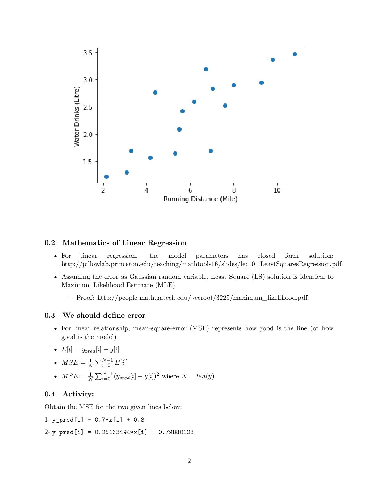
1. Linear_Regression_Book July 23, 2021 0.1 Linear Regression • We want to present the relationship between variables (features and target) linearly • For simplicity, consider we have one feature denoted as the running distance and target variable know as drinking water • We are interested to obtain the best line describing by y_pred[i] = w_1 x[i] +w_0 that map running distance (x[i]) to drinking water estimation (y_pred[i]) while we know, y[i], the true values for drinking water • Then, when we only know the running distance, the model can predict the amount of water that the runner would drink [3]: import numpy as np import matplotlib.pyplot as plt # Running Distance in Mile x = np.array([3.3,4.4,5.5,6.71,6.93,4.168,9.779,6.182,7.59,2.167, 7.042,10.791,5.313,7.997,5.654,9.27,3.1]) # Water Drinks in Litre y = np.array([1.7,2.76,2.09,3.19,1.694,1.573,3.366,2.596,2.53,1.221, 2.827,3.465,1.65,2.904,2.42,2.94,1.3]) plt.scatter(x, y) plt.xlabel('Running Distance (Mile)') plt.ylabel('Water Drinks (Litre)') [3]: Text(0, 0.5, 'Water Drinks (Litre)') 1
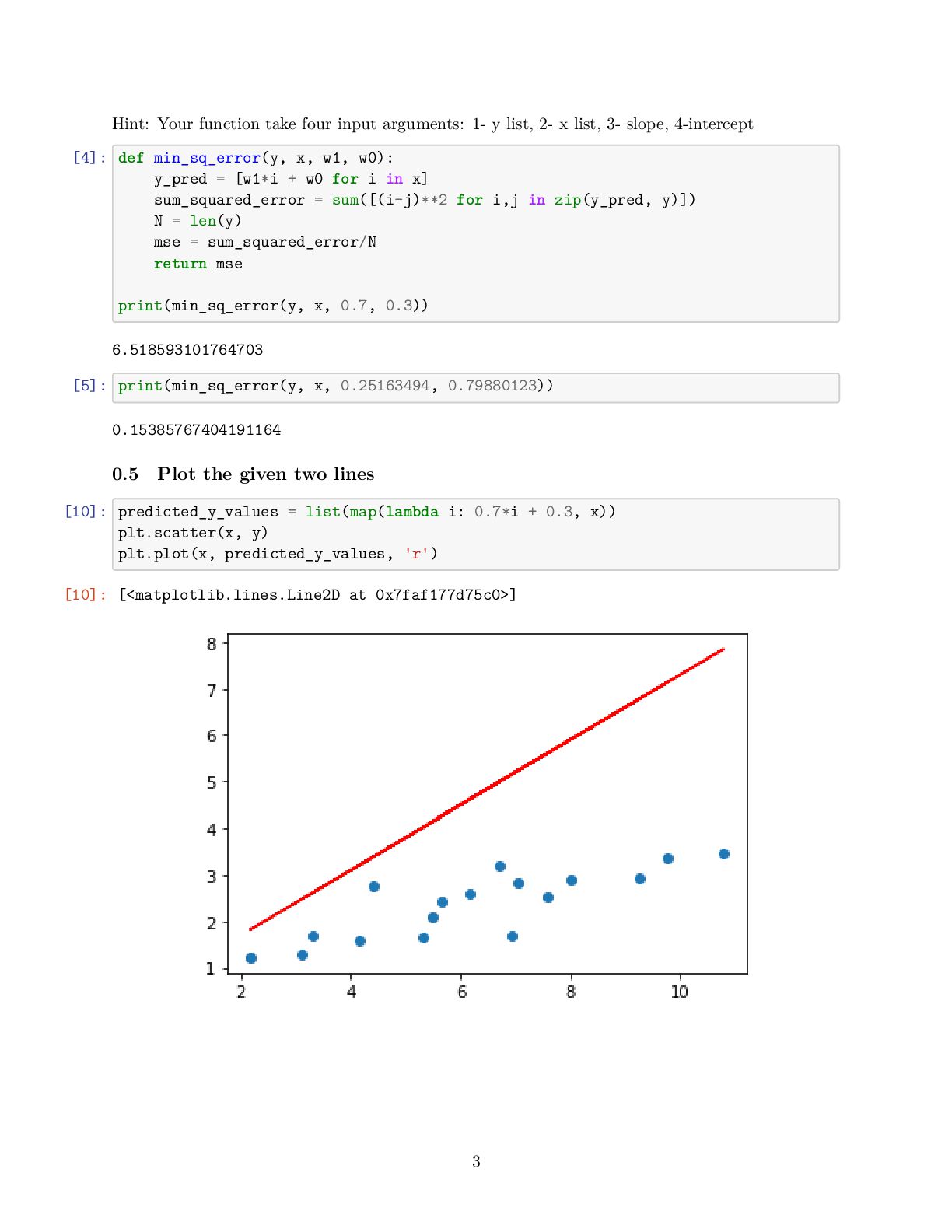
2. 0.2 Mathematics of Linear Regression • For linear regression, the model parameters has closed form solution: http://pillowlab.princeton.edu/teaching/mathtools16/slides/lec10_LeastSquaresRegression.pdf • Assuming the error as Gaussian random variable, Least Square (LS) solution is identical to Maximum Likelihood Estimate (MLE) – Proof: http://people.math.gatech.edu/~ecroot/3225/maximum_likelihood.pdf 0.3 We should define error • For linear relationship, mean-square-error (MSE) represents how good is the line (or how good is the model) • E[i] = ypred[i] − y[i] • MSE = 1 N ∑ N−1 i=0 E[i]2 • MSE = 1 N ∑ N−1 i=0 (ypred[i] − y[i])2 where N = len(y) 0.4 Activity: Obtain the MSE for the two given lines below: 1- y_pred[i] = 0.7*x[i] + 0.3 2- y_pred[i] = 0.25163494*x[i] + 0.79880123 2
3. Hint: Your function take four input arguments: 1- y list, 2- x list, 3- slope, 4-intercept [4]: def min_sq_error(y, x, w1, w0): y_pred = [w1*i + w0 for i in x] sum_squared_error = sum([(i-j)**2 for i,j in zip(y_pred, y)]) N = len(y) mse = sum_squared_error/N return mse print(min_sq_error(y, x, 0.7, 0.3)) 6.518593101764703 [5]: print(min_sq_error(y, x, 0.25163494, 0.79880123)) 0.15385767404191164 0.5 Plot the given two lines [10]: predicted_y_values = list(map(lambda i: 0.7*i + 0.3, x)) plt.scatter(x, y) plt.plot(x, predicted_y_values, 'r') [10]: [<matplotlib.lines.Line2D at 0x7faf177d75c0>] 3
4. [11]: predicted_y_values = list(map(lambda i: 0.25163494*i + 0.79880123, x)) plt.scatter(x, y) plt.plot(x, predicted_y_values, 'r') [11]: [<matplotlib.lines.Line2D at 0x7faf17420438>] 0.6 Mathematically: MSE = 1 N ∑ N−1 i=0 (ypred[i] − y[i])2 which is equal to MSE = 1 N ∑ N−1 i=0 (w1x[i] + w0 − y[i])2 Compute: ∂MSE ∂w1 and ∂MSE ∂w0 then obtain w1 and w0 such that : ∂MSE ∂w1 = 0 and ∂MSE ∂w0 = 0 ∂MSE ∂w1 = 2 N ∑ N−1 i=0 x[i](w1x[i] + w0 − y[i]) = 2 N w1 ∑ N−1 i=0 x[i]2 + 2 N w0 ∑ N−1 i=0 x[i] − 2 N ∑ N−1 i=0 x[i]y[i] = 2w1x2 + 2w0x − 2xy ∂MSE ∂w0 = 2 N ∑ N−1 i=0 (w1x[i] + w0 − y[i]) = 2w1x + 2w0 − 2y 4
5. 0.7 Activities: [3]: from scipy import stats slope, intercept, r_value, p_value, std_err = stats.linregress(x, y) [16]: print(slope) 0.25163494428355404 5
6. [17]: print(intercept) 0.7988012261753894 [18]: print("r-squared:", r_value**2) r-squared: 0.6928760302783604 [4]: print(std_err) 0.0432568020417479 0.8 Write a function that returns MSE and Error list [17]: def min_sq_error(y, x, w1, w0): y_pred = [w1*i + w0 for i in x] error = [(i-j) for i,j in zip(y_pred, y)] sum_squared_error = sum([(i-j)**2 for i,j in zip(y_pred, y)]) N = len(y) mse = sum_squared_error/N return mse, error print(min_sq_error(y, x, 0.25163494, 0.79880123)[1]) [-0.07080346800000004, -0.8540050339999998, 0.09279340000000014, -0.7027283226000001, 0.8486313642000001, 0.27461565992000003, -0.10646069174000017, -0.24159157091999983, 0.17871042459999975, 0.12309414497999982, -0.25618552252000004, 0.0491938675400001, 0.4857376662199999, -0.09287415482000005, -0.1984548192400002, 0.1914571237999998, 0.27886954399999997] 0.9 Obtain the mean and std of error for optimal line [18]: np.mean(min_sq_error(y, x, 0.25163494, 0.79880123)[1]) np.std(min_sq_error(y, x, 0.25163494, 0.79880123)[1]) [18]: 0.39224695542720417 0.10 Plot the distribution of the error list for optimal line [20]: import seaborn as sns sns.distplot(min_sq_error(y, x, 0.25163494, 0.79880123)[1], hist=True,␣ → kde=True, bins=4) /Users/miladtoutounchian/anaconda3/lib/python3.6/site- packages/seaborn/distributions.py:2557: FutureWarning: `distplot` is a deprecated function and will be removed in a future version. Please adapt your code to use either `displot` (a figure-level function with similar flexibility) 6
7. or `histplot` (an axes-level function for histograms). warnings.warn(msg, FutureWarning) [20]: <AxesSubplot:ylabel='Density'> 0.11 Write your own function that computes R Squared [34]: def f_r_sq(y, x, w1, w0): y_pred = [w1*i + w0 for i in x] SS_res = sum([(i-j)**2 for i,j in zip(y_pred, y)]) SS_tot = sum([(i - np.mean(y))**2 for i in y]) return 1- SS_res/SS_tot print(f_r_sq(y, x, 0.25163494, 0.79880123)) 0.692876030278359 0.12 Derive the slope and intercept • After taking partial derivative of mean-squared-error and setting to zero for both w1 and w0 (∂MSE ∂w1 = 0 ∂MSE ∂w0 = 0) • w1 = xy−¯ x¯ y x2−x2 • w0 = y − w1x 7
8. [50]: def slope_intercept_LR(x, y): w1 = (np.mean([i*j for i, j in zip(x, y)]) - np.mean(x)*np.mean(y))/(np. → mean([i*i for i in x]) - np.mean(x)**2) w0= np.mean(y) - w1*np.mean(x) return w1, w0 print(slope_intercept_LR(x, y)) (0.25163494428355315, 0.7988012261753947) 0.13 In almost all applications we update the slope and intercept through iter- ation • w1 = w1 − η ∗ ∂MSE ∂w1 • w0 = w0 − η ∗ ∂MSE ∂w0 [5]: xx_bar = np.mean([i*i for i in x]) xy_bar = np.mean([i*j for i, j in zip(x, y)]) x_bar = np.mean(x) y_bar = np.mean(y) w_0 = np.random.randn() w_1 = np.random.randn() print(w_1) print(w_0) epoch = 5000 for _ in range(epoch): w_1 = w_1 - 0.01*(2*w_1*xx_bar + 2*w_0*x_bar-2*xy_bar) w_0 = w_0 - 0.01*(2*w_1*x_bar+2*w_0-2*y_bar) print(w_1) print(w_0) -0.6054090863116374 0.08001160212963707 0.2516353668855077 0.7987982302621295 1 Optional reading: • It is better to have while loop, if | J(w(n+1) 1 , w(n+1) 0 ) − J(w(n) 1 , w(n) 0 ) |≤ ϵ stop the while loop • n represents the nth-iteration [1]: # It is better to have while loop, if |J(w1,w0) at n+1 iteration - J(w1,w0) at␣ → n iteration|<=eps stop the while loop import numpy as np # Running Distance in Mile 8
9. x = np.array([3.3,4.4,5.5,6.71,6.93,4.168,9.779,6.182,7.59,2.167, 7.042,10.791,5.313,7.997,5.654,9.27,3.1]) # Water Drinks in Litre y = np.array([1.7,2.76,2.09,3.19,1.694,1.573,3.366,2.596,2.53,1.221, 2.827,3.465,1.65,2.904,2.42,2.94,1.3]) N = len(y) xx_bar = np.mean([i*i for i in x]) xy_bar = np.mean([i*j for i, j in zip(x, y)]) x_bar = np.mean(x) y_bar = np.mean(y) w_0 = np.random.randn() w_1 = np.random.randn() iteration = 0 while True if iteration == 0 else np.abs(E2 - E1) >= 0.000000001: y_pred = [w_1*i + w_0 for i in x] error = [(i-j) for i,j in zip(y_pred, y)] sum_squared_error = sum([(i-j)**2 for i,j in zip(y_pred, y)]) E1 = sum_squared_error/N w_1 = w_1 - 0.01*(2*w_1*xx_bar + 2*w_0*x_bar-2*xy_bar) w_0 = w_0 - 0.01*(2*w_1*x_bar+2*w_0-2*y_bar) y_pred = [w_1*i + w_0 for i in x] error = [(i-j) for i,j in zip(y_pred, y)] sum_squared_error = sum([(i-j)**2 for i,j in zip(y_pred, y)]) E2 = sum_squared_error/N iteration += 1 print(w_1) print(w_0) print(iteration) 0.25181483605486216 0.7975259359450246 2430 1.1 Use sklearn to obtain the best line [4]: from sklearn.linear_model import LinearRegression lr_reg = LinearRegression() lr_reg.fit(x.reshape(-1, 1), y) 9
10. print(lr_reg.coef_) print(lr_reg.intercept_) [0.25163494] 0.7988012261753894 10